A Classification Framework for Large-Scale Face
Recognition Systems
Ziheng Zhou, Samuel Chindaro and Farzin Deravi Department of Electronics, University of Kent
Canterbury, UK CT2 7NT {z.zhou, s.chindaro and f.deravi}@kent.ac.uk
Abstract. This paper presents a generic classification framework for large-scale face recognition systems. Within the framework, a data sampling strategy is proposed to tackle the data imbalance when image pairs are sampled from thousands of face images for preparing a training dataset. A modified kernel Fisher discriminant classifier is proposed to make it computationally feasible to train the kernel-based classification method using tens of thousands of training samples. The framework is tested in an open-set face recognition scenario and the performance of the proposed classifier is compared with alternative techniques. The experimental results show that the classification framework can effectively manage large amounts of training data, without regard to feature types, to efficiently train classifiers with high recognition accuracy compared to alternative techniques.
Keywords: classification framework, face recognition and kernel Fisher discriminant.
1 Introduction
In the past two decades, there has been a great deal of research and development in the field of face recognition (FR) [14]. To develop a large-scale practical FR system, it is essential to use a large facial image database for training and testing so that real-world scenarios that may be faced in target applications can be effectively represented. Fortunately, some large databases have been built up for testing various FR technologies [8-10].
It is well known that the task of face recognition can be turned into a simple and effective two-class classification problem [4,6,7]. To do that, facial features are extracted from an image pair (instead of a single image) and then classified into the intra- and extra-personal categories. Here, the intra-personal features represent those calculated from two images of the same persons while the extra-personal features are calculated from two images from different persons.
Although adopting the classification problem is not new in the literature, using it to build up an FR system based on a large facial database (e.g., the Face Recognition Grand Challenge (FRGC) database [9]) still remains challenging. The first major challenge is how to handle the large amount of training data. For example, if the FRGC database is used and only the controlled frontal images are exploited,
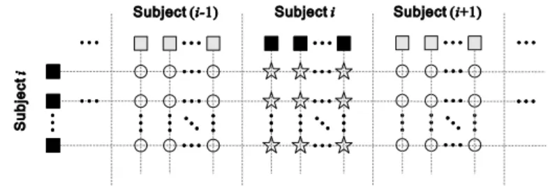
according to [9], there are more than 20 thousand such images from which more than 400 million image pairs can be sampled for training and testing. Moreover, the number of intra-personal image pairs and extra-personal image pairs are extremely imbalanced. Fig. 1 shows an example that explains such imbalance. In the figure, the black squares represent images of Subject and rest of the squares stand for other images in the database. The stars mark all possible intra-personal image pairs that can be sampled for Subject , while the circles locate the extra-personal image pairs. It is obvious that in a large database, there will be much more extra-personal image pairs than the intra-personal pairs for every Subject , resulting in the huge imbalance. Here, the question turns to be how to sample image pairs to form a balanced training dataset with a reasonable size.
The way that the training and test data are defined depends on whether a FR application is a close-set or an open-set problem. For an open-set problem, the system will be expecting in the test data some subjects which have not been encountered at the training phase. For a close-set scenario, all subjects in the test are also included in the training set. In recent evaluation campaigns [10], it has been observed that the open-set scenario could show a much lower FR performance compared to a closed-set scenario. Very often, a real-world large-scale FR system is required to deal with an open-set scenario. Therefore, the second challenge will be how to properly select and train a classifier using the available training data to classify the test data from some unknown subjects.
In this paper, we propose a generic classification framework to tackle the above-mentioned challenges. The framework consists of an image-pair sampling strategy for preparing a balanced set of samples for training and a kernel-based classifier that can perform reasonably in an open-set scenario and can be trained using a large training dataset. The framework is essentially “feature agnostic” – meaning that it is independent of the choice feature-extraction algorithms used to produce training and test vectors for classification. The multi-resolution local binary pattern (LBP) [1] features are used to test the system on the FRGC database. Experiments are designed to simulate the open-set scenario and results indicate that the framework significantly improves the performance.
The rest of the paper is organised as follows: Section 2 and 3 describes the sampling strategy and the classifier, respectively. The experiments and results are presented in Section 4. Section 5 provides a summary and conclusions.
Fig. 1. An example showing the imbalance between the number of intra-personal image pairs and the number of extra-personal image pairs that can be sampled for Subject . The black squares represent images of Subject and rest of the squares stand for other images in the
database. The stars mark all possible intra-personal image pairs that can be sampled for Subject , while the circles locate the extra-personal image pairs.
2 Data Sampling Strategy
As mentioned above, a large facial database (e.g., the FRGC database) could contain thousands of face images from which millions of image pairs can be sampled for training and test purposes. The huge amount of data available and the imbalance between the numbers of intra- and extra-personal image pairs make the preparation of a suitable training dataset non-trivial for any FR system.
To cope with the large number of training samples and to make each subject evenly weighted in the training dataset, one common way [13] is to select equal number of images for each subject and sample all the intra- and extra-personal image pairs from the selected images. By evenly weighted, we mean that the numbers of intra- and extra-personal image pairs including images of a particular subject should be the same for each subject. Although the method is intuitively straightforward, the obtained training dataset is not suitable for the classification problem as explained in the example below.
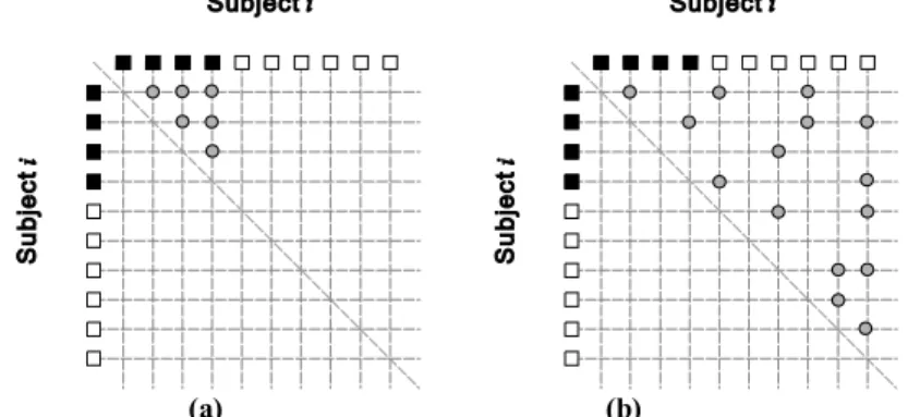
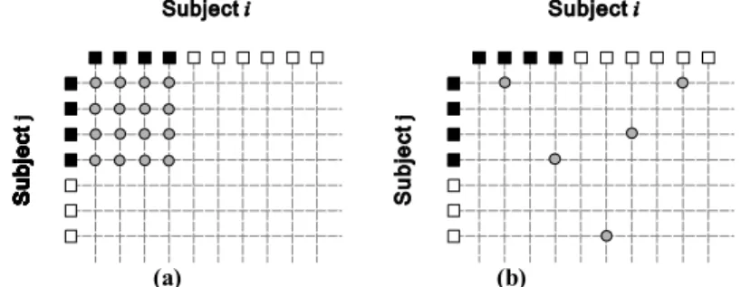
Suppose that there is a database containing = 300 subjects (a large facial database could include many more subjects) and for each subject, = 4 images are randomly selected. Assume that there are ten images from Subject and seven images from Subject . Fig. 2(a) and Fig. 3(a) show the intra-personal pairs sampled for Subject and extra-personal pairs sampled for Subject and . (Note that without loss of generality, images belonging to a subject can always be organised in the order that starts with the selected images represented by the black boxes.) Here the image pair ( , ) is considered to be the same as ( , ) and the pairs formed by the same images are only included once. The total number of intra-personal pairs can be calculated as ( − 1) = 1800 and the total number of extra-personal pairs can be calculated as ( − 1) which is more than 7 × 10 . The disadvantage of the sampling method is that and are decided by given and ≪ always holds no matter how changes. Besides the large imbalance between and , from the figures, it can been that the image pairs are not randomly sampled from all the possible positions.
In this paper, we propose a strategy for sampling a balanced dataset in which each subject is evenly weighted. Here the subjects involved in the sampling are denoted as , , … , and the images from as , , … , where is the number of images. Instead of selecting images for each subject, we first list all the intra- and extra-personal pairs. For , the intra-personal pairs can be expressed as:
In Eq. (1), the image index is always smaller than to avoid including an image pair twice and to exclude those formed by the same images. For a subject pair , ( < ), the extra-personal pairs can be expressed as:
,
= , |1 ≤ ≤ , 1 ≤ ≤ . (2)
In Eq. (2), the subject index is always smaller than to avoid considering a subject pair twice. We then randomly choose pairs from each and pairs from each , to form the training dataset. In this way, the total numbers of the intra- and extra-personal pairs can be computed as:
= =1
2 ( − 1) (3)
It can be seen that given fixed , and are controlled by and , respectively. The number / can be customised to enlarge/limit the number of intra-/extra-personal image pairs in the training dataset. Following the sampling example mentioned above, Fig. 2(b) and 3(b) show the image pairs obtained using the proposed sampling strategy where = 15 and =5. It can be seen that not only twice more intra-personal pairs are selected, but more images of Subject are involved in the sampled image pairs, which in some sense makes the image pairs more representative for Subject . On the other hand, because of = 5, the number of extra-personal pairs is significantly reduced to one third of the previous size. Note that subjects in a large database often have more images and a larger can be chosen to sample more intra-personal pairs.
(a) (b)
Fig. 2. The intra-personal image pairs sampled for Subject using (a) the normal image-based sampling method and (b) the proposed image-pair-based sampling strategy.
(a) (b)
Fig. 3. The extra-personal image pairs sampled for Subject and Subject using (a) the normal image-based sampling method and (b) the proposed image-pair-based sampling strategy.
3 Modified Kernel Fisher Discriminant
For an effective FR system, the choice of the classifier is equally important as the selection of informative and discriminatory features, especially for an open-set problem. In some cases, a simple classifier (e.g., a K-nearest neighbour classifier or a Bayesian classifier [6]) can do the job. However, if sufficient training data is available, a more sophisticated classifier could significant improve the system performance particularly when the extracted features have a complex distribution in the feature space. Recently, the kernel-based classification methods (e.g., the support vector machine (SVM) [11] and the kernel Fisher discriminant (KFD) [5]) have been widely used to solve some non-linear classification problems [4,5,7,13]. If two classes of data points cannot be separated sufficiently in the original space, the kernel methods provide a way to map the points into a higher-dimensional feature space in which they could distribute more sparsely and therefore, more easily be separated. The merit of these methods is that the computation of the mapping can be avoided by the ‘kernel trick’ [11] which makes it computationally feasible and affordable.
Let Φ be the mapping to the new feature space ℱ and Φ( ) ∈ ℱ be the point mapped from a data sample . The kernel is a function defined in the original space to calculate the dot product of two mapped samples Φ( )and Φ( ′), that is, ( , ′) = 〈Φ( ),Φ( ′)〉. In both SVM and KFD, the gram matrix [11] is calculated from all the training samples to solve some optimisation problem. Each entry ( , ) is defined as the value of the kernel , where and are the and samples in the training dataset. According to the definition, the dimension of matrix will be × where is the total number of samplesfor training. Although a sampling strategy has been proposed to significantly reduce the size of the training data, as there are possibly hundreds of subjects included in the database, there could still be tens of thousands of image pairs selected for training according to Eq. (3), which would make very large. Keeping such a large matrix not only requires a large amount of memory, but makes the optimisation problem computationally very expensive, sometimes even infeasible. To solve the problem, Joachims [3] developed the SVM system, an implementation of an SVM learner which addresses the problem of having large training dataset. In this paper, a modified KFD (MKFD) is proposed to tackle the problem in a more efficient way.
Let { , … , } be the training samples. The classic KFD algorithm tries to search a vector ∗∈ ℱ that maximises the ratio of the intra-class variations of the mapped feature points over the extra-class variations. Using the theory of reproducing kernels [11], can be written as a linear combination of all the samples, that is, = ∑ Φ( ). Using the kernel trick, the problem can be converted to find the optimal parameters ∗that maximises ℐ( ) = TT where = [ , , … , ] .The definitions of matrices and can be found in [5]. In this case, and can be easily computed from and to keep both matrices makes the computation more difficult.
A similar situation is encountered in the SVM where a set of parameters is to be optimised. It is known that only depends on a subset of training samples (the support vectors). The support vectors are found by solving an optimisation problem which itself involves the calculation of and only those parameters corresponding to the support vectors have non-zero values. Inspired by the finding from the SVM, we modify the KFD algorithm by selecting a subset of the training samples (obtained by the sampling strategy) to construct the linear combination for . The samples in are half intra-personal and half extra-personal and are randomly selected from the training dataset. Let = { } be the indices of the selected samples. Zero values are assigned to all the where is not in . In this way, only
, , … , need to be optimised, which makes the KFD computationally feasible for a large training dataset. Although not using the full set of the training samples might cause some information loss, the experimental results show that significant improvement can still be achieved by the MKFD method when compared with alternative techniques.
4 Experiments and Results
4.1 Experimental Setting
Experiments have been designed to test the system in a face verification scenario. A subset of the FRGC database was used. In total, the subset contains 16 thousands face images all taken under a controlled environment (e.g., with a static clear background and controlled lighting) during the 2003-2004 academic year. The large size of the set of images makes it suitable for demonstrating the proposed framework. The normalisation procedure described in [2] was used to pre-process images in the experiments.
Results can be influenced by the choice of particular training and test data. To reduce this effect, we prepared seven image groups each of which contained images from 50 subjects. In total, there were 12992 face images in the groups. Note that the subjects in each group were unique and did not appear in the other groups thereby simulating an open-set scenario very often encountered in a practical large-scale FR system. Cross validation was adopted to test the system, using one image group for validating and the rest of the images for training. The validating set was changed from one group to another until all the groups had been used.
Since the proposed classification framework does not specify any feature extraction method, the local binary pattern (LBP) technique described in [1] was used to extract facial features for testing the framework. To have different kinds of facial features, images were partitioned into 3 × 4, 5 × 5, 7 × 7, 10 × 10 and 14 × 14 local regions and three different LBP operators LBP, , LBP, and LBP , (see [1] for
details) were exploited, resulting in totally 15 kinds of facial features. For an image pair, the chi-square distances were computed from the local LBP histograms as the facial features. Note that all the features were zero-score normalised [12] in the experiments.
To prepare the training datasets, we need to decide the values of n and n . Some experiments were carried out using training datasets with different sizes and based on the results we set = 100 and = 5. For the test datasets, all the intra- and extra-personal image pairs were used to calculate the test samples. To employ MKFD, two most commonly used kernels were tested: the RBF kernels, , ′ = exp(−‖ − ′‖/ ) and the polynomial kernels, , ′ =
( ∙ ′) where and are positive constants. The RBF kernels largely outperformed the polynomial kernels and were used in the experiments. Finally, the size of the subset in the MKFD was chosen to be 5000 based on some exploratory experiment.
4.2 Experimental Results
In the first experiment, following [1], face images were partitioned into 7 × 7 local regions and the LBP features were extracted using LBP, . The classification
framework was performed on the seven image groups defined for the cross-validation. To test the robustness of the framework, in each turn of the cross-validation, we sampled three different training datasets using the sampling strategy. The MKFD classifier was then trained on them and tested on the same test dataset. To compared with the framework, we implemented the LBP system developed in [1], the linear Fisher discriminant (LFD) classifier, and the SVM [3]. Here the LFD and the SVM are trained on the same training datasets as used by the MKFD classifier.
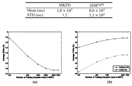
Table 1 and Fig. 4 show the results in terms of the equal error rates (EERs) and the true acceptance rates (TARs) at the false acceptance rates (FARs) of 0.1% and 1% which are two important rates for evaluating system performance [7,9]. Based on the same facial features, the proposed classification framework and the SVM system significantly outperform the other two methods. Considering the EERs, the proposed framework performed slightly better than the SVM system. Table 2 summarises the CPU time used to train the MKFD classifier and the SVM system. (Experiments were carried out on a PC with an Intel Core 2 Duo 2.4Hz CPU and 4G memory.) It can be seen that using the same training datasets, the SVM required eight times more training time than the MKFD. Moreover, there were averagely 9.57 × 10 support vectors learned by the SVM system each time, while the size of the subset used by the MKFD was set to be 5000 all the time.
In the second experiment, we investigated how the size of the subset could affect the performance of the MKFD. Using the same training and test datasets in the first experiment, different sizes of were chosen to train and test the MKFD.
Fig. 4. Average TARs reported at the FARs of 0.1% and 1%.
Table 1. Means and STDs of the EERs for different algorithms tested in the first experiment.
LBP System LFD MKFD SVM
Mean (%) 6.10 4.98 3.52 3.87
STD (%) 1.43 1.33 1.11 1.23
Table 2. Means and STDs of the CPU time used to train the MKFD and SVM .
MKFD SVM
Mean (sec) 1.0 × 10 8.0 × 10 STD (sec) 1.2 1.1 × 10
(a) (b) Fig. 5. Different sizes of the subset are chosen to train and test the MKFD classifier. The average EERs and TARs at the FARs of 0.1% and 1% are reported in (a) and (b), respectively.
Fig. 5(a) shows the EERs at the different sizes of . The rates dropped quickly from the size of 100 to 2500. After that, the curve reached the bottom at the size of 5000. It can be seen that although the size of was increased by half from 5000 to 7500, the EER remained almost unchanged, which indicates that increasing the size of does not always help to increase the performance. Fig. 5(b) shows the corresponding average TARs at the FARs of 0.1% and 1%. Once again, the two curves confirmed the finding in Fig. 5(a).
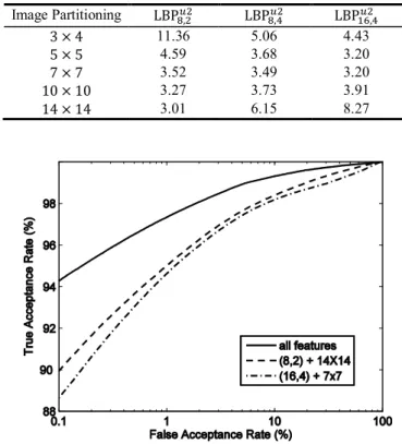
In the final experiment, we explored the capability of the classification framework for fusing different sources of facial information. To do that, various image partitionings and LBP operators were used to extract a range of feature sets. The framework was then tested for all the three LBP feature types on each of the seven image partitionings. Table 3 shows the average EERs calculated for each combination. The resulting features were then concatenated to produce fused features used for classification. Fig. 6 presents the results in terms of ROC curves. Besides the ROC for all features, the figure also shows the ROC curves for the two kinds of features with the smallest EERs. It can be seen that the classification framework not only can handle each of the different kinds of features, but is capable of fusing the facial information carried by the features to give a much better performance.
5 Conclusions
In this paper, a generic classification framework has been proposed for large-scale face recognition systems. The framework consists of two components: a data sampling strategy and a modified kernel Fisher discriminant classifier. The sampling strategy is aimed at dealing with the imbalance within the large amount of training data when image pairs are sampled for feature extraction. The modified KFD provides a simple solution for using the KFD algorithm given a large training dataset. Various experiments have been carried out in an open-set scenario and results suggest that the classification framework can provide an effective solution in terms of accuracy and computational efficiency.
References
1. Ahonen, T., Hadid, A., Pietikäinen, M.: Face description with local binary pattern: Application to face recognition. TPAMI, 28(12): 2037-2041 (2006)
2. Beveridge, J. R., Bolme, D. S., Draper, B. A., Teixeira, M.: The CSU face identification evaluation system: its purpose, features, and structure. Machine Vision and Applications, 16(2):128–138 (2005)
3. Joachims, T.: Making large-scale SVM learning practical. In: Advances in Kernel Methods - Support Vector Learning. MIT Press, Cambridge, MA (1998)
4. Jonsson, K., Kittler, J., Li, Y., Matas, J.: Support Vector Machines for Face Recognition. In: BMVC’99, pp. 543-553, Nottingham, UK (1999)
5. Mika, S., Rätsch, G., Weston, J., Schölkopf, B., Muller, K. R.: Fisher discriminant analysis with kernels. In: Proceedings of the 1999 IEEE Signal Processing Society Workshop, pp. 41–48, IEEE Press, Piscataway, NJ (1999)
Table 3. Average EERs (%) calculated using different image partitioning and LBP operators. Image Partitioning LBP, LBP, LBP , 3 × 4 11.36 5.06 4.43 5 × 5 4.59 3.68 3.20 7 × 7 3.52 3.49 3.20 10 × 10 3.27 3.73 3.91 14 × 14 3.01 6.15 8.27
Fig. 6. ROC curves for the fused features and two individual features with the smallest EERs.
6. Moghaddam, B., Wahid, W., Pentland, A.: Beyond Eigenfaces: probabilistic matching for face recognition. In: FG’98, pp. 14-16 (1998)
7. Phillips, P. J.: Support vector machines applied to face recognition. In: Proceedings of Advances in Neural Information Processing Systems II, pp. 803-809 (1999)
8. Phillips, P. J., Grother, P., Micheals, R. J., Blackburn, D. M., Tabassi, E., Bone, M.: Face recognition vendor test 2002: overview and summary. (2003)
9. Phillips, P. J., Flynn, P. J., Scruggs, W. T., Bowyer, K. W., Chang, J., Hoffman, K., Marques, J., Min, J., Worek, W.: Overview of the face recognition grand challenge. In CVPR, pp. 947–954, San Diego, CA (2005)
10.Phillips, P. J., Scruggs, W. T., O’Toole, A. J., Flynn, P. J., Bowyer, K. W., Schott, C. L., Sharpe, M.: FRVT 2006 and ICE 2006 Large-Scale Results. TR-NISTIR 7408 (2007) 11.Schölkopf, B., Smola, A. J.: Learning with Kernels: Support Vector Machines,
Regularization, Optimization, and Beyond. MIT Press, Cambridge, MA (2001)
12.Snelick, R., Uludag, U., Mink, A., Indovina, M., Jain. A.: Large-scale evaluation of multimodal biometric authentication using state-of-the-art systems. TPAMI, 27(3): 450 – 455 (20005)
13.Yang, J., Frangi, A. F., Yang, J., Zhang, D., Jin, Z.: KPCA Pluse LDA: a complete kernel Fisher discriminant framework for feature extraction and recognition. TPAMI, 27(2), 230 – 244 (2005)
14.Zhao, W., Chellappa, R., Rosenfeld, A., Phillips, P. J.: Face Recognition: A Literature Survey, ACM Computing Surveys. 399-458 (2003)