Highly efficient distributed hypergraph analysis: real-time partitioning and quantized learning

Highly Efficient Distributed

Hypergraph Analysis: Real-time

Partitioning and Quantized Learning

Wenkai Jiang

orcid.org/0000-0001-6791-4307

Submitted in total fulfilment of the requirements of the degree of

Master of Philosophy

School of Computing and Information Systems THEUNIVERSITY OF MELBOURNE

All rights reserved. No part of the publication may be reproduced in any form by print, photoprint, microfilm or any other means without written permission from the author.

Abstract

Hypergraphs have been shown to be highly effective when modeling a wide range of applications where high-order relationships are of interest, such as social network analysis and object classifi-cation via hypergraph embedding. Applying deep learning techniques on large scale hypergraphs is challenging due to the size and complex structure of hypergraphs. This thesis addresses two problems of hypergraph analysis, real-time partitioning and quantized neural networks training, in a distributed computing environment.

When processing a large scale hypergraph in real-time and in a distributed fashion, the quality of hypergraph partitioning has a significant influence on communication overhead and workload balance among the machines participating in the distributed processing. The main challenge of real-time hypergraph partitioning is that hypergraphs are represented as a dynamic hypergraph stream formed by a sequence of hyperedge insertions and deletions, where the structure of a hy-pergraph is constantly changing. The existing methods that require all information of a hyhy-pergraph are inapplicable in this case as only a sub-graph is available to the algorithm at a time. We solve this problem by proposing a streaming refinement partitioning (SRP) algorithm that partitions a real-time hypergraph flow in two phases. With extensive experiments on a scalable hypergraph framework named HyperX, we show that SRP can yield partitions that are of the same quality as that achieved by offline partitioning algorithms in terms of communication overhead and workload balance.

For machine learning tasks over hypergraphs, studies have shown that using deep neural net-works (DNNs) can improve the learning outcomes. This is because the learning objectives in hypergraph analysis are becoming more complex these days, where features are difficult to define and are highly-correlated. DNNs can be used as a powerful classifier to construct features automat-ically. However, DNNs require high computational power and network bandwidth as the size of

the broadcasts of parameters during the partial gradient aggregations, and the inherent variance between partial gradients, making the training process even longer as it impedes the convergence rate of SGD. We investigate these two problems in depth. Without sacrificing the performance, we develop a quantization technique to reduce the communication overhead and a new training paradigm, named cooperated low-precision training (C-LPT), in which importance sampling is used to reduce variance, and the master and workers collaborate together to make compensation for the precision loss due to the quantization.

Incorporating deep learning techniques into distributed hypergraph analysis shows a great po-tential in query processing and knowledge mining on high-dimensional data records where rela-tionships among them are highly correlated. On one hand, such a process takes the advantage of strong representational power of DNNs as an appearance-based classifier; on the other hand, such a process exploits hypergraph representations to gain benefits from its strong capability in capturing high-order relationships.

Declaration

1. the thesis comprises only my original work towards the MPhil except where indicated, 2. due acknowledgment has been made in the text to all other material used,

3. the thesis is less than 50,000 words in length, exclusive of tables, maps, bibliographies and appendices.

Wenkai Jiang, September 2018

Acknowledgements

First and foremost, I would like to express the depth of my gratitude to my supervisors Professor Rui Zhang and Doctor Jianzhong Qi. They are brilliant researchers and advisers that lead me into this exciting field of developing techniques for distributed processing. They have always been very supportive during my study. Without their continuous help, trust, and encouragement, I would not have opportunities to pursue my own research interests and this degree would never be possible.

Next, I want to thank my advisory committee chair, Doctor Sean Maynard, for spending his time in giving me advice and guidance on building my study plan and providing valuable feedback on many matters.

I am also very grateful to my external advisor Doctor Wei Wang. I feel very fortunate to have him as an advisor as well as a friend. He not only taught me many technical skills in approaching research problems, but also helped me a lot in my life during the time I spent in Singapore. He gave me numerous constructive suggestions on quantized deep neural network training. I enjoyed those discussions with him and his insightful feedbacks have been invaluable to my research.

Thanks also due to all colleagues in our research group, especially Jin, Yiqing, Andy, Yu, Zeyi, Xiaojie, Chuandong, Saad, Jiazhen, Yuan, Gitansh, Han, He, Weihao, Xinting. They have been good friends in my life in Melbourne and many of them have provided me invaluable advice.

I own the best truly sincere gratitude to my parents, who have given me unconditional love and care all the time. Whenever I run into problems, they have always been trying to take me under their wings to make me warm and to help me get through. Without their support, I would not be able to achieve where I am today.

Last but not least, I am very thankful to the University of Melbourne, to the School of Com-puting and Information System, and to the Melbourne Research Scholarships, for providing the financial support for both of my education and the research in this thesis.

Preface

The work on scalable hypergraph learning, presented in Chapter 3, has been accepted for publica-tion: Jiang, W., Qi, J., Yu, J., Huang, J., and Zhang, R. (2018). HyperX: A scalable hypergraph framework. IEEE Transactions on Knowledge and Data Engineering.

Contents

1 Introduction 1

1.1 Motivation on Hypergraph Representations . . . 4

1.1.1 Hypergraph Representation . . . 4

1.1.2 Conversion between Graphs and Hypergraphs . . . 5

1.2 Motivation of Quantization in Deep Neural Networks . . . 7

1.3 Distributed Data Processing . . . 9

1.3.1 Computational Paradigms . . . 10

1.3.2 Challenges in Distributed Computing . . . 11

1.4 Thesis Contributions . . . 12

1.4.1 Publication Out of This Thesis . . . 13

1.5 Thesis Outline . . . 14

2 Literature Review 15 2.1 Graph and Hypergraph Partitioning . . . 15

2.1.1 Graph Partitioning . . . 16

2.1.2 Graph Partitioning with Heuristics . . . 17

2.1.3 Streaming Graph Partitioning . . . 18

2.1.4 Hypergraph Partitioning . . . 19 xi

2.2.1 Deep Learning . . . 20

2.2.2 Neural Network Architectures . . . 23

2.3 Quantized Neural Network Training . . . 26

3 Real-time Hypergraph Partitioning for Distributed Learning 29 3.1 Introduction . . . 29

3.2 Preliminaries . . . 31

3.2.1 HyperX: Scalable Hypergraph Framework . . . 31

3.2.2 Semi-supervised Learning via Label Propagation . . . 34

3.3 Partitioning Objective and Theoretical Analysis . . . 35

3.3.1 Partitioning Objective . . . 35

3.3.2 The Strict Case . . . 37

3.3.3 A Variant with Soft Constraints . . . 38

3.4 Streaming Refinement Partitioning (SRP) . . . 39

3.4.1 Rough Partitioning . . . 40

3.4.2 Iterative Refinement . . . 41

3.5 Experiments . . . 45

3.5.1 Experimental Settings . . . 45

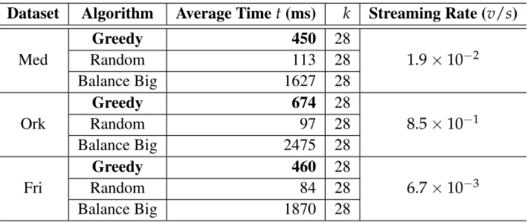
3.5.2 Partitioning Time of Partitioning Algorithms . . . 49

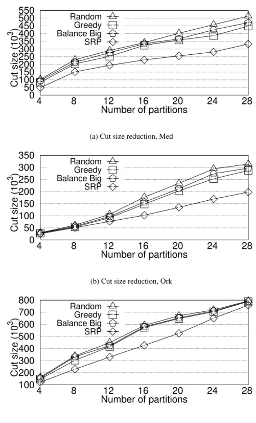
3.5.3 Cut Size of Partitioning Algorithms . . . 50

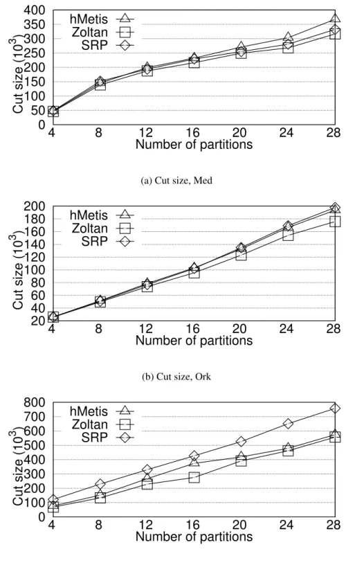
3.5.4 Quality of Partitioning of Hypergraph Learning Algorithms . . . 53

3.6 Summary . . . 56 xii

4 Distributed Neural Network Training with Quantization 59

4.1 Introduction . . . 59

4.2 Preliminaries . . . 62

4.2.1 Synchronous SGD Parallelization and Communication Overhead . . . 62

4.2.2 Importance Sampling . . . 64

4.3 Cooperated Low Precision Training (C-LPT) . . . 68

4.3.1 Gradient Quantization . . . 68

4.3.2 Gradient Aggregation with Various Precision . . . 79

4.3.3 Training Batch Sampling . . . 91

4.4 Experiments . . . 94

4.4.1 Experimental Settings . . . 95

4.4.2 Evaluation on the Impact of Gradient Quantization . . . 96

4.4.3 Evaluation on Gradient Aggregation with Various Precisions . . . 99

4.4.4 Evaluation of Importance Sampling on Training Batches . . . 102

4.5 Summary . . . 105

5 Conclusions and Future Work 107 5.1 Conclusions . . . 107

5.2 Future Work . . . 109

Bibliography 111

List of Figures

1.1 Converting a hypergraph to a graph: CE and SE . . . 5

2.1 A neural network with one hidden layer . . . 22

2.2 LeNet-5 Architecture [78] . . . 24

2.3 AlexNet Architecture [74] . . . 25

2.4 VGG-16 Architecture [105] . . . 25

2.5 ResNet Architecture [47] . . . 26

2.6 DeepSpeech Architecture, DeepSpeech 1 on the left [46] and DeepSpeech 2 on the right [2] . . . 26

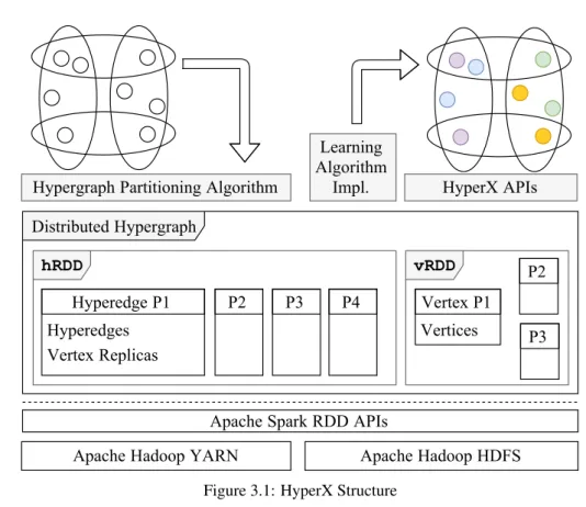
3.1 HyperX Structure . . . 32

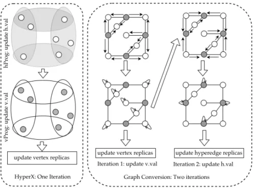
3.2 Comparing HyperX with Graph Conversion, the gray shapes and bold arrows in-dicate the running ofvProgandhProgin each step . . . 33

3.3 Evaluate the cut size reduction from rough partitioning to SRP . . . 51

3.4 Comparing cut size of SRP with offline partitioning algorithms . . . 52

3.5 Comparing the space cost of partitioning algorithms . . . 54

3.6 Comparing the workload balance . . . 54

3.7 Comparing the communication cost of partitioning algorithms . . . 55

3.8 Comparing the elapsed time . . . 55

4.1 Illustration of an application combining hypergraphs and DNNs [56] . . . 60

4.2 Parallel SGD Training. . . 64

4.3 Quantized distributed training with multiple GPUs on multiple nodes. . . 65

4.4 Cooperated low precision training (C-LPT) with multiple GPUs on multiple nodes. 68 4.5 Comparison of communication time and computation time in one iteration on AlexNet when the number of nodes varies . . . 69

4.6 Illustration of back-propagation algorithm . . . 70

4.7 Gradients updates based on weights clustering and gradients grouping [45] . . . . 74

4.8 Stochastic Quantization [36] . . . 76

4.9 Distribution of gradients at convolutional layer after training AlexNet for 50 iter-ations . . . 77

4.10 Gradient aggregation with different precision gradient matrix on master side . . . 80

4.11 Illustration of bit centering [26] technique . . . 89

4.12 Illustration of importance sampling . . . 93 4.13 Learning curves of SVRG and Fixed Coefficient Values on ResNet with Cifar10 . 98 4.14 Learning curves of IAGA with and without bit centering on ResNet with Cifar10 100

List of Tables

1.1 Hypergraph Applications . . . 3

3.1 The APIs ofHypergraph[V, H]in HyperX . . . 35

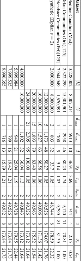
3.2 Comparison on the size of datasets . . . 46

3.3 Datasets presented in the empirical study . . . 47

3.4 Partitioning time with online algorithms . . . 50

3.5 Partitioning time with offline algorithms . . . 50

4.1 Comparison of the error rate (%) of SGD after sign and magnitude modification with P=0.75 . . . 71

4.2 Volume of message sent over network . . . 96

4.3 Comparing training throughput on GPU cluster . . . 97

4.4 Comparison of gradient aggregation on ImageNet with AlexNet and VGG-16 . . 99

4.5 Evaluation of IAGA on ImageNet with AlexNet and VGG-16 . . . 101

4.6 Training results of speech recognition with RNN . . . 102

4.7 Number of data points by hardness in classification on MNIST and Cifar-10 . . . 104

4.8 Comparison of ISGD and SGD . . . 104

Chapter 1

Introduction

Hypergraphs have attracted many attentions during the past few years and have been applied to a wide range of applications such as social network analysis [132], image retrieval [55, 138], object classification [40], facial emotion recognition [56], and image segmentation [54]. Among these applications, data records are obtained from either online streaming or offline collections and modeled as hypergraphs for learning. Due to the huge success of deep learning techniques in many machine learning tasks, recent studies start combining deep neural networks (DNNs) with learning tasks on hypergraphs to achieve better performance. For example, deep learning has been used for creating embeddings of a social network represented as a hypergraph [87, 134]. This is to represent each vertex of a hypergraph in a latent lower dimensional space. After embeddings are created, DNNs can be applied once again to learn the relationships between these vertices from its own embeddings and embeddings of other vertices.

Thanks to the rapid development of the Internet, a huge amount of data is generated and col-lected at an unprecedented speed from all aspects of life, such as online social media, public health care systems or retail stores. The amount of available data in these areas has exploded significantly in the past decades also because of the fast growing number of applications and users. As a result, when modeling these data into hypergraphs, the size of hypergraphs has become larger. Analysis over these large scale hypergraphs poses new challenges in computational capabilities. It is com-mon to use a cluster of distributed computers to solve learning problems on larger hypergraphs.

In this thesis, we investigate hypergraph processing and deep learning tasks on hypergraphs in the context of distributed computing. In particular, this thesis addresses two problems of hy-pergraph analysis, real-time partitioning and quantized neural networks training, in a distributed computing environment. Hypergraphs have been shown to be highly effective when modeling a

wide range of applications where high-order relationships are of interest. Applying deep learn-ing techniques on large scale hypergraphs is challenglearn-ing due to the size and complex structure of hypergraphs. For machine learning tasks over hypergraphs, studies have shown that using DNN can improve the learning outcomes. This is because the learning objectives in hypergraph analysis are becoming more complex these days, where features are difficult to define and are highly-correlated. DNNs can be used as a powerful classifier to construct features automatically. Hypergraph analysis using the combination of hypergraphs and DNNs can be found in many ap-plications these days and achieves a remarkable success. For example, when detecting emotions of a person [56], facial images firstly pass through a convolutional neural network to be decom-posed into several hidden expression features; next, high-order relationships between emotional features are depicted by hyperedges for emotion prediction. On one hand, such a process takes the advantage of strong representational power of DNNs as an appearance-based classifier; on the other hand, such a process exploits hypergraph representations to gain benefits from its strong capability in capturing high-order relationships. Incorporating deep learning techniques into dis-tributed hypergraph analysis shows a great potential in query processing and knowledge mining on high-dimensional data records where relationships among them are highly correlated.

Hypergraphs have been used to represent the data records with full of rich structures and high-dimensional relationships among many applications. In these applications, the data records are represented by vertices and the relationships between data records are modeled as hyperedges. When applications involve huge amount of data, the size of hypergraph can be very large. Min-imizing the query cost on such hypergraphs is crucial for the applications. For example, when querying a social network represented as a hypergraph for users’ activities, real-time analytics re-quires low latency between sending queries and receiving results so that users do not experience a long waiting time. For a hypergraph representing millions of users and relationships, partition-ing strategy is critical to reduce the latency. In this scenario, hypergraph partitionpartition-ing helps to partition the query loads to several workers, which enables horizontal scaling of the large-scale hypergraphs.

Hypergraphs analysis requires first establishing a learning goal. However, as the structure of hypergraph is becoming more complicate, the size of hypergraph is getting bigger, and the applica-tion scenarios are becoming more diverse, it is becoming more difficult to establish these learning

3 Table 1.1: Hypergraph Applications

Application Algorithm Vertex Hyperedge

Recommendation [110] Songs and users Listening histories

Text retrieval [52] Documents Semantic similarities

Image retrieval [84] Images Descriptor similarities

Multimedia [109] Videos Hyperlinks

Bioinformatics [59] Proteins Interactions

Social mining [111] Users Communities

Machine Learning [120] Records Labels

goals. In particular, it is difficult to manually select or craft features on the hypergraphs as they are mostly highly related to each other. Deep neural networks (DNNs) can automatically generate these features by learning on a large number of hypergraphs. DNNs is a deep learning technique that has brought substantial advances to a wide range of applications that are driven by large-scale data sets and sophisticated models. However, training distributed DNNs is difficult to scale due to the inequality between computing time and communication time. The computation time can be significantly reduced by adding more workers to the cluster. However, the overhead of gradient synchronization increases dramatically along with the growth of number of workers [81]. The larger the scale of the distributed system, the more severe the bottleneck of the communication will be. Eventually this would offset the savings of computing power [80]. To tackle this com-munication bottleneck, model compression techniques [45, 57, 83, 91, 121, 136] such as sparse and quantized DNNs have been studied forinferencetasks. The speed and efficiency ofinferencegain huge benefits from the use of modern hardware accelerators such as Google’s TPU [63]. How-ever, these accelerators are mainly used ininferencebut nottrainingas the influence of reducing precision duringtraininghas not been fully investigated.

We investigate how to use the widely-deployed distributed cluster to realize real-time hyper-graph partitioning, and achieve high scalability in DNNs training for hyperhyper-graph analysis. We propose techniques in hypergraph partitioning and neural network training to both ease the imple-mentation and boost the computation. These techniques can be easily adopted by other distributed applications.

In the remainder of this chapter, we first describe the motivation of using hypergraph rather than normal graph to represent high-order relationships. Next, we elaborate the motivation of adopting quantization technique in deep neural networks training. After that, we briefly describe

the context of distributed computation over a cluster of commodity machines and its challenges. Last, the contributions of this thesis are summarized and the thesis outline is shown.

1.1

Motivation on Hypergraph Representations

Graphs allow each edge to connect two vertices representing a certain relationship between them. For example, in a map of a city, an edges connecting two vertices may represent a path between two locations. In a wide range of applications, a relationship may be formed by more than two objects. For example, a picture posted by a user on a social network is likely to be liked by multiple of his friends; a tweet may be reposted by many users who have read it. In such applications, modeling objects and their relationships with a graph may incur information loss [134]. A common approach to address this problem is representing the objects and their relationships by vertices and hyperedges in a hypergraph. A hypergraph is a generalized graph where an edge can connect more than two vertices. Hypergraph models have shown great effectiveness in capturing high-order relationships [52,59,84,109–111,120]. Table 1.1 summarizes some representative examples of hypergraph applications.

1.1.1 Hypergraph Representation

We denote a hypergraph as G = hV,Hi, where V = {v1,v2, . . . ,vm} is a set of m vertices

andH = {h1,h2, . . . ,hn}is a set ofnhyperedges. Thedegreeof a vertex v, denoted by dv, is

the number of hyperedges that are incident tov. The arityof a hyperedgeh, denoted by ah, is the number of vertices inh, i.e., the number of vertices that are incident toh. Every vertexvand every hyperedgehis associated with some attributes of interest called a vertex value (e.g., a label), denoted byv.valand a hyperedge value (e.g., a weight), denoted byh.val, respectively.

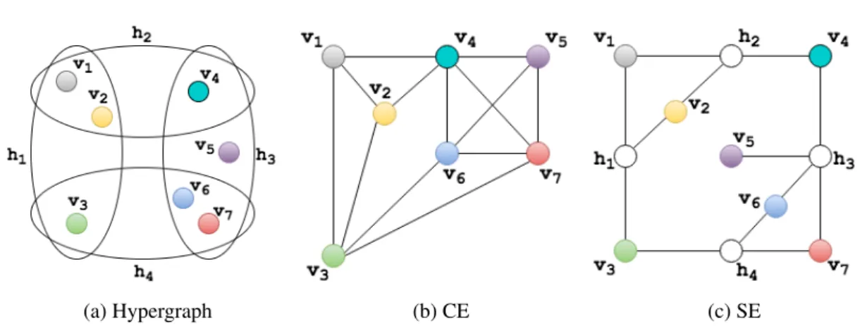
Both undirected and directed hyperedges are considered. An undirected hyperedge h is a nonempty subset ofV. For example, in Fig. 1.1a, there are four undirected edges,h1,h2,h3and h4, represented by four ellipses. Each is a subset ofV ={v1,v2, . . . ,v7}, e.g.,h1 ={v1,v2,v3}.

Since there are three vertices in h1, thearityofh1is 3, i.e., ah1 = 3. Meanwhile, sincev1 is in

1_{Part of this section has been published in: Jiang, W., Qi, J., Yu, J., Huang, J., and Zhang, R. (2018). HyperX: A}

1.1 Motivation on Hypergraph Representations 5

(a) Hypergraph (b) CE (c) SE

Figure 1.1: Converting a hypergraph to a graph: CE and SE

bothh1andh2, itsdegreeis 2, i.e.,dv1 =2. A directed hyperedgehis a mapping on two disjoint

nonempty vertex sets ofV: a source setS and a destination setD, i.e.,h :S → D. For example, in Fig. 1.1a, we can change hyperedgeh1 to a directed hyperedge by assigning {v1,v2} as the

source set and{v3}as the destination set, i.e.,h1:{v1,v2} → {v3}.

1.1.2 Conversion between Graphs and Hypergraphs

While applications of hypergraphs are emerging, there has been little work on developing a frame-work to support hypergraph representation directly. Graph frameframe-works cannot process hyper-graphs without converting hyperhyper-graphs into hyper-graphs. Converting a hypergraph into a graph may inflate the size of the original hypergraph, because every hyperedge needs to be replaced by a clique which increases the number of edges and vertices. For example, a hypergraph studied pre-viously [125] with 2 million vertices and 15 million hyperedges is converted to a bipartite with 17 million vertices and 1 billion edges. Such inflation causes huge difficulty in processing the hypergraph.

Two traditional graph representations are used for converting a hypergraph into a graph [134]: 1)clique-expansion (CE), which replaces each hyperedge with multiple edges forming a clique among the incident vertices of the hyperedges, and 2)star-expansion(SE), which replaces each hyperedge with a new vertex connected to its incident vertices. Fig. 1.1 illustrates these two approaches where the hypergraph in Fig. 1.1a is converted to a graph shown in Fig. 1.1b by CE and a graph shown in Fig. 1.1c by SE, respectively. Although these approaches are simple to implement, they have substantial limitations.

1. CE is inapplicable to algorithms that update hyperedge values as it no longer has records corresponding to the original hyperedges in the converted graph.

2. The converted graph may have orders of magnitude more vertices and edges compared with the original hypergraph. Fig. 1.1 shows a substantial growth even in a tiny hypergraph. The hypergraph with 4 hyperedges and 7 vertices is converted by CE into a graph with 13 edges and 7 vertices and by SE into a graph with 13 edges and 11 vertices.

3. For SE, there are two types of vertices, those from the original hypergraph and those con-verted from the hyperedges of the original hypergraph. Two vertex programs are used for updating these two types of vertices. When executing these two vertex programs, it takes two iterations to update the vertex values and hyperedge values, which is a drawback, be-cause the two iterations double the overhead of updating the vertex replicas.

To partition a streaming hypergraph directly using hypergraph representation, we partition it using a recently proposed hypergraph framework, HyperX . HyperX is a thin layer built upon Apache Spark [128]. It provides flexible and expressive interfaces for the ease of implementation of hypergraph learning algorithms, operating directly on the hypergraph representation. To ease the use of the framework, HyperX provides ahyperedge programand avertex programwhich are consistent with theedge programandvertex programused in popular graph frameworks such as GraphX. HyperX uses the Bulk Synchronous Parallel (BSP) message passing scheme, which is commonly used in synchronous graph processing frameworks.

HyperX builds a foundation that supports processing hypergraphs at large scale. When hyper-graphs are large, HyperX distributes the computation over across many workers. This calls for a hypergraph partition algorithm to create partitions that can be processed in a distributed man-ner with a balanced workload and low communication costs among the workers. The efficiency of a hypergraph processing algorithm running on HyperX may be significantly impacted by the hypergraph partitions.

1.2 Motivation of Quantization in Deep Neural Networks 7

1.2

Motivation of Quantization in Deep Neural Networks

Hypergraphs have been shown to be highly effective when modeling a wide range of applications where high-order relationships are of interest. Applying deep learning techniques on large scale hypergraphs is challenging due to the size and complex structure of hypergraphs. For machine learning tasks over hypergraphs, studies have shown that using deep neural network (DNN) can improve the learning outcomes. This is because the learning objectives in hypergraph analysis are becoming more complex these days, where features are difficult to define and are highly-correlated. DNNs can be used as a powerful classifier to construct features automatically. Hyper-graph analysis using the combination of hyperHyper-graphs and DNNs can be found in many applications these days and achieves a remarkable success. For example, when detecting emotions of a per-son [56], facial images are firstly passed through a convolutional neural network to be decomposed into several hidden expression features; next, high-order relationships between emotional features are depicted by hyperedges for emotion prediction. Another example is to create hypergraph em-beddings using DNNs [87, 134]. This is to represent each vertex of a hypergraph in a latent lower dimensional space. After embeddings are created, DNNs can be applied once again to learn the relationships between these vertices from its own embeddings and embeddings of other vertices.

On one hand, such a process takes the advantage of strong representational power of DNNs as an appearance-based classifier; on the other hand, such a process exploits hypergraph representa-tions to gain benefits from its strong capability in capturing high-order relarepresenta-tionships. Incorporating deep learning techniques into distributed hypergraph analysis shows a great potential in query pro-cessing and knowledge mining on high-dimensional data records where relationships among them are highly correlated.

For distributed hypergraph analysis with deep learning techniques, the performance of the whole work flow depends not only on the hypergraph processing itself, but also on the performance of the DNNs, including phases of training and inference. Training distributed DNNs is known to be difficult to scale due to the inequality between computing time and communication time. Poor scalability will greatly damaged the efficiency of the whole system.

During the past few years, DNNs have been rapidly developed in various applications. Scaling up neural networks with respect to the number of parameters has significantly raised the state-of-the-art performance in several fields, including image classification, speech recognition, and

arti-ficial intelligence, such as AlphaGo [103] playing against professional players. The performance gain of these DNNs generally comes with high computational costs and large memory consump-tion, which may not be affordable for mobile platforms. Quantization is originally proposed to compress the deep neural network models in order to reduce the computation and storage costs of DNNs so that complex DNNs can be deployed on portable devices, such as mobile phones. Except for the need in portable device deployment, quantization can also be used to compress gra-dients to reduce communication overhead. In the training phase, the parallelization of stochastic gradient descent (SGD) requires synchronizations to gather gradients and parameters for aggre-gation in each iteration, and this introduces significant communication overhead. Using gradient quantization may reduce the communication overhead by tens of times.

If energy consumption is monitored for each operation when training DNNs, it is reported that communication counts for a significant fraction among various sources. Communication takes up to 50% of the power consumption in a multi-GPUs configuration of a state-of-the-art DNN training scheme [21]. This number includes the energy needed for data I/O on external and internal memories. It also includes energy for communicating values across the distributed systems.

The need to improve performance and reduce the communication overhead for DNNs is a hot research topic in recent years. The most popular approach is to use reduced precision represen-tation for the numerical data compurepresen-tation. The most aggressive reduction in precision turns the whole model into a binarized neural network (BNN). BNN constrains both the weights and the activation to be either +1or −1. It is claimed that these two values are extremely suitable for hardware optimization. Two different binarization functions have been proposed [24] to transform the full-precision variables into these two values.

Even though BNN utilizes binary weights and activation functions to compute gradients, the gradients that are aggregated to update the weights are in full precision. This is because it was believed that full-precision gradients are required for SGD to work properly. SGD explores the direction of gradients in small and noisy steps and the noise is offseted by the stochastic gradient aggregated in each step. As a result, it is critical to keep gradients in full precision. This actually is found not correct by recent work [82], which shows that gradients have very similar characteristic as weights, wheresignmatters more thanmagnitude. Thus, the gradients can be safely quantized as well.

1.3 Distributed Data Processing 9 Moreover, the noise of gradients provides a form of regularization that can help deep neural network models to generalize better. Quantization of the gradients is equivalent to adding more noise to the system. In this sense, previous techniques that have been widely adopted in modern DNNs training can be merged in without modifications, such as Dropout [106] and DropCon-nect [118].

An issue to be noticed is that, since the derivative of the sign function is zero almost every-where, it can not be used for back-propagation (BP). Bengio et al. [10] study the problem of training stochastic discrete neurons using quantized gradients. The finding is that fastest training can be obtained by using the “straight-through estimator”. All these factors motivate us to incor-porate data quantization into the DNNs training and inference phase to make the operations more efficient on either desktop or portable devices.

1.3

Distributed Data Processing

Distributed computing on a cluster of machines can be deployed in different ways, e.g., the Mes-sage Parssing Interface (MPI), the Parallel Random Access Machine (PRAM), and MapReduce based platform (Hadoop2). In recent years, the MapReduce based platform becomes popular for applications with large scale of data that cannot be held by a single machine.

There are many implementations of the map-reduce computing paradigm. Hadoop is the most popular one among them, and it is more than just MapReduce. Hadoop provides three basic components: the storage engine called the Hadoop Distributed File System (HDFS); the resource manager named the Yet Another Resource Negotiator (YARN), and the computational paradigm, MapReduce. Apache Spark3can re-use the HDFS and YARN while it substitutes the MapReduce with a more advanced computational engine, which provides more operations including filter, join, and more importantly, it runs in memory, unlike Hadoop which is on disk. The three compo-nents in Hadoop is loosely-coupled, which makes them easy to be replaced by other counterparts correspondingly, such as Amazon S3 file system, Apache Mesos resource manager, Apache Hama computational framework. Plugging and unplugging different storage engines, resource managers, and computational engine is convenient. As an open source implementation, Hadoop provides an

2_{Apache Hadoop, Apache Software Foundation, available at https://hadoop.apache.org/} 3_{Apache Spark, Apache Software Foundation, available at https://spark.apache.org/}

assembly of distributed systems to make it look like an operating system running on a single ma-chine. In the following subsections, we describe three computational paradigms that are widely used in distributed computing.

1.3.1 Computational Paradigms

Three basic components in Hadoop execute in a master-slave fashion to organize the cluster. This is to parallel the computation to all the slave machines at the first, and synchronize the result on master via network communication among the slaves. There are three main computation paradigms.

BSP Paradigm [116].BSP contains a series of super-steps. In each super-step, only a subset of the data is used to compute. This subset of data firstly compute locally on every slaves, and then the result is combined with the messages received from last super-step to generate a bunch of new messages. Finally, these new generated messages are send to particular machines. After that, this cycle repeats. There is a synchronization step between each super-step, which guarantees that all messages are received from senders. Because of the synchronization, the overall speed depends on the slowest machine.

MapReduce [29]. Unlike BSP, MapReduce do not have super-step. On the other hand, each step of it has two phases, map andreduce. The map groups data records based on a user de-fined key, and thereduce aggregate data records sharing the same key based on a user defined reduce function. Bothmapandreduceexecutes on each machine independently. And there is one synchronization step betweenmapandreduce.

Spark [128].Different from above two paradigms, Spark use a directed acyclic graph (DAG) to determine the order of operations that will be executed on the partitioned data. And it adopts lazy evaluation to make real computation as late as possible. Each vertices in the DAG represents the operations that could be run independently on the distributed system and each edge connects two vertices to denote the source and destination of message passing over the network. There is one synchronization barrier between two connected vertices. Spark is faster than previous two by several magnitudes due to its memory running environment and lazy evaluation.

1.3 Distributed Data Processing 11 1.3.2 Challenges in Distributed Computing

When developing hypergraph processing algorithms and deep neural network training over a distributed system, the challenges lie in intensive computation, difficulty in balancing the work-load, and communication overhead minimization.

Intensive Computation. A hypergraph with billions of vertices and hyperedges need to be partitioned to the distributed machines. Partitioning algorithms that have theoretical quality guar-antee, e.g., semi-definite programming based solution, or good approximation properties, e.g., spectral clustering based solution, are prohibitive when confronting a large scale hypergraph [53]. For streaming hypergraph partitioning, only partial structure information is known. This makes partitioning even harder. So effective streaming hypergraph partitioning algorithm need to be designed.

As for deep neural networks (DNNs) training, a model can easily have millions parameters. Thanks to the remarkable development with GPU chips, the short of computational power has been remedied to some extents, but still as the model becomes larger, there is a great need in developing a low computational cost model.

Difficulty in Balancing Workload. Both hypergraph partitioning over Hadoop and DNNs training have synchronization barrier and need to wait for the slowest machine to complete the computation. Therefore, the balanced workload is essential to the efficiency of both applications. In hypergraph processing, because two hyperedges may overlap over several vertices, these ver-tices are therefore replicated several times. As a result, workload balancing in hypergraph parti-tioning not only need to consider the existing vertices in the hypergraph, but also need to optimize which vertices should be replicated and where to partition those replications to.

Communication Overhead. There is a trade-off between workload balancing and optimum communication. Take two extreme cases into consideration: there is no communication overhead if there is only one partition of data records, where the workload is totally unbalanced; there will be arbitrarily high communication overhead if data records are partitioned randomly into all workers, where the workload is absolutely balanced. When a hypergraph is partitioned, the fundamental rule is that partitioning should maintain the tightly nested sub-hypergraph so that natural clusters are partitioned near to each other. This would significantly reduce the unnecessary replicas and

communication overhead. Conversely, when training DNNs, this partitioning strategy does not work because there is no natural connection between data points. So to minimize communication overhead in DNNs training, we have to consider model compression or gradient quantization.

1.4

Thesis Contributions

We describe the contributions of this thesis in the real-time hypergraph partitioning on HyperX and the quantized deep neural network training. Regarding to the challenges discussed in Section 1.3.2, the communication challenges are intended to solve in both studies, while the computational and workload balance challenges are mainly reflected in the algorithm design in real-time hypergraph partitioning.

Our contributions on real-time hypergraph partitioning are:

• We investigate the real-time hypergraph partitioning problem where vertices arrive one at a time in a sequential manner. We formulate it as an integer programming problem to mini-mize the number of replicas during the partitioning, therefore minimini-mize the communication costs when running hypergraph applications.

• We design a streaming refinement partitioning (SRP) algorithm which partitions a stream-ing hypergraph streamstream-ing in two steps. In the first step, rough partitionstream-ing, we investigate practical heuristics and propose a greedy strategy to create fast and rough partitions. In the second step, iterative refinement, we use label propagation with a fixed size sliding window to make the streaming partitioning algorithm independent of the streaming length in order to comply with the time and memory constraints in real-time processing.

• We evaluate SRP against a number of online and offline partitioning algorithms with ex-tensive experiments on both real datasets and synthetic datasets. The results demonstrate that SRP is suitable for streaming partitioning as the average partitioning time is smaller than streaming rate. The results show that SRP not only deliver better partitioning results in terms of cut size and work-load balance compared to that of offline partitioning algorithms, but also delivered more efficient and effective performance when running hypergraph learn-ing algorithms

1.4 Thesis Contributions 13 Our contributions on quantized deep neural network training are:

• We investigate methods to incorporate deep learning techniques into distributed hypergraph analysis. We design a cooperated low precision training (C-LPT) paradigm for deep neural network training. In C-LPT, we allow masters and workers to keep two different sets of a model in different precision level. In each training iteration, the workers are trained on a low-precision model using a large batch size, while masters are trained on a small portion of the batch (which are sampled from the large batch size trained on workers) with a high-precision model.

• We investigate quantization methods and design a logarithmic quantization method with two factors. Instead of using full-precision (i.e., 32-bit floating points) representation, we restrict the values of parameters on workers to be either powers of two or zero. To minimize the error caused by quantization, a re-scaling strategy calledbit centering[26] is integrated in our algorithm. In this way, the error of quantization will converge to zero asymptotically. • We explore approaches to reduce the variance in training data points and we extend C-LPT to adopt importance sampling for variance reduction. In C-C-LPT, importance sampling happens only when sampling a subset of the training batch on workers to be trained on the master side. This particular batch on the worker side is uniformly sampled from the whole dataset.

• We conduct extensive experiments using C-LPT with various neural network architectures and real datasets. The results demonstrate that C-LPT can benefit DNN training in two folds. Firstly, the communication overhead is largely reduced as the bi-directional partial gradient updates between masters and workers are both in low-bits. Secondly, the noises introduced from the quantization and the variance of data points in a batch are both addressed elegantly as masters and workers are working in a cooperating manner to compensate for the loss of each other.

1.4.1 Publication Out of This Thesis

The work on real-time hypergraph partitioning in Chapter 3, has been published in: Jiang, W., Qi, J., Yu, J., Huang, J., and Zhang, R. (2018). HyperX: A scalable hypergraph framework. IEEE Transactions on Knowledge and Data Engineering.

1.5

Thesis Outline

The remainder of the thesis is organized as follows.

• Chapter 2 presents a literature review on three related areas: graph and hypergraph partition-ing, deep learning and neural networks, and quantized neural network training. As related work in the area of graph partitioning and hypergraph partitioning is quite rich, we only discuss the most related ones.

• Chapter 3 elaborates our proposed real-time hypergraph partitioning algorithm, i.e., stream-ing refinement partitionstream-ing (SRP). We first describe the computation model of HyperX and semi-supervised learning via label propagation based on batch information. We then investi-gate streaming computation models under different partitioning objectives, and we propose streaming refinement partitioning (SRP). We also report the performance of SRP in empiri-cal studies.

• Chapter 4 elaborates our quantized neural network training paradigm, i.e., cooperated low precision training (C-LPT). We first investigate the bottlenecks and key influencer to the slow training speed and convergence rate problems in deep neural network training. Next, we analyze the effect of different precision level of parameters and gradients to the training accuracy. Then, we describe the three key novel designs in our proposed method, i.e., gradi-ent quantization, gradigradi-ent aggregation with various precision, and training batch sampling. Last, we compare C-LPT with other quantization methods to evaluate its performance. • Chapter 5 concludes the thesis. It further discusses limitations of the proposed techniques

Chapter 2

Literature Review

The thesis studies advanced data modeling for efficient distributed computing that considers the scenario of streaming hypergraph partitioning and deep neural network training. Finding an opti-mal solution to either graph partitioning or hypergraph partitioning is known to be NP-hard when we take communication cost and workload balance constraints into consideration. As a result, a range of heuristics have been proposed to produce a near-optimal solution. We investigate the studies related to this area in Section 2.1. On the other hand, deep neural networks are essential in deep learning to solve machine learning tasks. A lot of neural network architectures have been proposed to achieve high prediction accuracy, which are surveyed in Section 2.2. Recently, to make the training phase more efficiently, compression based methods are developed. We describe previous work on these methods in Section 2.3.

2.1

Graph and Hypergraph Partitioning

Graph partitioning is a well-studied problem and efficient heuristic algorithms have been pro-posed. Hypergraphs generalize graphs. A hypergraph can be transformed to a bipartite graph, therefore there is a strong connection in graph partitioning and hypergraph partitioning. Some studies try to solve the hypergraph partitioning problems through adopting graph partitioning al-gorithms. Before we review the work on direct hypergraph partitioning, let us first look at graph partitioning.

2.1.1 Graph Partitioning

Classic graph partitioning studies focus on the minimum bisection optimization. This partitioning goal minimizes the number of edge cuts when partitioning the vertices into two disjoint sets. Normally it is required that each set achieves equal number of vertices. In real applications, partitioning the graph into an arbitrary number of sets is required. The generalized version of the minimum bisection problem is defined as the(k,v)-balanced partitioning problem forksets and each set with at most vtimes of the average number of vertices. Therefore, the bisection can be written as (2, 1)-balanced partitioning. The graph partitioning algorithms in solving minimum bisection problem can be divided into several categories.

Exact Algorithms. Most exact algorithms rely on the branch-and-bound technique [76]. Bounds are derived using various approaches. [6] uses semi-definite programming and [97] fol-lows constructing multi-commodity ffol-lows to retrieve the bounds. Linear programming is used by [7], and a continuous quadratic program is developed by [44].The objective of the quadratic program is decomposed into convex and concave components, which is tackled afterwards by a relaxation. No matter which methods are used, a bottleneck is reached during the partitioning. Either the bounds derived yields small branch-and-bound trees but hard to calculate, or the bounds are weaker and the trees are larger but easier to compute when combined bounds are used. All of these methods typically are used to solve small problems because of their expensive computing cost.

Spectral Partitioning.Spectral techniques in splitting a graph into two blocks are still in use nowadays. This technique was firstly proposed by [35] and a sequence of new methods [9, 48] were developed based on it later on. This technique evaluates the eigenvector corresponding to the second smallest eigenvalue of the Laplacian matrixLof the graph in order to estimate the global connectivity information. The second eigenvector can be deducted by Lanczos algorithm [75]. However, this method is extremely slow when running on modern graph frameworks. In the implementation over HyperX, it is still quite expensive.

Geometric Partitioning. If the coordinates of vertices in a graph is accessible, then they are useful in geometric partitioning. Geometrically grouped regions normally are the subgraphs with low cut cost. A bunch of methods are in this category, such as recursive coordinate bisection [104] and inertial partitioning [39]. A recent work embeds arbitrary graphs into the coordinate space

2.1 Graph and Hypergraph Partitioning 17 using a multilevel graph drawing to analysis the geometric information [71].

It is widely accepted that minimum bisection problem is NP-hard. Whenk is greater than2, it becomes even harder. So several approximation solutions have been studied. Whenv = 2, a bi-criteria approximation solution [72] achievesO(√logklogn)approximation ratio;whenv≥2, work [37] achieves anO(logn)complexity approximation ratio; whenv=1+e, approximation ratio isO(log2n) [4]. A similar balanced partitioning problem that, unlike(k,v)-balanced par-titioning which uses edge-cut, uses vertex-cut as parpar-titioning method. The goal in this problem is to partition the edges into two sets with equal number, while the number of vertices spanning different sets is minimized. Even though the problem is from a different angle, the complexity is still NP hard. To apply efficient partitioning algorithm to the real life applications, heuristics methods are necessary.

2.1.2 Graph Partitioning with Heuristics

In our work, we are specifically interested in Pregel graph processing paradigm. Pregel paradigm is based on bulk synchronous parallel (BSP), and it has been widely adopted in most modern distriubted graph processing frameworks including the one we are working on HyperX. We discuss several practical heuristics that can be implemented in this paradigm. This heuristics often can not provide theoretical guarantee in obtaining the optimal partitioning. However, they are highly efficient and extremely effective when dealing with large scale data records.

There is a multi-level graph partitioning for general graph, called Metis package [64]. It has several partitioning phases: firstly, it coarsens a large graph into smaller ones; then it partitions on the simplified graph with the previously described spectral partitioning algorithm; after that, it uncoarsens the partitioned simplified graphs back to the original large scale graph. When compar-ing with random partitioncompar-ing and degree balanccompar-ing partitioncompar-ing with different graphs, work [86] shows that the Metis is more sensitive to access patterns in the graph while the other two tend to be more robust.

For problems where the graph size is even large and exceed the memory limits, Metis can not be effectively employed. To tackle the problem, a label propagation algorithm is proposed [115] to partition a graph of size up to billions edges. This is designed especially for online social network and therefore the label is the partition chosen by vertices, and they are initialized according to the

geographic information of vertices. The label propagation runs in an iterative manner. In each iteration, each vertex refers to the label of the other vertices connected to it and deciding whether to migrate with neighbouring vertices or not.

2.1.3 Streaming Graph Partitioning

When it comes to streaming graph partitioning, because of the continuity in the arriving of vertices and insufficient information about the graph at a given time, traditional graph partitioning algo-rithms tend to be unable to assign the vertices into an ideal partition. So they need to be applied many times to reassign the vertices based on newly coming structure. To be more efficient, direct streaming partitioning algorithms are developed. Fennel [114] is proposed as a one-pass streaming partitioning algorithm which can partition the data streaming with high efficiency on a cluster of workers. Another work [89] extends the Fennel to be able to partition the streaming in a more general way so that the multiple attributes of the vertices are balanced as well. Both algorithms run in an iterative manner.

In the streaming context, the incoming information not only includes newly arrived, unas-signed data records, but also may have modifications to the partitioned ones. This happens when the structure of graph tends to change rapidly, for example, friendship relations graph on social net-works. In order to tackle this situation, a number of graph partitioning algorithms that can update the partitions efficiently have been proposed. The connectivity-based decentralized node clus-tering scheme [93] detects the community among the graph locally without requiring for global knowledge. It updates the partitioning according to the evolution of the graph using a scalable algorithm.

Streaming partitioning is largely different from batch partitioning as in the real-time processing requirement. Graph algorithms may run on the partitions while the streaming is still on. This asks the partitioning algorithms not only to consider the graph topological structure but also to estimate the runtime workloads of the partitioned ones and to monitor the historic performance metrics and access patterns. Several dynamic partitioning algorithms fall in this category [53].

LogGP LogGP [123] firstly generates a hypergraph based on the historical access pattern data records, and afterwards provides initial partitioning results using a streaming hypergraph partitioning algorithm. From these initial partitions, LogGP performs a series of mining based

2.1 Graph and Hypergraph Partitioning 19 dynamic adjustments based on the topological changes of the graph.

Sedge Sedge [126] is a management system that provides two types of partitioning, static partitioning and dynamic runtime partitioning. The static one is based on graph structures and the dynamic one is based on graph workloads. Different partitioning results from different algorithms are intensively monitored such that the best vertex partitioning is chosen as the final one.

HamaBased on Apache Hama1, a method [100] is proposed to evaluate the graph workloads in a sliding window so that the vertex partitioning can be optimized during the iterations.

MizanMizan [69] performs as a load-balancer for Pregel. It can migrate the vertices between partitions to minimize the communication and computation overhead.

2.1.4 Hypergraph Partitioning

Hypergraph partitioning, as a generalization of graph partitioning, is an even more complex prob-lem. Hypergraph partitioning is previously explored in the context of integrated circuit design (VLSI) with a minimum cut-size objective on hyperedges in order to minimize bisections on a printed circuit board. Exact partitioning algorithms are expensive in both computation and stor-age space usstor-age. A well known exact partitioning algorithm is the spectral clusteringwhich is for partitioning bipartites (note that bipartites and hypergraphs are equivalent). It has been shown that a real-value relaxation under the cut criterion leads to the eigen-decomposition of a positive semidefinite matrix [22]. This means that cuts based on the second eigenvector always gives a guaranteed approximation to the optimal cut. A series of techniques based on spectural cluster-ing have been proposed [34, 113, 129]. However, these techniques are inefficient as the size of a bipartite converted from a hypergraph can be very large. Two popular methods to compute eigen-decomposition are Lanczos [101] and SVD [129]. They both have the time complexity of

O(k(Nx+Ny)3/2), whereNxandNyare the number of vertices in each group, respectively. For large hypergraphs where the numbers of vertices and hyperedges are up to 100 millions, spectral clustering may not have satisfactory efficiency.

A parallel version of spectral clustering is proposed and evaluated lately [19] and bipartite partitioning is studied among distributed systems such as Hadoop as well [17, 18]. The graphs with billions of vertices are of interest in both work. These work propose the Aweto algorithm

in which it argues that different types of vertices should be distinguished, and therefore should be partitioned respectively. Three steps are included in this algorithm. Firstly, it partitions over a single type of vertices randomly. Next, minimizing the number of replications in edge-cuts is set up as the objection when partitioning the other types of vertices. Finally, vertices are migrated locally following this work [13] such that the local score is maximized.

Heuristic based partitioning algorithms such as hMeTis [66], PaToH [14], Parkway [112], and Zoltan [33] have been developed for a higher partitioning efficiency. The algorithms hMetis and PaToH are single-machine based algorithms, while the rest of the algorithms can run in a dis-tributed manner. All these algorithms share the same multi-level coarsen-uncoarsen technique to partition a hypergraph. This technique coarsens the original hypergraph to a sequence of smaller ones. Then, heuristic partitioning algorithms are applied to the smallest hypergraph. Finally, the partitioned hypergraph is uncoarsened back to produce partitions of the original hypergraph. These algorithms require random accesses to the hypergraph located either in the memory or in other nodes. Thus, they do not scale well. Furthermore, these algorithms use MPI APIs and cannot be easily reimplemented on parallel frameworks such as Spark. Another technique called hMulti-phase refinement [98] considers hypergraph partitioning as a global optimization problem but it shares the same limitations. There are more recent tools for hypergraph partitioning. UMPa [32] is a serial partitioner that aims at minimizing several objective functions simultaneously; rFM [99] allows relocating vertices in partitioning; HyperSwap [127] partitions hyperedges rather than ver-tices.

2.2

Deep Learning and Neural Networks

In this section, we describe the development of deep learning and discuss popular architectures of modern neural networks that we used for empirical studies in Chapter 4.

2.2.1 Deep Learning

Deep learning is a branch in machine learning. It solves machine learning tasks using deep neural networks (DNNs), which consist of a collection of neurons. A neuron performs a form of

math-2.2 Deep Learning and Neural Networks 21 ematical function in the way of a simulation to a biological neuron in the brain. It can receive as many as inputs from neurons in previous layers, then generate one output using a linear com-bination of weighted sum of the inputs. To represent more complex mathematical functions, this output need to pass anactivation functionin order to get the final output to next layer. Activation functionis usually non-linear. Theactivation function f(x)can be any non-linear functions. We list some as following:

• Sigmoid: Sigmoid is a continuous and differentiable function that is able to map a real number into the interval of[0, 1]. It is represented as:

f(x) = 1

1+e−x (2.1)

• Hyperbolic Tangent (tanh): This function maps a real number to the interval of[−1, 1]. It is continuous and differentiable as well. It is calculated following:

f(x) = 1−e

−2x

1+e−2x (2.2)

• Rectified Linear Unit (ReLU): This is a rectifier function that is continuous but is not differentiable at zero. It is given by:

f(x) =      0, when x≤0 x, otherwise (2.3)

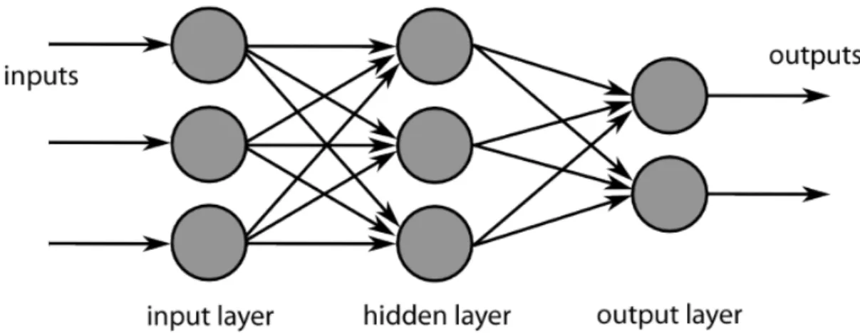
Neurons are organized as layers. Neurons in the same layer do not connect to each other. Neu-rons with no previous layers are calledinputs, and neurons with no next layers are calledoutputs. The layers between inputs and outputs are calledhidden layers. The number of hidden layers can be more than one. Figure 2.1 shows a neural networks with one hidden layer. When the number ofhidden layers is relatively large, for instance greater than eight, it is considered as a “deep” neural network [74]. Modern deep neural networks these days can have more than hundreds of layers [47]. Each connection between two neurons in neighbouring layers is assigned a weight

adjust-Figure 2.1: A neural network with one hidden layer

ment typically use gradient descent technique. The procedure of updating the weights according to different inputs is callednetwork training.

Gradient descent is a first-order numerical optimization method in finding the local optimal by calculating the gradient of the loss function and moving weights in the negative direction of the gradients with a specific step length. The step length is proportional to the absolute value of the gradient and this ratio is known aslearning rate. Back propagation (BP) algorithm [77] is the most important part in gradient descent as it is the key step in calculating the gradient. BP consists of four critical steps:

1. Feed-forward pass (inference): The linear combination and non-linear activation functions are evaluated layer by layer from input neuron to the output neuron. The final outputs from output neurons could be continuous value when the problem is regression or discrete values if the problem is a classification problem. This outputs could be right or wrong. It is decided by using a certainloss function.

2. BP on output layer: Firstly, an error value is calculated by this loss function. Next, the derivatives are calculated on loss function using this error value. At last, the derivatives are propagated back to the previous layer as gradients.

3. BP on hidden layers: The gradients are calculated iteratively following the fashion of previous step until it reaches the input layer.

2.2 Deep Learning and Neural Networks 23 4. Weight updates: Each weights are updated using the corresponding gradients at the same

place.

A cycle of above four steps is called a training iteration. Iterations continue until the BP algorithm converges (the gradients become sufficiently small).

Deep learning has been applied to a wide range of applications such as image recognition and natural language processing. Beyond image recognition, computer vision domain enjoys re-markable performance enhancement after using deep neural network to generate features auto-matically [74] instead of using human selected features. A bunch of advanced techniques, such as dropout [106], batch normalization [60], and residual [47], are developed recently. With these techniques adopted, the accuracy in image classification on deep neural networks over large dataset beats the accuracy of human beings [47] for the first time. Many vision based applications, e.g. self-driving vehicles [15] and medical treatments [135], largely benefited from the development of DNNs. Recurrent neural networks (RNNs), as a variant of DNNs, is different from previously described convolutional neural networks (CNNs). RNNs suits the sequential data best. They have the power to greatly improve the accuracy in speech recognition [49], natural language process-ing [23], and machine translation [8]. Another branch of the applications of DNNs is deep rein-forcement learning. This branch is extremely useful in robotic grasping [79] and game playing through self-learning [102].

2.2.2 Neural Network Architectures

We describe the neural network architectures used in the evaluation of our proposed C-LPT paradigm. These architectures include two types of neural networks, i.e., multi-layer perceptron (MLP) and convolutional neural network (CNN).

MLPMLP is constructed with a number of connected layers. Two neighbouring fully-connected layers connect to each other with the help of a non-linear layer in the middle. It is called fully-connected because each neuron in layericonnects all neurons in layer i+1and so on. Therefore, the computation in MLP is basically matrix or vector multiplication. LeNet-300-100 [78] is designed as a MLP with two hidden layers of size 300 neurons and LeNet-300-100 neurons,

Figure 2.2: LeNet-5 Architecture [78]

respectively.

CNNBeing different from MLP, CNN is not fully-connected. This is typically used in image processing. Because of the spatial locality of images, CNN shares weights in different space. And this weight sharing technique makes the model size much smaller compared to using fully-connected layers when the input image dimensions are the same. We evaluate with following four CNNs.

• LeNet-5[78] is a CNN with two convolutional layers and two fully-connected layers after them. This relatively simple network is used to recoginze hand written digits. The structure is shown in Figure 2.2.

• AlexNet [74] was proposed in 2012. It takes the advantage of strong computation power of GPUs and achieves a remarkable low error rate in image classification, top-1 error rate of 42.8% and top-5 error rate of 19.7% on ImageNet dataset. Before AlexNet, the features are normally manually selected. In comparison, AlexNet lets the CNN train these features on its own instead. The convolutional layers are of different kernel sizes. It starts from size 11×11 and reduces to 5×5 as the layer gets deeper, reaches3×3 at last. There are 5 convolutional layers and three fully-connected layers, and there are around 60 million parameters in total. Figure 2.3 shows the structure of AlexNet.

• VGG-16[105] After the appear of AlexNet, there is a rush in manufacturing deeper CNNs in the several following years. VGG-16 appeared in 2014. It has thirteen convolutional layers and three fully-connected layers with more than 130 million parameters in total. It significantly reduces the error rate even further, top-1 error rate of 21.5% and top-5 error rate

2.2 Deep Learning and Neural Networks 25

Figure 2.3: AlexNet Architecture [74]

Figure 2.4: VGG-16 Architecture [105]

of 11.3% using ImageNet dataset. The most different part from AlexNet is that VGG uses the same kernal size of3×3 throughout all convolutional layers. It demonstrates a high generalization capability in many applications. With the development of transfer learning, the pre-trained VGG-16 net using ImageNet has been widely used in areas of image clas-sification, object detection and image segmentation. Figure 2.4 shows the architecture of VGG-16.

• ResNet[47] ResNet is another milestone in model manufacturing. It was proposed in 2015, and introduces “bypass” layers to the convolutional parts. These “bypass” layers separate the CNN with several residual blocks. This design is motivated by the observation that the gradients tend to be too small to be able to pass from the output to the input as the number of layers goes higher. The proposal of residual blocks allow gradients to pass more easily from the end to the beginning. ResNet has 49 convolution layers and one fully-connected layer. Therefore it is known as ResNet-50 as well. It has around 26 million parameters to be trained. Each residual block aggregates the current feature map and feature map passes from previous residual block element-wisely. It achieves top-1 error rate of 23.9% and top-5

Figure 2.5: ResNet Architecture [47]

Figure 2.6: DeepSpeech Architecture, DeepSpeech 1 on the left [46] and DeepSpeech 2 on the right [2]

error rate of 7.1% on ImageNet. ResNet-50 makes a perfect balance between computational complexity and accuracy performance. Its structure is shown in Figure 2.5.

• DeepSpeech[2, 46] DeepSpeech 1 is a bidirectional recurrent neural network designed for speech recognition task, which has 8 million parameters in total, including five layers of neurons and one bi-directional recurrent layer. DeepSpeech 2 makes improvement on the first version and has a much bigger network in terms of the number of parameters. It has around 70 million parameters with seven bi-directional recurrent layer. The development of DeepSpeech model makes it become the default end-to-end training method for speech recognition instead of previous hybrid NN-HMM model. The illustration of DeepSpeech structure is shown in Figure 2.6.

2.3 Quantized Neural Network Training 27 There is a large number of studies that try to improve the computational performance of neural networks due to their popularity and importance. A branch of such studies tries to simplify the models while maintaining the accuracy because it is believed that these neural networks with millions of parameters have significant redundancy, which makes the models over-parameterized. Too much redundancy can lead to more computational effort and higher communication costs. Also when deploying them for applications, it is a waste of the memory. Generally speaking, there are two main streams in making networks more concise: pruning the weights and using lower precision (quantize weights to fewer bits). Because in this thesis we put more attention to training neural networks using lower precision, we restrict the scope of the related work to the second stream, quantized neural network training, and describe the existing work.

There have been several work proposing approaches to reduce the precision and bit width. Gong et al. [41] and Wu et al. [122] applied k-means scalar quantization to the parameter values. Vanhoucke et al. [117] explored a fixed-point implementation with 8-bit integer (vs 32-bit floating point) activations and showed that 8-bit quantization of the parameters can result in significant speed-up with minimal loss of accuracy. Abwer et al. [5] used L2 error minimization to quantize the neural networks. Hash function is used in work [20] to build HashedNets so that the bit width of parameters are reduced by grouping weights into hash tables. Hwang et al. [58] proposed an optimization method for neural network with ternary weights and 3-bit activation functions.

More aggressive approaches pushed the bit width even narrower. In the extreme case of 1-bit representation of each weight, we have existing work such as binary weight [24], or ternary weights [137]. Except from quantizing the weights only, work [94, 136] tried to quantize the acti-vation to a low precision as well. Matrix multiplication can be replaced by XNOR if both weights and activation are quantized. Another is to replace the matrix multiplication by shifts, which is even cheaper. This is realized by Miyashita et al. [88]. They adopted logarithmic quantization into the design of the model and experiments demonstrate its competitive performance.

The accuracy of such quantized networks do not show much accuracy loss using small models but the accuracy is significantly lowered when dealing with large CNNs such as GoogleNet. To address this issue, the work in [51] used second-order methods and proposed a proximal Newton algorithm with diagonal Hessian approximation that directly minimizes the loss with respect to the quantized weights. The work in [83] reduced the time on float point multiplication in the

training stage by stochastically binarizing weights and converting multiplications in the hidden state computation to sign changes.

Chapter 3

Real-time Hypergraph Partitioning for

Distributed Learning

1

3.1

Introduction

Among many applications, hypergraphs are used to represent the data records with rich structures and high-dimensional relationships. In these applications, the data records are represented by ver-tices, and the relationships among records are represented as hyperedges. When such applications involve huge amount of data, the size of the hypergraphs built can be very large. Minimizing the query cost on such hypergraphs is crucial for the applications. In this scenario, hypergraph parti-tioning helps to partition the query loads to several workers, which enables horizontal scaling of the large-scale hypergraphs.

Hypergraph partitioning requires a decomposition of a full hypergraph into multiple subsets such that the inter-dependency between sets is lower than the intra-dependency between the ele-ments in the same subset. This applies to a variety of applications in practice, in which one need to partition a set of items into disjoint components such that similar items are assigned to the same component in order to minimize the number of relationships between groups. This problem arises in the context of clustering of information objects such as documents, images and web-pages. For example, the goal may be to partition given collection of documents into sub-collections so that the maximum number of distinct topics in each sub-collection is minimized.

Partitioning hypergraphs in these applications require a clear trade-off between data locality and workload balance, as the intra-dependency and inter-dependency correspond to local and re-1_{Part of this chapter has been published in: Jiang, W., Qi, J., Yu, J., Huang, J., and Zhang, R. (2018). HyperX: A}

scalable hypergraph framework. IEEE Transactions on Knowledge and Data Engineering.

mote accesses to the data records, respectively. Minimizing the inter-dependenci