Distributed Tuning of Machine Learning Algorithms using MapReduce Clusters

(1)

Distributed Tuning of Machine Learning Algorithms using

MapReduce Clusters

Yasser Ganjisaffar

University of California, Irvine

Irvine, CA, USA

Thomas Debeauvais

Irvine, CA, USA

Sara Javanmardi

Irvine, CA, USA

Rich Caruana

Microsoft Research Redmond, WA 98052

Cristina Videira Lopes

Irvine, CA, USA

ABSTRACT

Obtaining the best accuracy in machine learning usually re-quires carefully tuning learning algorithm parameters for each problem. Parameter optimization is computationally challenging for learning methods with many hyperparame-ters. In this paper we show that MapReduce Clusters are particularly well suited for parallel parameter optimization. We use MapReduce to optimize regularization parameters for boosted trees and random forests on several text prob-lems: three retrieval ranking problems and a Wikipedia van-dalism problem. We show how model accuracy improves as a function of the percent of parameter space explored, that accuracy can be hurt by exploring parameter space too aggressively, and that there can be signiﬁcant interaction between parameters that appear to be independent. Our results suggest that MapReduce is a two-edged sword: it makes parameter optimization feasible on a massive scale that would have been unimaginable just a few years ago, but also creates a new opportunity for overﬁtting that can reduce accuracy and lead to inferior learning parameters.

Categories and Subject Descriptors

H.4.m [Information Systems]: Miscellaneous—Machine Learning

General Terms

Algorithms, Experimentation

Keywords

Machine learning, Tuning, MapReduce, Hyper–parameter, Optimization

Permission to make digital or hard copies of all or part of this work for personal or classroom use is granted without fee provided that copies are not made or distributed for profit or commercial advantage and that copies bear this notice and the full citation on the first page. To copy otherwise, to republish, to post on servers or to redistribute to lists, requires prior specific permission and/or a fee.

1. INTRODUCTION

The ultimate goal of machine learning is to automatically build models from data without requiring tedious and time consuming human involvement. This goal has not yet been achieved. One of the difficulties is that learning algorithms require parameter tuning in order to adapt them to the par-ticulars of a training set [14, 7]. The number of nearest neighbors in KNN or the step size in stochastic gradient descent are examples of these parameters. Researchers are expected to maximize the performance of their algorithm by optimizing over parameter values. There is little literature in the machine learning community about how to optimize hyperparameters efficiently and without overfitting. As just one example, support vector machine classification requires an initial learning phase in which the training data are used to adjust the classification parameters. There are many pa-pers about SVM algorithms and kernel methods, but few of them address the parameter tuning phase of learning which is critical to achieve high quality results. Because of the diffi-culty of tuning parameters optimally, sometimes researchers use complex learning algorithms before experimenting ade-quately with simpler alternatives with better tuned parame-ters [14], and reported results are more difficult to reproduce because of the influence of parameter settings [16].

Despite decades of research into global optimization and the publishing of several parameter optimization algorithms [13, 18, 5], it seems that most machine learning researchers still prefer to carry out this optimization by hand or by grid search [12]. Grid search uses a predefined set of values for each parameter and determines which combination of these values yields the best results. Grid search is computation-ally expensive and takes substantial time when performed on a single machine. However, given the independence of these experiments, they can easily be performed in paral-lel. Thus parallel grid search is easy and scalable. With the increasing availability of inexpensive cloud computing envi-ronments grid search parameter tuning tuning on large data sets has become more practical. Cloud computing makes massive parameter exploration so easy that a new problem arises: the final accuracy of the model on test data can be reduced by running too many experiments and overfitting to the validation data.

In this work, we use the MapReduce framework [6] to eﬃ-ciently perform parallel grid search for exploring thousands of combinations of parameter values. We propose a general

(2)

approach that can be used for tuning parameters in diﬀerent machine learning algorithms. The approach is easiest to un-derstand when each tuning task (evaluating the performance of the algorithm for a single combination of parameter val-ues) can be handled by a single node in the cluster, but also works when multiple processors are needed for each train-ing run. For strain-ingle node traintrain-ing runs, the node loads the training and validation data from the distributed ﬁle system of the cluster and learns a model on the training data and reports the validation data. The next section describes the details of this method. The main advantage of the MapRe-duce framework for parameter tuning is that it can be used for very large optimizations at low cost. In section 2, we de-scribe how easy it is to perform massive parallel grid search on MapReduce clusters. The MapReduce framework allows us to focus on the learning task and not worry about paral-lelization issues such as communications between processes, fault tolerance and etc.

We report the results of our experiments on tuning the pa-rameters of two machine learning algorithms that are used in two different kinds of tasks. The first learns ranking mod-els for information retrieval in search engines. The goal is to train an accurate model that given a feature vector which is extracted from a query–document pair, assigns a score to the document which is then used for ordering documents based on their relevance to the query. The second kind of task is a binary classification task that uses Random Forests [2] to detect vandalistic edits in Wikipedia. Wikipedia contribu-tors can edit pages to add, update or remove content. An edit is considered vandalistic if valuable content is removed or if erroneous or spam content is added.

In the ﬁrst part of the paper we describe how to use MapReduce for parameter optimization. The second part of the paper describes the application of MapReduce to opti-mize the parameters of boosted tree and random forest mod-els on the four text problems. The third part of the paper discusses lessons learned from performing massive parame-ter optimization on these problems. We show the increase in accuracy that results from large-scale parameter optimiza-tion, the loss in accuracy that can result from searching pa-rameter space too thoroughly, and how massive papa-rameter optimization uncovers interactions between parameters that one might not expect.

2. MAPREDUCE FOR PARAMETER

TUN-ING

We use cross–fold validation and evaluate the performance of the algorithm for the same set of parameters on differ-ent folds of the data and use the average over these folds for deciding which combination of parameters should be used. Some learning algorithms involve random processes that may result in significantly different results for different runs of the algorithm with different random seeds. In these cases, we repeat the process several times for different ran-dom seeds and use the average results for picking the best parameter values. In summary, if there areN combinations of parameters that need to be evaluated, we performK×S experiments for each combination, whereK is the number of data folds andSis the number of different random seeds that we use. Using this approach we would be able to report the average and variance of our evaluation metrics for each of theNcombinations. However, this setup requires a total

of N ×K×S experiments that may take a long time on relatively large data sets.

Given that all the experiments are independent from each other, a cluster of machines can be used for performing these experiments in parallel and then aggregating results. MapReduce clusters are particularly well suited for this pur-pose. The master node can initiateMapa map task for each of the N×K×S tasks. Each map task uses the param-eter values that are assigned to it to learn a model on the training data that is assigned to it and then measures the performance of the model on the corresponding validation data. Algorithm shows the description of a Map task.

The MapReduce framework automatically combines the K×S results which are computed for the same set of pa-rameter values for diﬀerent folds of the data and diﬀerent random seeds. These results are then passed to reducer tasks. Reducers just compute the mean and standard de-viation of the list of measurements and emit them in their output. Algorithm shows the description of a Reducer task.

Algorithm 1:Map: (Θ, k, s) → (Θ, ρ)

input :Θ, list of parameter values

input :k, fold number

input :s, random seed

• Train learning modelM on training data of foldk using the list of parameter valuesΘ and the random seeds

• Computeρ: the performance of modelM on validation data of foldk

output: (Θ, ρ)

Algorithm 2:Reduce: (Θ,(ρ1, . . . ρm)) → (Θ,ρ, σ¯ )

input :Θ, parameter values

input : (ρ1, . . . ρm), performance values of diﬀerent

folds and random seeds computed for parameter valuesΘ by mapper tasks Compute average (¯ρ) and standard deviation (σ) of input performance values.

output: (Θ,ρ, σ¯ )

In the next two sections, we show how we used this archi-tecture for two diﬀerent learning tasks.

3. TASK 1: LEARNING TO RANK

We use LambdaMART [20] for learning a ranking model for task 1. LambdaMART is a ranking algorithm that uses Gradient boosting [9] to optimize a ranking cost function. Gradient boosting produces an ensemble of weak models (typically regression trees) that together form a strong model. The ensemble is built in a stage-wise process by performing gradient descent in function space. The ﬁnal model maps an input feature vectorx∈Rdto a scoreF(x)∈R:

Fm(x) =Fm−1(x) +γmhm(x)

where each hi is a function modeled by a single regression

(3)

regression tree. Both thehi and theγi are learned during

training. A given treehi maps a given feature vectorxto

a real value by passing x down the tree, where the path (left or right) at a given node is determined by the value of a particular feature in the feature vector and the output is a ﬁxed value associated with the leaf that is reached by following the path.

Gradient boosting usually requires regularization to avoid overfitting. Different kinds of regularization techniques can be used to reduce overfitting in boosted trees. One common regularization parameter is the number of trees in the model, M. Increasing M reduces the error on training set, but setting it too high often leads to overfitting. An optimal value ofM often is selected by monitoring prediction error on a separate validation data set.

Another regularization approach is to control the com-plexity of the individual trees via a number of user-chosen parameters. For example,Max Number of Leaves per tree

limits the size of individual trees thus preventing them from overﬁtting to the training data. Another user–set parameter for controlling tree size is the minimum number of observa-tions allowed in leaves. This parameter is used in the tree building process by ignoring splits that lead to nodes con-taining fewer than this number of training set observations. This prevents adding leaves that contain statistically small samples of training data.

Another important regularization technique is shrinkage which modiﬁes the boosting update rule as follows:

Fm(x) =Fm−1(x) +ηγmhm(x), 0< η≤1,

where parameterηis called thelearning rate. Small learn-ing rates can dramatically improve a model’s generalization ability over gradient boosting without shrinkage (η = 1), however they result in slower convergence and more boost-ing iterations and therefore larger models.

In [8], Friedman proposed a modification of the gradient boosting algorithm which was motivated by Breiman’s bag-ging method. He proposed that at each iteration of the al-gorithm, a base learner should be fit on a sub-sample of the training set drawn at random without replacement. Fried-man observed a substantial improvement in gradient boost-ing’s accuracy with this modification. Sub-sample size is some constant fractionsof the size of the training set. When s = 1, the algorithm is deterministic. Smaller values of s introduce randomness into the algorithm and help prevent overfitting, acting as a kind of regularization. The algorithm also becomes faster, because regression trees have to be fit to smaller data sets at each iteration.

Also similar to Random Forests [2], more randomness can be introduced by sampling features that are available to the algorithm on each tree split. On each split, the algorithm selects the best feature from a random subset of features instead of the best overall feature.

In our experiments, we add both observation sub-sampling and feature sampling as two new parameters that need to be tuned for the LambdaMART algorithm. These parameters can take values between 0 and 1, where 1 means no sam-pling and values less than 1 introduce samsam-pling randomness. Taken together, all of these parameters present a large hy-perparameter search space over which to optimize learning performance.

3.1 Data sets

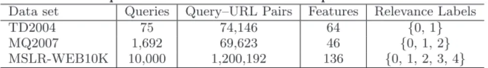
For our experiments we work with three public data sets: TD2004 and MQ2007 from LETOR data sets [17] and the recently published MSLR-WEB10K data set from Microsoft Research [1]. Table 1 summarizes the properties of these data sets. The three data sets contain diﬀerent number of queries and have diverse properties. Therefore we expect diﬀerent parameter values after tuning the same models on each of them.

3.2 Evaluation Metric

For model comparison we use NDCG@k which is a popular information retrieval metric [11]. NDCG@k is a measure for evaluating top k positions of a ranked list using multiple levels of relevance judgment. It is deﬁned as follows,

NDCG@k=N−1 k j=1 2rj₋₁ log₂(1 +j),

whereN−1is a normalization factor chosen so that a per-fect ordering of the results will receive the score of one and rjdenotes the relevance level of the document ranked at the

j-th position.

3.3 Parameter Tuning

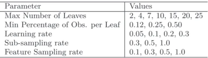
We use grid search to test 1,008 diﬀerent combinations of parameters on the smaller data sets and 162 combinations on the larger data set. Table 2 shows the values we tried for each of the parameters. Since MSLR-WEB10K contains more features for each query–url pair, we need more com-plex trees (trees with more leaves) on this data set. We do not directly control the best number of trees for the Lamb-daMART models via a user–set parameter. Instead, as iter-ations of boosting continue, the prediction accuracy of the model is checked on a separate validation set. Boosting con-tinues until there has been no improvement in accuracy for 250 iterations. The algorithm then returns the number of iterations that yielded maximum accuracy on the validation set.

Each combination of parameters is tested on 5 folds of each data set. On each fold we use 3 diﬀerent random seeds to get more accurate results. This requires 1,008×5×3 = 15,120 experiments on each of the smaller data sets and 162×5×3 = 2,430 experiments on MSLR-WEB10K. We used a MapReduce cluster of 40 nodes for these experiments. It takes only 8 hours to run all of these experiments on this cluster.

Table 3 shows the best configurations based on Validation NDCG@3 on each data set. The best performing configura-tions on all three data sets use feature sampling. The smaller data sets also get better results by sub-sampling of training queries on each iteration. We conjecture that sub-sampling queries helps when the training data is small because it helps avoid overfitting by not allowing trees to see all queries on each iteration of boosting. This adds diversity to the indi-vidual trees which is then reduced when boosting averages tree predictions. With very large data sets this is less criti-cal because individual trees cannot themselves significantly overfit a large data set when tree size is limited.

(4)

Table 1: Properties of data sets used for experiments in Task 1

Data set Queries Query–URL Pairs Features Relevance Labels

TD2004 75 74,146 64 {0, 1}

MQ2007 1,692 69,623 46 {0, 1, 2}

MSLR-WEB10K 10,000 1,200,192 136 {0, 1, 2, 3, 4}

Table 3: Best three combinations of parameters found after parameter tuning for the Ranking Tasks

Validation NDCG@3 Max Leaves Min Obs. Per Leaf Learning Rate Sub–sampling Feature Sampling

0.5113 20 0.25 0.1 0.5 0.1

0.5105 10 0.50 0.05 0.3 0.1

0.5061 10 0.12 0.05 0.5 0.3

(a) TD2004 data set

0.5647 7 0.25 0.05 0.3 0.3

0.5643 4 0.25 0.1 1.0 0.1

0.5643 10 0.25 0.05 0.5 0.3

(b) MQ2007 data set

0.4873 40 0.25 0.1 1.0 0.5

0.4872 70 0.50 0.05 1.0 0.3

0.4870 40 0.25 0.05 1.0 0.5

(c) MSLR-WEB10K data set

4. TASK 2: DETECTING VANDALISTIC

ED-ITS IN WIKIPEDIA

The goal of this task is to detect vandalistic edits in Wikipedia articles. Deletion of valuable content or insertion of obvi-ously erroneous content or spam are examples of vandalism in Wikipedia.

We consider vandalism detection as a binary classification problem. We use the PAN 2010 corpus [15] for training the classifier and evaluating its performance. This data set is comprised of 32,452 edits on 28,468 different articles. It was annotated by 753 annotators recruited from Amazon’s Mechanical Turk, who cast more than 190,000 votes so that each edit has been reviewed by at least three of them. The corpus is split into a training set of 15,000 edits and a test set of 18,000 edits. To learn and predict vandalistic edits we extract 66 features for each sample in this data set.

The ratio of vandalistic edits in this data set is 7.4%. Therefore we have about 13 times more negative samples than positive (vandalistic) samples. Hence, we need to use learning algorithms which are robust to imbalanced data, or to transform the data to make it less imbalanced. Random forests [2] are known to be reasonably robust to imbalanced datasets and therefore we used this algorithm for our clas-siﬁcation task. For evaluation, we use AUC which has been reported to be a robust metric for imbalance problems [19].

4.1 Algorithms

Several diﬀerent methods have been proposed to further

improve the eﬀectiveness of random forests on imbalanced data. Oversampling the minority class, undersampling the majority class, or a combination of these have been used for this purpose. We useN+to represent the number of vandal-istic samples andN−_{the number of legitimate samples. In}

each of the 3 folds of the PAN train set we haveN+≈600 and N− ≈9400. We use N_b+ and N_b− for referring to the number of positives and negatives in a bag.

Chenet al. [4] introduced Balanced Random Forests (BRF)

in which they undersample majority on each bag, while all of the minority cases are included in all the bags:

N+

b =Nb−=N+

Based on Chen’s method, Hidoet al. [10] proposed a Roughly Balanced Random Forest (RBRF) which is similar to BRF with the exception that the number of negative samples in a roughly balanced bagN_b−is drawn from a negative binomial distribution centered onN+ instead of exactlyN+.

Bags can also be forced to become balanced by oversam-pling the minority samples. In our dataset, we would need to oversample the minority by 1300% to reach balance. Again, bags could be “roughly” balanced by using the above ap-proach. In our experiments, to increase diversity of the bags, we pick both minority and majority cases with replacement. Mixing oversampling of the majority and undersampling of the minority can also result in balanced bags. In our data set, this would be achieved by undersampling the majority

(5)

Table 2: Values used in grid search for parameter tuning of the Ranking Task

Parameter Values

Max Number of Leaves 2, 4, 7, 10, 15, 20, 25

Min Percentage of Obs. per Leaf 0.12, 0.25, 0.50

Learning rate 0.05, 0.1, 0.2, 0.3

Sub-sampling rate 0.3, 0.5, 1.0

Feature Sampling rate 0.1, 0.3, 0.5, 1.0

(a) TD2004 and MQ2007 data sets

Parameter Values

Max Number of Leaves 10, 40, 70

Min Percentage of Obs. per Leaf 0.12, 0.25, 0.50

Learning rate 0.05, 0.1, 0.2

Sub-sampling rate 0.5, 1.0

Feature Sampling rate 0.3, 0.5, 1.0

(b) MSLR-WEB10K data set

by approximately 50% and oversampling the minority by approximately 700%.

Oversampling the minority can also be achieved by gener-ating synthetic data. We used SMOTE [3] for this purpose. SMOTE randomly picks a positive sample pand creates a synthetic positive samplepbetweenpand one of the near-est neighbors of p. SMOTE has two hyper parameters: k, the number of nearest neighbors to look at, andr, the over-sampling rate of minority cases (e.g.,r= 100% doubles the minority size). The combination of various under and over-sampling parameters with the SMOTE parameters yiels a large conﬁguration space.

4.2 Parameter tuning

To train a random forest classiﬁer, we need to tune two free parameters: the number of trees in the model and the the number of features selected to split each node. Our experiments show that on this problem classiﬁcation perfor-mance is sensitive to the number of trees but less sensitive to the number of features in each split. This result is con-sistent with Breiman’s observation [2] on the insensitivity of random forests to the number of features selected in each split.

To tune the number of trees, we partition the train set into three folds and use 3–fold cross validation. To find the mini-mum number of trees consistent with excellent performance, we need to sweep a large range of model sizes. Hence, we need to design an efficient process for this purpose. For each fold, we create a pool ofN= 10,000 trees, each trained on a random sample of the training data in that fold. Then we use this pool for creating random forests of different sizes. For example, to create a random forest with 20 trees, we randomly select 20 trees from this pool ofN trees. How-ever, since this random selection can be done inC(N,20) different ways, each combination may result in a different AUC. We repeat the random selection of treesr= 20 times and we report the mean and variance of theF×r results (whereF is the number of folds).

The advantage of this approach is that we can calculate

Table 4: Values used in grid search for parameter tuning of Task 2

Parameter Values

Oversampling rate none, 700%, 1300% Undersampling rate none, 50%, 8%

Balance type exact, rough

(a) Bagging strategies

Parameter Values

Nearest neighbors 1, 3, 5, 7, 9, 11, 13, 19, 25, 31, 37 Oversampling rate none, 100%, 200%, ... , 1300%

(b) SMOTE conﬁgurations

the mean and variance of AUC very eﬃciently for forests with diﬀerent sizes without the need to train a huge number of trees independently. Otherwise, to report the mean and variance of AUC for random forests of size k= 1 to T, we would need to trainr+2×r+3×r+...+T×r=r∗T(T+1)/2 trees for each fold, which is 40 million trees in our case. Using this approach we only need to trainN trees per fold which is 30 thousand trees.

Table 4 shows the values that we tried for each of the pa-rameters for both oversampling/undersampling and SMOTE. The rates for oversampling and undersampling are picked based on the strategies mentioned in the previous section. For the SMOTE experiments, we tried 11 values for nearest neighbors and 14 values for oversampling rate.

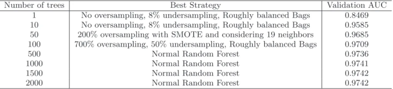
We used a MapReduce cluster of 40 nodes for these exper-iments. It takes about 75 minutes to run these experiments once on this cluster. Table 5 shows the best strategy in terms of validation AUC as we vary the number of trees in the forest. For very small forests, undersampling the ma-jority works best. For medium size forests, oversampling the minority class works best; and for large forests, normal random forest (no oversampling and no undersampling) is best. We had not expected that the best method to use to handle the imbalanced data problem would vary so strongly with the number of trees in the random forest. In particular, we had not expected that undersampling the majority class with no oversampling of the minority class would be best for small random forests, but that as the forests become larger oversampling of the minority class would become beneﬁcial. We also did not expect that the best way to handle class imbalance would be to do nothing as the number of trees in the forest grew large. The best on this problem results from using a large (≥500) number of trees (expected) and taking no steps to correct class imbalance (unexpected).

5. DISCUSSION

The MapReduce clusters allowed us to tune model pa-rameters very thoroughly. It would be interesting to know whether we really needed that many experiments to achieve high accuracy, and if it is possible to perform too many ex-periments.

We use the results of our parameter tuning experiments to study the eﬀect of number of experiments on

(6)

improve-Table 5: Best combinations of parameters found after parameter tuning for Task 2. The best strategy in terms of AUC depends on the number of trees in the forest. For very small forests, undersampling the majority works best. For medium size forests, oversampling the minority works best; and for large forests, normal random forest (no oversampling and no undersampling) is the winner

Number of trees Best Strategy Validation AUC

1 No oversampling, 8% undersampling, Roughly balanced Bags 0.8469

10 No oversampling, 8% undersampling, Roughly balanced Bags 0.9585

50 200% oversampling with SMOTE and considering 19 neighbors 0.9685

100 700% oversampling, 50% undersampling, Roughly balanced Bags 0.9709

500 Normal Random Forest 0.9736

ment in the evaluation metrics. For each dataset, we create a pool of configurations that we evaluated during parame-ter tuning experiments. Then we randomly select different numbers of these configurations. On each random selection, we pick the configuration with best validation performance and then record validation and test performance for that configuration. To get more accurate results, we repeat this random process 10,000 times and report average numbers.

Figure 1 shows the results for the three ranking Tasks. As expected, for all three data sets, validation NDCG im-proves monotonically as we perform more experiments. On MSLR-WEB10K, the largest data set, there is less discrep-ancy between validation and test scores. The discrepdiscrep-ancy between validation and test is largest on TD2004, the small-est data set, because the validation sets which are held aside form the training data must also be small.

On TD2004, the data set with the smallest validation sets, accuracy on the test set peaks after only about 100 param-eter configurations, and then slowly drops. Accuracy on the validation set is still rising significantly at 100 itera-tions, suggesting that hyperparameter optimization is over-fitting to the validation sets. A similar effect is observed on MQ2007, but overfitting does not begin on this problem until about 400 parameter configurations have been tried. And on MSLR-WEB10K, we again observe overfitting to the validation sets after fewer than 25 configurations have been tested.

Figure 2 shows the effect of validation set size on the over-fitting of the hyperparameters on the MQ2007 problem. The leftmost graph is for validation sets that contain only 10% of the number of points used for this problem in Figure 1; the middle graph is for 50%, and the rightmost graph is for 100%. When the validation set is very small (left graph), the gap between validation and test set performance is very large, overfitting to the validation set occurs after only a few dozen hyperparameter configurations have been tested, and the loss in accuracy on the test set is considerable if the full configuration space is explored. On problems like this, exploiting the full power of a MapReduce Cluster for parameter optimization can significantly hurt generalization instead of helping it.

As the size of the validation set grows to 50% of maxi-mum size, the discrepancy between the validation and test set performance drops significantly, overfitting to the vali-dation set does not begin until 100 configurations have been explored and is modest at first, and the loss in generaliza-tion that results from exploring the full configurageneraliza-tion space

is less. As the validation set becomes larger (right graph), the discrepancy between validation and test is further re-duced, overfitting to the validation set does not occur until 400 or more parameter configurations have been tested, and the drop in generalization accuracy on the test set as more of the parameter space is explored is small. Surprisingly, there is still a drop in accuracy of a few tenths of a point if the full space is explored even with full-size validation sets from a 5-fold cross-validation averaged across the five folds on a problem with 10k training examples, suggesting that care must still be exercised when peak accuracy is required. When there is randomness in the algorithm and the vali-dation sets are not infinite, as more parameter combinations are tried search begins to find parameter combinations that look better on the validation set because of this random-ness. If one is not careful, the computational power pro-vided by MapReduce Clusters is so great that it is possible to overdo parameter tuning and find parameter combina-tions that work not better than the hyperparameters that would have been found by less thorough search. One way to avoid overfitting at the hyperparameter learning stage is to use a 2nd held-out validation set to detect when parameter tuning begins to overfit and early-stop the parameter opti-mization. Holding out a 2nd validation set will reduce the size of the primary hyperparameter tuning validation sets, making overfitting more likely. But as we have seen, even large cross-validated validation sets do not completely pro-tect from overfitting when hyperparameter optimization is exhaustive, so care must be exercised to prevent hyperpa-rameter optimization from becoming counterproductive.

6. CONCLUSION

MapReduce clusters provide a remarkably convenient and aﬀordable resource for tuning machine learning hyperparam-eters. Using these resources one can quickly run massive pa-rameter tuning experiments that would have been infeasible just a few years ago. In this paper we show how to map parameter optimization experiments to the MapReduce en-vironment. We then demonstrate the kinds of results that can be obtained with this framework by applying it to four text learning problems. Using the framework we were able to uncover interactions between hyperparameters that we had not expected. For example, the best method for deal-ing with imbalanced classes in the classiﬁcation problem de-pends on how many trees will be included in the random forest model. When there will be relatively few trees in the forest (less than X) it is important to reduce class imbalance

(7)

0 200 400 600 800 1000 0.40 0.42 0.44 0.46 0.48 0.50 TD2004 data set

Number of tuning experiments

NDCG@3 ●●●●●●●●●●●● ●●●●●●●●●●●●●●●●●●●●●●●●● ●●●●●●●●●●●●●●●●●●●●●●●●●●●●●●●●●●●●●●●●●●●●●●●●●●●●●●●●●●●●●●● ● Validation Test 0 200 400 600 800 1000 0.552 0.554 0.556 0.558 0.560 0.562 0.564 MQ2007 data set

NDCG@3 ● ● ●● ●●●●●●●● ●●●●●●●●●●● ●● ●●●●●●●●●●●● ●●●●●●●●●●●●●●●●●●●●●●●●● ●●●●●●●●●●● ●● ●●●●●●●●●●●●●●●●●●●●●●●●● ● Validation Test 0 50 100 150 0.474 0.476 0.478 0.480 0.482 0.484 0.486

MSLR−WEB10K data set

NDCG@3 ● ● ● ●●● ●● ● ●● ● ●● ●● ● ●● ● ●● ●● ● ●● ●● ● ●● ● ●● ●● ● ●●● ●● ●● ● ●● ●● ● ●● ● ●● ●●_{● ●● ● ●● ●● ● ●● ● ●●} ●● ● ●● ●● ● ●●● ●● ●● ● ●● ● ●_{● ●● ● ●● ●●} ● Validation Test

Figure 1: As more combinations of parameters are tested during parameter tuning of LambdaMART, NDCG@3 improves on the validation sets, but the test set curves show overﬁtting of the hyperparameters eventually occurs. 0 200 400 600 800 1000 0.53 0.54 0.55 0.56 0.57 0.58 0.59

10% of the Validation set

NDCG@3 ● ● ●● ●●_●●● ●●●●●●●●●_{●●●●●●●●●●●} ●●●●●●●●●● ●●●●●●●●●●●●●●●●●●● ●●●● ●●●●●●●●●●●●●●●●●_{●●●●●●●●●●} ●●●●●●●●●●● ● Validation Test 0 200 400 600 800 1000 0.53 0.54 0.55 0.56 0.57 0.58 0.59

NDCG@3 ●●●●●●●●●●●● ●●●●●●●●●●●●●●●●●●●●●●●●●●●●●●●●●●●●●● ●●●●●●●●●●●_{● ●●●●●●●●●●●●●●●●} ●●●●●●●●●●●●●●●●●●●●●● ● Validation Test 0 200 400 600 800 1000 0.53 0.54 0.55 0.56 0.57 0.58 0.59

NDCG@3

●●●●●●●●●●●● ●●●●●●●●●●●●● ●●●●●●●●●●●● ●●●●●●●●●●●●● ●●●●●●●●●●●● ●●●●●●●●●●●●● ●●●●●●●●●●●●●●●●●●●●●●●●●

●

Validation Test

Figure 2: The eﬀect of validation set size on hyperparameter overﬁtting on the MQ2007 problem.

by over sampling the rare class, under sampling the majority class, or by using a method such as SMOTE to induce new rare class samples. But when the random forest grows large and contains 500 or more trees, the best results are obtained by not modifying the natural statistics in the raw data. An-other surprising result is that even when performing cross– validation using large validation sets, MapReduce makes it easy to explore hyperparameter space too thoroughly and overfit to the validation data. Experiments suggest that the risk is overwhelming with small validations sets, and that some risk of overfitting remains even when validation sets grow large. While we expected this result for small vali-dation sets, we had not expected the effect to remain with larger validation sets. We conclude that while MapReduce clusters provide an incredibly convenient resource for ma-chine learning hyperparameter optimization, one must pro-ceed with caution or risk selecting parameters that are as inferior as those that would have been found when the pa-rameter space could not have been explored as thoroughly.

Acknowledgments

Authors would like to thank Amazon for a research grant that allowed us to use their MapReduce cluster. This work has been also partially supported by NSF grant OCI-074806.

7. REFERENCES

[1] Microsoft learning to rank datasets.

http://research.microsoft.com/en-us/projects/mslr/. [2] L. Breiman. Random forests.Machine Learning,

45:5–32, 2001. 10.1023/A:1010933404324.

[3] N. V. Chawla, K. W. Bowyer, L. O. Hall, and W. P. Kegelmeyer. Smote: synthetic minority over-sampling technique.Journal of Artiﬁcial Intelligence Research, 16:321–357, June 2002.

[4] B. Chen, Liaw. Using random forest to learn imbalanced data. Technical report, Stanford, 2004. [5] I. Czogiel, K. Luebke, and C. Weihs. Response surface

methodology for optimizing hyper parameters. Technical report, Universitat Dortmund Fachbereich Statistik, 2005.

[6] J. Dean and S. Ghemawat. Mapreduce: simpliﬁed data processing on large clusters.Communications of ACM, 51:107–113, January 2008.

[7] T. Eitrich and B. Lang. Eﬃcient optimization of support vector machine learning parameters for unbalanced datasets.Journal of Computational and

Applied Mathematics, 196:425–436, November 2006.

[8] J. H. Friedman. Stochastic gradient boosting. Technical report, Technical report, Dept. Statistics, Stanford Univ., 1999.

(8)

[9] J. H. Friedman. Greedy function approximation: A gradient boosting machine.Annals of Statistics, 29:1189–1232, 2000.

[10] S. Hido and H. Kashima. Roughly balanced bagging for imbalanced data. InSIAM Data Mining, pages 143–152, 2008.

[11] K. Järvelin and J. Kekäläinen. IR evaluation methods for retrieving highly relevant documents. InSIGIR ’00: Proceedings of the 23rd annual international ACM SIGIR conference on Research and development

in information retrieval, pages 41–48, New York, NY,

USA, 2000. ACM.

[12] H. Larochelle, D. Erhan, A. Courville, J. Bergstra, and Y. Bengio. An empirical evaluation of deep architectures on problems with many factors of variation. InProceedings of the 24th international

conference on Machine learning, ICML ’07, pages

473–480, New York, NY, USA, 2007. ACM. [13] A. Nareyek. Choosing search heuristics by

non-stationary reinforcement learning.Applied

Optimization, 86:523–544, 2003.

[14] M. Postema, T. Menzies, and X. Wu. A decision support tool for tuning parameters in a machine learning algorithm. InPACES/SPICIS’97 Proceedings, pages 227–235, 1997.

[15] M. Potthast, A. Barr´on-Cede˜no, A. Eiselt, B. Stein, and P. Rosso. Overview of the 2nd international competition on plagiarism detection. InProceedings of the CLEF’10 Workshop on Uncovering Plagiarism,

Authorship and Social Software Misuse, 2010.

[16] F. Poulet. Multi-way Distributed SVM algorithms. In

Parallel and Distributed computing for Machine Learning. In conjunction with the 14th European Conference on Machine Learning (ECML’03) and 7th European Conference on Principles and Practice of

Knowledge Discovery in Databases (PKDD’03),

Cavtat-Dubrovnik, Croatia, September 2003. [17] T. Qin, T.-Y. Liu, J. Xu, and H. Li. LETOR: A

benchmark collection for research on learning to rank for information retrieval.Information Retrieval, 13:346–374, 2010. 10.1007/s10791-009-9123-y. [18] C. C. Ski´scim and B. L. Golden. Optimization by

simulated annealing: A preliminary computational study for the tsp. InProceedings of the 15th conference

on Winter Simulation - Volume 2, WSC ’83, pages

523–535, Piscataway, NJ, USA, 1983. IEEE Press. [19] G. M. Weiss. Mining with rarity: a unifying

framework.SIGKDD Explor. Newsl., 6:7–19, June 2004.

[20] Q. Wu, C. Burges, K. Svore, and J. Gao. Ranking, boosting and model adaptation. Technical report, Microsoft Technical Report MSR-TR-2008-109, 2008.

Distributed Tuning of Machine Learning Algorithms using MapReduce Clusters