Volume 17 | Issue 1 Article 4
2018
The Transmuted Exponentiated Additive Weibull
Distribution: Properties and Applications
Zohdy M. Nofal
Benha University, Egypt, [email protected]
Ahmed Z. Afify
Benha University, Egypt, [email protected]
Haitham M. Yousof
Benha University, Egypt, [email protected]
Daniele Cristina Tita Granzotto
Universidade Estadual de Maringá, PR, Brazil, [email protected]
Francisco Louzada
Universidade de São Paulo, SP, Brazil, [email protected]
Follow this and additional works at:https://digitalcommons.wayne.edu/jmasm
Part of theApplied Statistics Commons,Social and Behavioral Sciences Commons, and the
Statistical Theory Commons
Recommended Citation
Nofal, Z. M., Afify, A. Z., Yousof, H. M., Granzotto, D. C. T., & Louzada, F. (2018). The Transmuted Exponentiated Additive Weibull Distribution: Properties and Applications. Journal of Modern Applied Statistical Methods, 17(1), eP2526. doi: 10.22237/jmasm/ 1525133340
doi: 10.22237/jmasm/1525133340 | Accepted: April 9, 2017; Published: June 7, 2018. Correspondence: Daniele Cristina Tita Granzotto, [email protected]
The Transmuted Exponentiated Additive
Weibull Distribution: Properties and
Applications
Zohdy M. Nofal Benha University Benha, Egypt Ahmed Z. Afify Benha University Benha, Egypt Haitham M. Yousof Benha University Benha, Egypt Daniele C. T. Granzotto Universidade Estadual de Maringá Maringá, PR, BrazilFrancisco Louzada Universidade de São Paulo São Paulo, SP, Brazil
A new generalization of the transmuted additive Weibull distribution is proposed by using the quadratic rank transmutation map, the so-called transmuted exponentiated additive Weibull distribution. It retains the characteristics of a good model. It is more flexible, being able to analyze more complex data; it includes twenty-seven sub-models as special cases and it is interpretable. Several mathematical properties of the new distribution as closed forms for ordinary and incomplete moments, quantiles, and moment generating function are presented, as well as the MLEs. The usefulness of the model is illustrated by using two real data sets.
Keywords: Exponentiated additive Weibull distribution, transmutation map, moments, reliability analysis
Introduction
Focusing on the most popular positive probability distribution, the Weibull distribution, a new generalization is introduced, which is the transmuted exponentiated additive Weibull (TEAW). The Weibull model was proposed in 1951, being widely used in reliability analyses and in several different fields with different applications, see for example Lai, Xie, and Murthy (2003). Although it is widely used, a negative point of the distribution is the limited shape of its hazard function that can only be monotonically increase, decrease, or remain constant. Generally, practical problems require a wider range of possibilities in the medium
risk for example, when the lifetime data present a bathtub shaped hazard function, such as human mortality and machine life cycles.
Aiming at a more flexible Weibull distribution, researchers developed various extensions and modified forms of the Weibull distribution with different numbers of parameters (e.g., Lai, Xie, & Murthy, 2001; Nadarajah, 2009). Xie and Lai (1995) proposed a four-parameter additive Weibull (AW) distribution as a competitive model. In this paper we introduce the TEAW distribution which extends recent developments on the additive Weibull such as the transmuted additive Weibull introduced by Elbatal and Aryal (2013), transmuted exponentiated modified Weibull introduced by Eltehiwy and Ashour (2013), transmuted modified Weibull introduced by Khan & King (2013), modified Weibull introduced by Sarhan and Zaindin (2009), Marshall-Olkin additive Weibull proposed by Afify, Cordeiro, Yousof, Saboor, and Ortega (in press), and additive Weibull introduced by Xie and Lai (1995), among others.
Let X be a random variable distributed as an AW distribution; then its cumulative distribution function (cdf) is given by
(
)
F x; , , , = −1 e−x−x, x0 (1) where α, β, γ, θ > 0 with 0 < θ < β (or 0 < β < θ); θ and β are shape parameters and α and γ are scale parameters. The corresponding probability density function (pdf) of (1) is
(
)
(
1 1)
f x; , , , = x− +x− e−x−x (2) The four-parameter AW distribution is embedded in a larger family obtained by introducing two additional parameters. As a result, two extensions defined below will be applied. The first, the Fα distributions (or exponentiated distributions), have been shown to have a wide domain of applicability, in particular in modeling and analysis of lifetime data.
Definition 1. Let F be an absolutely continuous cdf with support on (a, b), where the interval may be unbounded, and let α be a positive real number. The random variable X has an Fα distribution if its cdf, denoted by G(x), is given by
( )
( )
( )
which is the αth power of the base line distribution function F(x), and the corresponding pdf of X is given by
( )
( ) ( )
1g x =f x F x − (4)
The second extension, a procedure which is regarded as a convenient way of constructing new distributions, is the so-called transmutation maps. According to Shaw and Buckley (2007), transmutation maps comprise the functional composition of the cumulative distribution function of one distribution with the inverse cumulative distribution (quantile) function of another.
Motivated by the need for parametric families of rich and yet tractable distributions in financial mathematics, the cited authors used a transmutation map. After that, several studies involving quadratic rank transmutation maps can be seen in other application areas such as survival analysis and reliability. For instance, Aryal and Tsokos (2009, 2011) who proposed a generalization of the extreme value and transmuted Weibull distribution; Granzotto and Louzada (2015); Louzada and Granzotto (2016), which proposed the transmuted log-logistic distribution and its regression approach; Afify, Nofal, and Butt (2014) and Afify, Hamedani, Ghosh, and Mead (2015), which proposed the transmuted complementary Weibull geometric and transmuted Marshall-Olkin Fréchet distributions, respectively.
Definition 2. A random variable X is said to have a transmuted distribution if its cdf is given by
( ) (
) ( )
2( )
F x = +1 G x −G x , 1 (5)
where G(x) is the cdf of the base distribution, which on differentiation is
( )
( )
( )
f x =g x 1+ − 2 G x , 1 (6) where f(x) and g(x) are the corresponding pdfs associated with cdfs F(x) and G(x), respectively. More information about the quadratic rank transmutation map is given in Shaw and Buckley (2007). Observe that, at λ = 0, we have the base distribution. Applying the first definition to the additive Weibull we obtain the exponentiated additive Weibull (EAW) distribution with cdf and pdf given by
(
)
(
)
G x; , , , , = −1 e− x − x (7) and(
)
(
)
(
)
1 1 1 g x; , , , , x x e x x 1 e x x = − + − − − − − − − (8)The TEAW Distribution
Proposition 1. Let X be a non-negative random variable and
υ = (α, β, γ, θ, δ, λ) the vector of parameters. If X has TEAW distribution then the cdf is defined as
( )
(
)
(
)
F x; 1 e x x 1 1 e x x − − − − = − + − − υ (9)where α and γ are scale parameters representing the characteristic life, θ, β, and δ are shape parameters representing the different patterns of the TEAW, and λ is the transmuted parameter.
Proof. The proof is direct by applying the Definition 2 to the cdf and pdf presented in equations (7) and (8) which correspond, respectively, to G(x) and g(x) in the equation (6) of this definition. Then, as a result, the corresponding pdf of the TEAW is given by
( )
(
)
(
)
(
)
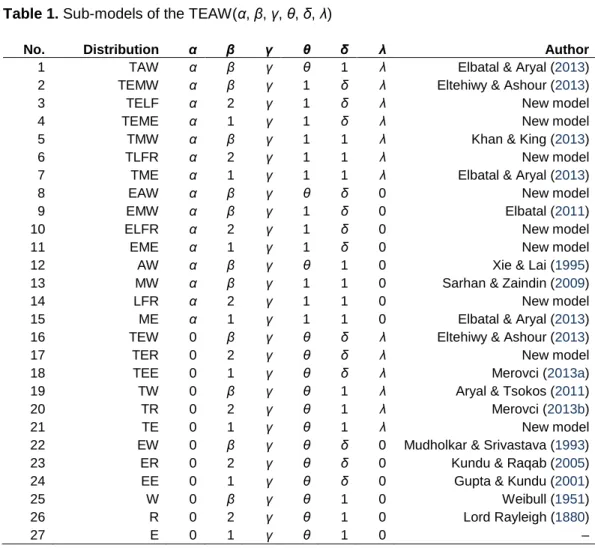
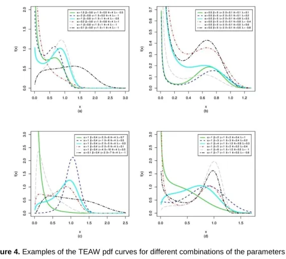
1 1 1 f ; e 1 e 1 2 1 e x x x x x x x x x − − − − − − − − − = + − + − − υ (10)The proposed TEAW model is a very flexible model that approaches to different distributions. It includes as special cases twenty-seven sub-models when its parameters vary. The flexibility of TEAW is explained in Table 1 and some examples of the pdf can be visualized in Figure 4 in Appendix A.
Table 1. Sub-models of the TEAW(α, β, γ, θ, δ, λ)
No. Distribution α β γ θ δ λ Author
1 TAW α β γ θ 1 λ Elbatal & Aryal (2013)
2 TEMW α β γ 1 δ λ Eltehiwy & Ashour (2013)
3 TELF α 2 γ 1 δ λ New model
4 TEME α 1 γ 1 δ λ New model
5 TMW α β γ 1 1 λ Khan & King (2013)
6 TLFR α 2 γ 1 1 λ New model
7 TME α 1 γ 1 1 λ Elbatal & Aryal (2013)
8 EAW α β γ θ δ 0 New model
9 EMW α β γ 1 δ 0 Elbatal (2011)
10 ELFR α 2 γ 1 δ 0 New model
11 EME α 1 γ 1 δ 0 New model
12 AW α β γ θ 1 0 Xie & Lai (1995)
13 MW α β γ 1 1 0 Sarhan & Zaindin (2009)
14 LFR α 2 γ 1 1 0 New model
15 ME α 1 γ 1 1 0 Elbatal & Aryal (2013)
16 TEW 0 β γ θ δ λ Eltehiwy & Ashour (2013)
17 TER 0 2 γ θ δ λ New model
18 TEE 0 1 γ θ δ λ Merovci (2013a)
19 TW 0 β γ θ 1 λ Aryal & Tsokos (2011)
20 TR 0 2 γ θ 1 λ Merovci (2013b)
21 TE 0 1 γ θ 1 λ New model
22 EW 0 β γ θ δ 0 Mudholkar & Srivastava (1993)
23 ER 0 2 γ θ δ 0 Kundu & Raqab (2005)
24 EE 0 1 γ θ δ 0 Gupta & Kundu (2001)
25 W 0 β γ θ 1 0 Weibull (1951)
26 R 0 2 γ θ 1 0 Lord Rayleigh (1880)
27 E 0 1 γ θ 1 0 –
Note the procedure of adding one or two shape parameters to a baseline distribution by using an adequate generator, in this particular case two extra shape parameters, will add more flexibility to the generated TEAW distribution since it can provide a large range for the skewness and great variability for the tail weights. The main motivation of the TEAW model is illustrated by considering a device made of δ parallel components for which the lifetime of each component is an AW random variable with cdf (1). The device fails if all δ components fail and, to improve the reliability of this device, we have to duplicate each component in parallel form, in which case the life of the device is governed by the cdf (9) at λ = -1. Furthermore, consider a system consisting of δ independent components that are connected in parallel with each component consisting of two units. If the two
units are connected in series, then the overall system will have the TEAW model with λ = 1, whereas if the two units are connected in parallel then λ = -1.
Another physical motivation for the TEAW model follows by taking two independent and identically distributed random variables, say Z1 and Z2, with cdf
G(x) = (1 – e-αxθ-γxβ)δ. Let Z1:2 = min(Z1, Z2) and Z2:2 = max(Z1, Z2). Next, consider
the random variable X defined by
1:2 2:2 1 with probability 2 1 with probabilit , y 2 , Z X Z + = −
Finally, the cdf of X is given by (9).
Mixture Representation for the TEAW pdf
Expansions for equation (10) can be derived using the series expansion
(
)
( ) (
(
)
)
0 1 1 1 , 1, 0 ! 1 j k j j k z z z k j k j = − + − = − +
(11)where Γ(∙) is the Gamma function. The pdf (10) can be rewritten as
( )
(
)
( )(
)
( )(
)
( )(
)
( ) 1 1 1 1 A B 1 1 f ; 1 e 1 e 2 1 e 1 e x x x x x x x x x x x x x − − + − − − + − − + − − − + = + + − − + + − υ (12)By expanding the quantities A and B in series expansion and, after some algebra, we have
( )
( ) (
(
) (
)
)
(
)
( )( )( )
( )
(
)
(
)
( )( ) 1 1 1 0 1 1 1 1 0 1 1 1 f ; e ! 1 2 2 e ! 2 j j x x j j j x x j x x x j j x x j j − + + − − = + − + + − − = − + + = + − − + + −
υ (13)Then the pdf of the TEAW in equation (10) can be expressed in the mixture form
( )
1( )
1( )
0 0 f ; j j j j j j x a g x b g x + + = = =
+
υ (14) where( ) (
) (
)
(
)
( )
(
( )
)
1 0 0 1 1 1 1 2 2 , ! ! 2 j j j j j j a b j j j j + = = − + + − = = − −
and(
)
(
1 1)
( )1( ) 1 1 e j x x j g j x x − − − − + + = + +is the pdf of the random variable Zj+1 ~ AW(α(j + 1), β, γ(j + 1), θ). Let pj = aj + bj.
Then the equation (14) can be expressed as
( )
1( )
0 f ; j j j x p g x + = =
υ (15)Equation (15) reveals that the TEAW density function can be expressed as a mixture of AW densities with different scale parameters. Thus, some of its mathematical properties can be obtained directly from the properties of the AW distribution.
Some Statistical Properties
Established algebraic expansions to determine some structural properties of the TEAW distribution can be more efficient than computing those directly by
numerical integration of its density function. The statistical properties of the TEAW distribution including quantile function (qf) and ordinary and incomplete moments are discussed in this section.
Quantile Function and Moments
The qf of X, where X ~ TEAW(α, β, γ, θ, δ, λ), is obtained by inverting (9) as
(
) (
)
2 1 1 4 ln 1 0 2 q q q x x + − + − + + − = (16)Since the above equation has no closed form solution in xq, we have to use numerical methods to obtain the quantiles.
Also, the rth moment of X, denoted by r0, is given by the following theorem:
Theorem 1. If X is a continuous random variable with TEAW(α, β, γ, θ, δ, λ), then the qth non-central moment of X is given by
( )
(
)
(
1, 1,)
0 E q 1 q j q j q j j X j p I I + − + − = = =
+ + (17)where I is determined by the following integral:
(
)
(
)
(
)
( 1)( ) , 0 ; 1 , , 1 , k n e j x x k j I I k j j x dx + − + + = + + =
(18)Proof. We can determine q from equation (17) by expanding
( 1 )
e−x j+ in power series; the above equation reduces to
( )
(
)
( ) ( )( )
(
)
1 , 0 0 1 0 1 1 e ! 1 1 1 1 ! n n j x k n k j n n n k n a j I x dx n a j k n n − + + = + = − + = − + + + =
(19)Consider the complex parameter Wright generalized hypergeometric function with p numerator and q denominator parameters defined by
(
)
(
)
(
)
(
)
(
)
(
)
1 1 1 0 1 1 1 , , , , , ; , ! , , , , p n p p j j j p q q n j j p p j A A A n z z B n n B B = = = =
Ψ (20)Then equation (19) can be expressed in a simple form, provided that β > 1, using the Wright generalized hypergeometric function. This yields
( )
(
)
, 1 1 0 1 , 1 1 ; k j k k a j I + + + = − − Ψ (21)Applying (21) to equation (17) gives (for q≥ 1)
(
)
(
1, 1,)
0 1 q j q j q j j j p I I + − + − = =
+ + (22)The moment generating function (mgf) of X, MX(t), is given by
( )
(
)
(
1, 1,)
, 0 M 1 ! q X j q j q j q j t t j p I I q + − + − = =
+ + (23)The nth central moment of X, n =E
(
X −1)
n (for n ≥ 1), is given by(
1)(
)
(
1, 1,)
, 0 1 ! q n n j q j q j q j n t j p I I k q + − + − = = − + +
(24)The variance, skewness, kurtosis, and higher-order cumulants of X can be determined from the central moments using well-known relationships.
Incomplete Moments
The main application of the first incomplete moment refers to the Bonferroni and Lorenz curves. These curves are very useful in economics, reliability, demography,
insurance, and medicine. Another application of the first incomplete moment is related to the mean residual life and the mean waiting time (also known as mean inactivity time) given by m1(t; υ) = (1 – φ1(t)) / (1 – F(t; υ)) – t and
M1(t; υ) = t – φ1(t) / F(t; υ), respectively.
The sth incomplete moment of X is
( )
( )
0 φ f t s s t =
x x dx Henceforth, let(
)
( )1 0 P ; , e t j x s t s j =
x − + dxWe obtain from equation (15)
( )
(
1 1)
( 1)( ) 0 φ e t j x x s s t x x x dx − − − + + =
+ (25) By expanding e (j 1)( x x ) − + + , we have( )
(
)
( )
(
)
(
)
, 0 1 φ P ; 1, 1 ! P ; 1, q j s q j q p a j t t s q j q t s q j = + = + + − − + + + −
(26) where(
)
1(
)
( )1 1 P ; ,t s j j 1 s γ s ,t + − + = + and( )
1 0 γ , e t y a t =
y− − dyis the lower incomplete gamma function.
The amount of scatter in a population is evidently measured to some extent by the totality of deviations from the mean and median. The mean deviations about the mean μ
(
δ( )
X =E(
X −10)
)
and the median M(
δM( )
X =E(
X−M)
)
ofX can be, used as measures of spread in a population, expressed by
( )
0( )
0( )
0( )
0 1 1 1 1 1 0 δ X X f x dx 2 F 2φ =
− = − (27) and( )
( )
0( )
1 1 0 δM X X M f x dx 2 2φ M =
− = − (28)respectively, where 10=E
( )
X comes from equation (17), F( )
10 is simply calculated from equation (9), and φ1( )
10 is the first incomplete moment.The application of mean deviations refers to the Lorenz and Bonferroni curves defined by L
( )
p =φ1( )
q 10 and B( )
p =φ1( )
q p10 , respectively, where q = F-1(p) can be computed for a given probability p by inverting equation (9) numerically (Pescim, Cordeiro, Nararajah, Demetrio, & Ortega, 2014).Reliability Analysis
The characteristics in reliability analysis which are the reliability function (rf), hazard rate function (hrf), cumulative hazard rate function (chrf), moments of the residual life, and moments of the reversed residual life for the TEAW distribution are introduced in this section.
Reliability, Hazard Rate, and Cumulative Hazard Rate Functions
The rf is the probability of an item not failing prior to some time t. The rf of X is given by
( )
(
)
(
)
R x; 1 1 e x x 1 1 e x x − − − − = − − + − − υ (29)The hrf is important in a number of applications and is known by a variety of names. It is used by actuaries under the name force of mortality to compute mortality tables. In statistics, its reciprocal for the normal distribution is known as Mills’ ratio. It plays an important role in determining the form of extreme value distributions, and in extreme value theory is called the intensity function. The hrf of X is an important quantity characterizing life phenomenon and it is defined by
( )
(
)
(
)
(
)
(
)
(
)
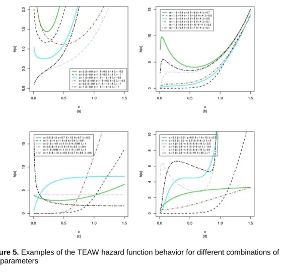
1 1 1 h ; e 1 e 1 2 1 e 1 1 e 1 1 e x x x x x x x x x x x x x − − − − − − − − − − − − − = + − + − − − − + − − υ (30)Some examples of the hazard curves can be found in Appendix A, Figure 5. It is important to note that the units for h(x; υ) are the probability of failure per unit of time, distance, or cycles. These failure rates are defined with different choices of parameters. The chrf of X is defined by
( )
(
)
(
)
H x; ln 1 1 e x x 1 1 e x x − − − − = − − − + − − υ (31)It is important to note that the units for H(x; υ) are the cumulative probability of failure or death per unit of time, distance, or cycles.
Moments of the Residual Life
Several functions are defined related to the residual life: the failure rate function, mean residual life function, and the left-censored mean function, also called vitality function. These three functions uniquely determine F(x) (see, e.g., Gupta, 1975;
Definition 3. Let X be a random variable, usually representing the life length for a certain unit at age t (where this unit can have multiple interpretations); then the random variable Xt = X – t∣ X > t represents the remaining lifetime beyond that age.
Moreover, the nth moments of residual life, denoted by
mn(t) = E((X – t)n∣ X > t), n = 1, 2, 3,…, uniquely determine F(x) (see Navarro, Franco, & Ruiz, 1998). The nth moments of the residual life of a random variable are given by
( )
1( ) (
)
( )
m F 1 F n n t t x t d x t = − −
(32)Therefore, the nth moments of the residual life of X are given by
( )
( )
( )
(
)
(
)
(
)
(
)
0 0 1 ! 1 m 1 R ! ! ! P ; 1, P ; 1, n q r n r n q j n r q n t t p a j t r q n r t n q j t n q j + − − = = − = + − + + − + + + −
(33)Another interesting function is the mean residual life function (MRL), or the life expectancy at age x, defined by m1(t) = E((X – t) ∣ X > t), which represents the
expected additional life length for a unit which is alive at age x. The MRL of the distribution can be obtained by setting n = 1 in (33).
Guess and Proschan (1988) provided an extensive coverage of possible applications of the mean residual life. The MRL has many applications in survival analysis in biomedical sciences, life insurance, maintenance and product quality control, economics and social studies, demography, and product technology (see, e.g., Lai & Xie, 2006).
Moments of the Reversed Residual Life
The nth moments of the reversed residual life, denoted by Mn(t) = E((t – X)n∣ X ≤ t), t > 0, n = 1, 2, 3,…, uniquely determine F(x). The nth moments of the reversed residual life random variable are given by
( )
( ) (
)
( )
0 1 M F F t n n t t x d x t =
− (34)Therefore, the nth moments of the reversed residual life of X can be expressed, in a similar manner, as
( )
( )
( )
(
)
(
)
(
)
(
)
0 0 1 ! 1 M 1 F ! ! ! P ; 1, P ; 1, r q n r n q j n t q n t t p a j t r q n r t n q j t n q j + − = = − = + − + + − + + + −
(35)The mean inactivity time (MIT), also called mean reversed residual life function, defined by M1(t) = E((t – X) ∣ X ≤ t), represents the waiting time elapsed since the
failure of an item on condition that this failure had occurred in (0, t). The MIT of the TEAW distribution can be obtained by setting n = 1 in equation (35). The properties of the mean inactivity time have been considered by many authors (see, e.g., Kayid & Ahmad, 2004; Ahmad, Kayid, & Pellerey, 2005).
Order Statistics
The order statistics and their moments have great importance in many statistical problems and have many applications in reliability analysis and life testing. The order statistics arise in the study of reliability of a system. The order statistics can represent the lifetimes of units or components of a reliability system. Let X1, X2,…,
Xn be a random sample of size n from the TEAW distribution with cdf and pdf as in (9) and (10), respectively. Let X(1), X(2),…, X(n) be the corresponding order
statistics. Then the pdf of ith order statistic, say Xi:n, 1 ≤ i ≤ n, denoted by fi:n(x), is
given by
( )
(
)
(
)
(
)
(
)
(
)
(
)
1 1 1 : 1 f e 1 e 1 1 e 1 2 1 e 1 1 e 1 1 e x x x x i n i x x x x n i x x x x n x x x i − − − − − − − − − − − − − − − − − = + − + − − + − − − − + − − (36)( )
(
( )
) ( )
( )
1 : 0 f f 1 F B , 1 j j i i n q n i x x x j i n i + − = − = − − +
(37)where B(∙) is the Beta function. After some simplification, we can write
( ) ( )
1( )
( )
1 1 0 0 f F j i mgm mgm m m x x d x s x + − + + = = =
+
(38) where( )
(
)
(
)
(
)
(
) (
)
(
)
( )
(
)
(
)
(
)
(
) (
)
(
)
0 1 1 1 0 1 1 ! 1 ! 1 1 1 ! 1 ! 1 m j i m j i m j i j i d m j i j i m j i j i s m j i j i m + + − = + + + − − = − + + + + = + + − + + − − + + + + + = + + − + + + −
Equation (38) can be expressed as
( ) ( )
1( )
1 0 f F j i mgm m x x t x + − + = =
(39) where tm = dm + sm.By inserting (39) in equation (37), we obtain
( )
( )
(
)
( )
: 1 0 1 f g B , 1 j i n m m m n i j x t x i n i + = − − = − +
(40)where gm+1(x) is the AW density function with parameters α(m + 1), β, γ(m + 1),
and θ.
Equation (40) reveals that the pdf of the TEAW order statistics is a mixture of AW densities. Some of their mathematical properties can also be obtained from those of the AW distribution. For example, the qth moment of Xi:n can be expressed
( )
:( )
(
) (
)
(
1, 1,)
0 0 1 E 1 B , 1 j n i q i n m q m q m j m n i j X m t I I i n i − + − + − = = − − = + + − +
(41)Based upon the moments (41), derive explicit expressions for the L-moments of X as infinite weighted linear combinations of the means of suitable AW distributions. They are linear functions of expected order statistics defined by
( )
(
)
1 : 0 1 1 1 E , 1 r d r r d d d r X r d r − − = − = −
(42)The first four L-moments are given by
( )
(
)
(
)
(
)
1 1:1 2 2:2 1:2 3 3:3 2:3 1:3 4 4:4 3:4 2:4 1:4 1 E E 2 1 1 E 2 E 3 3 3 4 X X X X X X X X X X = = − = − + = − + −One simply can obtain the λs for X from equation (39) with q = 1.
Maximum Likelihood Estimation
The maximum likelihood estimators (MLEs) for the parameters of the TEAW distribution are discussed in this section. Let X = (X1, X2,…, Xn) be a random
sample of this distribution with unknown parameter vector υ = (α, β, γ, θ, δ, λ)T. The likelihood function for υ is
( )
(
)
1 L n e si 1 e si n n n n i q i q i i q i q i z k = = − − − = = =
−
υ (43) where zi = αθxθ-1 + γβxβ-1, si = αxθ + γxβ, and 1 2(
1 e si)
i k = + − − − . Then the log-likelihood function ℓ = ln L(υ) is given by( )
( ) (
)
(
)
( )
1 1 1 1 ln ln 1 ln 1 e i ln n n n n s i i i i i i i n s z − k = = = = = −
+ + −
− +
(44)The components of the score vector
( )
T U , , , , , = = υ υ are given by(
)
(
)
1 1 1 1 1 1 e 1 e e 1 2 1 e i i i i s s s n n n n i i i i s i i i i i i x x x x z k − − − − − − = = = = − = − + − −
−
(45)(
)
(
( )
)
( )
(
)
( )
1 1 1 1 1 1 ln 1 ln 1 ln 1 e 1 e e ln 2 i i i n n n i i i i i i s i i i i s s n i i i i i x x x s x x z s x x k − − = = = − − − = + = − + + − − −
(46)(
)
(
)
1 1 1 1 1 1 e 1 e e 1 2 1 e i i i i s s s n n n n i i i i s i i i i i i x x x x z k − − − − − − = = = = − = − + − −
−
(47)(
)
( )
(
( )
)
( )
(
)
( )
1 1 1 1 1 1 ln 1 e ln 1 ln 1 e 1 e ln 2 i i i i s n n n i i i i i i s i i i i s s n i i i i x x x x x x z x e x k − − − = = = − − − = + = − + − − − −
(48)(
)
(
) (
)
1 1 1 e ln 1 e ln 1 e 2 i i i s s n n s i i i n k − − − = = − − = + − −
(49) and(
)
1 1 2 1 e si n i ki − = − − =
(50)Find the estimates of the unknown parameters by setting the score to zero, i.e., by solving the nonlinear system of equations: U
( )
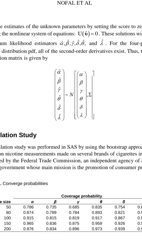
υˆ =0. These solutions will yield the maximum likelihood estimators ˆ, , , , ,ˆ ˆ ˆ ˆ and ˆ . For the four-parameters TEAW distribution pdf, all of the second-order derivatives exist. Thus, the inverse dispersion matrix is given by~ , ˆ ˆ ˆ ˆ ˆ ˆ N
Simulation Study
A simulation study was performed in SAS by using the bootstrap approach. It was based on nicotine measurements made on several brands of cigarettes in 1998 and collected by the Federal Trade Commission, an independent agency of the United States government whose main mission is the promotion of consumer protection.
Table 2. Converge probabilities
Coverage probability Sample size α β γ θ δ λ 50 0.786 0.735 0.685 0.835 0.754 0.857 80 0.874 0.789 0.784 0.893 0.821 0.935 100 0.915 0.815 0.819 0.917 0.867 0.952 150 0.965 0.836 0.875 0.959 0.926 0.976 200 0.976 0.834 0.896 0.973 0.939 0.984
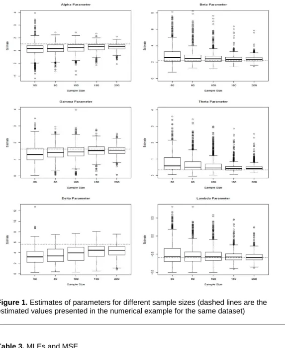
Figure 1. Estimates of parameters for different sample sizes (dashed lines are the estimated values presented in the numerical example for the same dataset)
Table 3. MLEs and MSE
Sample size Estimate MSE α β γ θ δ λ α β γ θ δ λ 50 1.107 3.040 1.292 0.798 3.256 -0.486 2.672 5.451 1.577 1.892 15.362 0.978 80 1.143 2.635 1.393 0.683 3.536 -0.531 2.397 2.091 1.366 1.514 13.781 0.753 100 1.199 2.541 1.442 0.607 3.864 -0.536 2.050 1.622 1.068 1.153 12.540 0.696 150 1.266 2.390 1.515 0.498 4.246 -0.559 1.702 0.833 0.780 0.768 10.528 0.572 200 1.285 2.349 1.532 0.470 4.318 -0.575 1.491 0.630 0.651 0.620 9.504 0.486
Presented in Table 3 are the mean of the MLEs and the mean square error (MSE). When the sample size increases, the MSE becomes smaller and the mean of the MLEs are close to the observed value in the second example. The example was performed by using the same dataset (nicotine data, Table 6, and the dashed lines presented in Figure 1). Shown in Table 2 are the coverage probabilities of the 95% two-sided confidence intervals for the model TEAW parameters. Although the convergence to the nominal value for the parameters β and γ is slow (there is a tendency for the nominal value as the sample size increases), for the parameters α, θ, δ, and λ, by considering sample size 200, the observed values are close to the nominal one, 95%.
Numerical Experiments
Two applications to real data to show the importance and usefulness of the TEAW model.
Application to Carbon Fibers Data
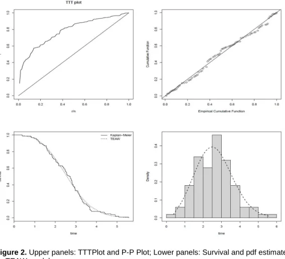
The data set that corresponds to an uncensored study on the breaking stress of carbon fibres (in Gba), from Nichols and Padgett (2006), was used. This data set was also used by Afify, Yousof, Cordeiro, Ortega, and Nofal (2016) to fit the Weibull Fréchet distribution. TTT Plot of times can be seen in Figure 2, upper left panel, which indicates a possible increase hazard.
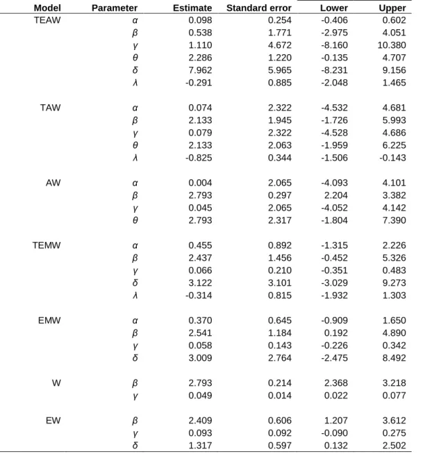
Shown in Table 4 are the MLEs to seven nested distributions: TEAW (transmuted exponential additive Weibull), TAW (transmuted additive Weibull), AW (additive Weibull), TEMW (transmuted exponential modified Weibull), EMW (exponential modified Weibull), W (Weibull), and EW (exponential Weibull). Also presented for all models, in Table 5, are two different statistics of fit that were used as selection criteria: -2 × log-likelihood (-2log) and the likelihood ratio (LR) test.
The calculated values of these statistics (the smaller the better) show us that the adjustments of all models are close. Also, the p-values are presented for the likelihood ratio test comparing the sub-models to the TEAW model. Figure 2 shows the P-P Plot which indicates a good adjustment to the TEAW model. This quality of fit can be analyzed by the survival and density curves showed in the lower panels of Figure 2.
Table 4. MLEs of the parameters of some TEAWs nested models
CI (95%) Model Parameter Estimate Standard error Lower Upper
TEAW α 0.098 0.254 -0.406 0.602 β 0.538 1.771 -2.975 4.051 γ 1.110 4.672 -8.160 10.380 θ 2.286 1.220 -0.135 4.707 δ 7.962 5.965 -8.231 9.156 λ -0.291 0.885 -2.048 1.465 TAW α 0.074 2.322 -4.532 4.681 β 2.133 1.945 -1.726 5.993 γ 0.079 2.322 -4.528 4.686 θ 2.133 2.063 -1.959 6.225 λ -0.825 0.344 -1.506 -0.143 AW α 0.004 2.065 -4.093 4.101 β 2.793 0.297 2.204 3.382 γ 0.045 2.065 -4.052 4.142 θ 2.793 2.317 -1.804 7.390 TEMW α 0.455 0.892 -1.315 2.226 β 2.437 1.456 -0.452 5.326 γ 0.066 0.210 -0.351 0.483 δ 3.122 3.101 -3.029 9.273 λ -0.314 0.815 -1.932 1.303 EMW α 0.370 0.645 -0.909 1.650 β 2.541 1.184 0.192 4.890 γ 0.058 0.143 -0.226 0.342 δ 3.009 2.764 -2.475 8.492 W β 2.793 0.214 2.368 3.218 γ 0.049 0.014 0.022 0.077 EW β 2.409 0.606 1.207 3.612 γ 0.093 0.092 -0.090 0.275 δ 1.317 0.597 0.132 2.502
Figure 2. Upper panels: TTTPlot and P-P Plot; Lower panels: Survival and pdf estimated by TEAW model
Table 5. Measure of selection criteria
Criterias Model -2log LR p-value
TEAW 282.4 − TAW 282.7 0.4161 AW 283.1 0.2953 TEMW 282.5 0.2482 EMW 282.6 0.0952 W 283.1 0.0487 EW 282.7 0.0400
Table 6. MLEs of the parameters of some nested models and selection criteria
Selection Criteria
Model Parameter Estimate Standard error -2log AIC AICC BIC
TEAW α 1.528 1.048 214.7 226.7 227.0 249.8 β 2.229 0.292 -- -- -- -- γ 1.613 0.349 -- -- -- -- θ 0.345 0.244 -- -- -- -- δ 5.663 6.551 -- -- -- -- λ -0.592 0.336 -- -- -- -- TAW α 0.388 0.354 218.1 228.1 228.3 247.4 β 2.664 0.314 -- -- -- -- γ 1.172 0.347 -- -- -- -- θ 1.216 0.517 -- -- -- -- λ -0.708 0.213 -- -- -- -- AW α 0.426 0.167 217.6 225.6 225.8 241.0 β 2.652 0.235 -- -- -- -- γ 1.245 0.187 -- -- -- -- θ 0.700 0.221 -- -- -- -- TEMW α 0.722 0.501 217.1 227.1 227.2 246.3 β 2.599 0.272 -- -- -- -- γ 1.177 0.265 -- -- -- -- δ -0.629 0.230 -- -- -- -- λ 1.525 0.494 -- -- -- -- EMW α 0.453 0.305 218.9 226.9 227.0 242.3 β 2.841 0.216 -- -- -- -- γ 1.068 0.133 -- -- -- -- δ 1.626 0.424 -- -- -- -- W β 2.719 0.114 227.6 231.6 231.6 239.2 γ 1.047 0.022 -- -- -- -- EW β 3.063 0.354 226.3 232.3 232.4 243.9 γ 0.947 0.173 -- -- -- -- δ 0.812 0.152 -- -- -- --
Application to Nicotine Data
The second data set pertains to nicotine measurements made on several brands of cigarettes, collected by the Federal Trade Commission. Tar, nicotine, and carbon monoxide of the smoke of 1206 varieties of domestic cigarettes for the year of 1998 are recorded, along with some information about the source of the data; smokers’
behavior; and smokers’ beliefs about nicotine, tar, and carbon monoxide contents
in cigarettes. The free form data set can be found at
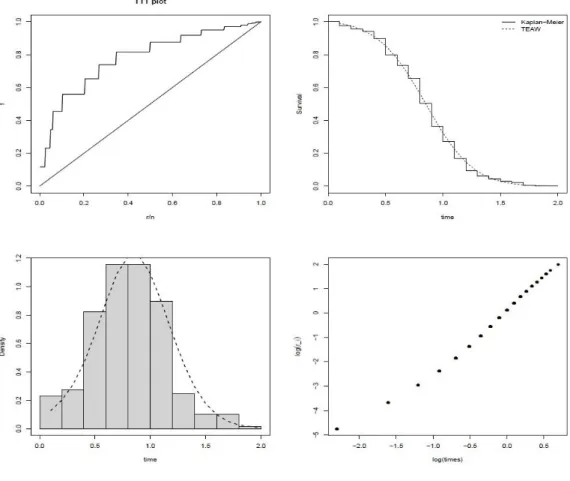
http://www.econdataus.com/smoke.html. The TTT Plot of the times can be seen in
Figure 2, upper left panel.
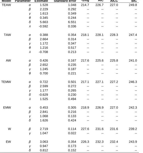
Compiled in Table 6 are the MLEs of seven nested distributions: TEAW (transmuted exponential additive Weibull), TAW (transmuted additive Weibull), AW(additive Weibull), TEMW (transmuted exponential modified Weibull), EMW (exponential modified Weibull), W (Weibull), and EW (exponential Weibull); four different statistics of fit were used as selection criteria: -2log, Akaike’s information criterion (AIC), corrected Akaike’s information criterion (AICC), and Schwarz Bayesian information criterion (BIC), that are given by:
(
)
( )
AIC 2 log 2 2 1 AICC 2 log 2 1 BIC 2 log f n logp p p p n p x p n = − + + = − + + − − = − +
where n is the sample size and p is the number of parameters.
The calculated values of these statistics (the smaller the better) show us that the TEAW model is better fitted than the others. Also, the quality of fit can be analyzed by the survival and density curves showed in Figure 3.
By considering four different criteria of selection, the TEAW model is the most appropriate to fit the data, which can be checked in Figure 2. In order to examine the global adjust of the model, a residual analysis was conducted, as in the examples by McCullagh and Nelder (1989), Barlow and Prentice (1988), and Therneau, Grambsch, and Fleming (1990). The first, the error used in Martingale-type residual, was introduced Therneau et al. and was used in a counting process. They are skewed and have a maximum value at +1 and a minimum value at -∞. The error of TEAW can be written as
( )
( )
log 1 ζ 1 ζ i i i r = − − t + − t (51) where ζ( )
ti 1 e ( x x ) − + = − , i = 1,…, nFigure 3, lower right panel, shows the plot of log ri versus where the global adjustment of the model is seen to be appropriate.
Figure 3. Upper panels: TTTPlot and Survival curves; Lower panels: pdf estimated by TEAW model and residual analysis
Conclusion
A new model, called the transmuted exponentiated additive Weibull (TEAW) distribution, was proposed which extends the TAW distribution introduced by Elbatal and Aryal (2013). An obvious reason for generalizing a standard distribution is that it provides more flexibility to analyze real-life data. The TEAW distribution is motivated by the wide use of the Weibull distribution in practice, and also for the fact that the generalization provides more flexibility to analyze real data. The TEAW density function can be expressed as a mixture of AW densities. Explicit expressions were derived for the ordinary and incomplete moments and generating function, moments of residual, and reversed residual life. The density function of the order statistics and their moments were obtained, and the inference
section presents the maximum likelihood estimation procedure. Two applications illustrate that the new model provides consistently good fit. The TEAW model has several sub-models, and works as a comprehensive model which is a unique algorithm to fit a large number of models. It is shown, from the plots of the pdf and hazard function of the TEAW model, this distribution is very flexible, accommodating a large number of shapes for the hazard function.
References
Afify, A. Z., Cordeiro, G. M., Yousof, H. M., Saboor, A., & Ortega, E. M. M. (in press). The Marshall-Olkin additive Weibull distribution with variable shapes for the hazard rate. Hacettepe Journal of Mathematics and Statistics. doi:
10.15672/hjms.201612618532
Afify, A. Z., Hamedani, G. G., Ghosh, I., & Mead, M. E. (2015). The transmuted Marshall-Olkin Fréchet distribution: Properties and applications. International Journal of Statistics and Probability, 4(4), 132-148. doi:
10.5539/ijsp.v4n4p132
Afify, A. Z., Nofal, Z. M., & Butt, N. S. (2014). Transmuted complementary Weibull geometric distribution. Pakistan Journal of Statistics and Operations Research, 10(4), 435-454. doi: 10.18187/pjsor.v10i4.836
Afify, A. Z., Yousof, H. M., Cordeiro, G. M., Ortega, E. M., & Nofal, Z. M. (2016). The Weibull Fréchet distribution and its applications. Journal of Applied Statistics, 43(14), 2608-2626. doi: 10.1080/02664763.2016.1142945
Ahmad, I., Kayid, M., & Pellerey, F. (2005). Further results involving the MIT order and the IMITclass. Probability in the Engineering and Informational Science, 19(3), 377-395. doi: 10.1017/s0269964805050229
Aryal, G. R., & Tsokos, C. P. (2009). On the transmuted extreme value distribution with application. Nonlinear Analysis: Theory, Methods &
Applications, 71(12), 1401-1407. doi: 10.1016/j.na.2009.01.168
Aryal, G. R., & Tsokos, C. P. (2011). Transmuted Weibull distribution: a generalization of the Weibull probability distribution. European Journal of Pure and Applied Mathematics, 4(2), 89-102. Retrieved from
https://www.ejpam.com/index.php/ejpam/article/view/1170
Barlow, W. E., & Prentice, R. L. (1988). Residuals for relative risk regression. Biometrika, 75(1), 65-74. doi: 10.1093/biomet/75.1.65
Elbatal, I. (2011). Exponentiated modified Weibull distribution. Economic Quality Control, 26(2), 189-200. doi: 10.1515/eqc.2011.018
Elbatal, I., & Aryal, G. (2013). On the transmuted additive Weibull distribution. Austrian Journal of Statistics, 42(2), 117-132. doi:
10.17713/ajs.v42i2.160
Eltehiwy, M., & Ashour, S. (2013). Transmuted exponentiated modified Weibull distribution. International Journal of Basic and Applied Sciences, 2(3), 258-269. doi: 10.14419/ijbas.v2i3.1074
Granzotto, D. C. T., & Louzada, F. (2015). The transmuted log-logistic distribution: Modeling, inference and an application to a polled Tabapua race time up to first calving. Communications in Statistics – Theory and Methods, 44(16), 3387-3402. doi: 10.1080/03610926.2013.775307
Guess, F., & Proschan, F. (1988). Mean residual life: Theory and
applications. In P. R. Krishnaiah & C. R. Rao (Eds.), Handbook of statistics (Vol. 7) (pp. 215-224). New York, NY: North-Holland. doi:
10.1016/s0169-7161(88)07014-2
Gupta, R. (1975). On characterization of distribution by conditional expectation. Communications in Statistics, 4(1), 99-103. doi:
10.1080/03610927508827230
Gupta, R. D., & Kundu, D. (2001). Exponentiated exponential family: An alternative to gamma and Weibull distributions. Biometrical Journal, 43(1), 117-130. doi: 10.1002/1521-4036(200102)43:1<117::aid-bimj117>3.0.co;2-r
Kayid, M., & Ahmad, I. (2004). On the mean inactivity time ordering with reliability applications. Probability in the Engineering and Informational
Sciences, 18(3), 395-409. doi: 10.1017/s0269964804183071
Khan, M. S., & King, R. (2013). Transmuted modified Weibull distribution: A generalization of the modified Weibull probability distribution. European Journal of Pure and Applied Mathematics, 6(1), 66-86. Retrieved from
https://www.ejpam.com/index.php/ejpam/article/view/1606
Kotz, S., & Shanbhag, D. N. (1980). Some new approaches to probability distributions. Advances in Applied Probability, 12(4), 903-921. doi:
10.1017/s0001867800020164
Kundu, D., & Raqab, M. Z. (2005). Generalized Rayleigh distribution: Different methods of estimations. Computational Statistics & Data Analysis, 49(1), 187-200. doi: 10.1016/j.csda.2004.05.008
Lai, C. D. & Xie, M. (2006). Stochastic ageing and dependence for reliability. New York, NY: Springer. doi: 10.1007/0-387-34232-x
Lai, C. D., Xie, M., & Murthy, D. N. P. (2001). Bathtub-shaped failure rate life distributions. In N. Balakrishnan & C. R. Rao (Eds.), Handbook of statistics (Vol. 20) (pp. 69-104). New York, NY: Elsevier North Holland. doi:
10.1016/s0169-7161(01)20005-4
Lai, C. D., Xie, M., & Murthy, D. N. P. (2003). A modified Weibull distribution. IEEE Transactions on Reliability, 52(1), 33-37. doi:
10.1109/tr.2002.805788
Lord Rayleigh. (1880). XII. On the resultant of a large number of vibrations of the same pitch and of arbitrary phase. The London, Edinburgh, and Dublin Philosophical Magazine and Journal of Science. Fifth Series, 10(60), 73-78. doi:
10.1080/14786448008626893
Louzada, F., & Granzotto, D. C. T. (2016). The transmuted log-logistic regression model: A new model for time up to first calving of cows. Statistical Papers, 57(3), 623-640. doi: 10.1007/s00362-015-0671-5
McCullagh, P., & Nelder, J. A. (1989). Generalized linear models (2nd ed.). London, UK: Chapman & Hall.
Merovci, F. (2013a). Transmuted exponentiated exponential distribution. Mathematical Sciences and Applications E-Notes, 1(2), 112-122. Retrieved from
http://www.mathenot.com/matder/dosyalar/makale-116/14merovci.pdf
Merovci, F. (2013b). Transmuted Rayleigh distribution. Austrian Journal of Statistics, 42(1), 21-31. doi: 10.17713/ajs.v42i1.163
Mudholkar, G. S., & Srivastava, D. K. (1993). Exponentiated Weibull family for analyzing bathtub failure rate data. IEEE Transactions on Reliability, 42(2), 299-302. doi: 10.1109/24.229504
Nadarajah, S. (2009). Bathtub-shaped failure rate functions. Quality & Quantity, 43(5), 855-863. doi: 10.1007/s11135-007-9152-9
Navarro, J., Franco, M., & Ruiz, J. (1998). Characterization through moments of the residual life and conditional spacing. Sankhyā: The Indian Journal of Statistics, Series A, 60(1), 36-48. Available from
http://www.jstor.org/stable/25051181
Nichols, M. D., & Padgett, W. J. (2006). A bootstrap control chart for Weibull percentiles. Quality and Reliability Engineering International, 22(2), 141-151. doi: 10.1002/qre.691
Pescim, R. R., Cordeiro, G. M., Nararajah, S., Demetrio, C. G. B., & Ortega, E. M. M. (2014).The Kummer beta Birnbaum-Saunders: An alternative fatigue life distribution. Hacettepe Journal of Mathematics and Statistics, 43(3), 473-510. Retrieved from http://www.hjms.hacettepe.edu.tr/uploads/1b448a5b-4698-4b06-bd14-4196db0e13e8.pdf
Sarhan, A. M., & Zaindin, M. (2009). Modified Weibull distribution. Applied Sciences, 11(1), 123-136.
Shaw, W. T., & Buckley, I. R. C. (2007, March 23). The alchemy of probability distributions: Beyond Gram-Charlier expansions, and a skew-kurtotic-normal distribution from a rank transmutation map. Presented at the IMA Conference on Computational Finance, London, UK.
Therneau, T. M., Grambsch, P. M., & Fleming, T. R. (1990). Martingale-based residuals for survival models. Biometrika, 77(1), 147-160. doi:
10.1093/biomet/77.1.147
Weibull, W. (1951). A statistical distribution function of wide applicability. Journal of Applied Mechanics, 18(3), 293-297.
Xie, M. & Lai, C. D. (1995). Reliability analysis using an additive Weibull model with bathtub-shaped failure rate function. Reliability Engineering & System Safety, 52(1), 87-93. doi: 10.1016/0951-8320(95)00149-2
Zoroa, P., Ruiz, J., & Marin, J. (1990). A characterization based on conditional expectations. Communications in Statistics – Theory and Methods, 19(6), 3127-3135. doi: 10.1080/03610929008830368
Appendix A – Complementary Figures
Some plots of the TEAW pdf and hrf are provided that show the flexibility of the TEAW model. Moreover, the TEAW model due to its flexibility in accommodating all forms of the hazard rate as follows.
Figure 5. Examples of the TEAW hazard function behavior for different combinations of the parameters