R. Smit, P. Kingston, D.H. Wainwright, R. Tooker PII: S1352-2310(16)30973-6
DOI: 10.1016/j.atmosenv.2016.12.014 Reference: AEA 15076
To appear in: Atmospheric Environment
Received Date: 22 September 2016 Revised Date: 27 October 2016 Accepted Date: 5 December 2016
Please cite this article as: Smit, R., Kingston, P., Wainwright, D.H., Tooker, R., A tunnel study to validate motor vehicle emission prediction software in Australia, Atmospheric Environment (2017), doi: 10.1016/ j.atmosenv.2016.12.014.
This is a PDF file of an unedited manuscript that has been accepted for publication. As a service to our customers we are providing this early version of the manuscript. The manuscript will undergo copyediting, typesetting, and review of the resulting proof before it is published in its final form. Please note that during the production process errors may be discovered which could affect the content, and all legal disclaimers that apply to the journal pertain.
M
AN
US
CR
IP
T
AC
CE
PT
ED
A tunnel study to validate motor vehicle emission prediction software in Australia
1
R. Smit a,b*, P. Kingston a, D.H. Wainwright a, R. Tooker a 2
a
Department of Science, Information Technology and Innovation (DSITI), GPO Box 5078, Brisbane, Q4001, 3
Australia 4
b
University of Queensland, Centre for Transport Strategy, Brisbane, Australia 5
* Corresponding author, phone +61 7 3170 5473, fax +61 7 3170 5797, e-mail [email protected] 6
Abstract
7
A tunnel emissions study was conducted to (partially) validate the Australian vehicle emissions software 8
COPERT Australia and PIARC emission factors. The in-tunnel fleet mix differs substantially from the average 9
on-road fleet, leading to lower emissions by factor of about 2. Simulation with the P∆P software found that in-10
tunnel air-flow roughly compensates for road gradient impacts on NOx emissions. PIARC emission factors are
11
conservative and exhibit the largest prediction errors, except for one very good agreement for LDV NOx.
12
COPERT Australia is generally accurate at fleet level for CO, NOx, PM2.5 and PM10, when compared with other
13
international studies, and consistently underestimates emissions by 7% to 37%, depending on the pollutant. 14
Possible contributing factors are under-representation of high/excessive emitting vehicles, inaccurate mileage 15
correction factors, and lack of empirical emissions data for Australian diesel cars. The study results demonstrate 16
a large uncertainty in speciated VOC and PAH emission factors. 17
Graphical abstract
18
19 20
M
AN
US
CR
IP
T
AC
CE
PT
ED
Highlights 21• Tunnel studies are useful to partially validate vehicle emissions software 22
• Air flow in tunnels can compensate the impacts of road gradients on vehicle emissions 23
• Local fleet mix is an essential factor in validation studies 24
Keywords
25
Motor vehicle; emissions; tunnel; validation; road traffic 26
1. Introduction
27
Motor vehicles are a major source of air pollution and greenhouse gas (GHG) emissions in urban areas around 28
the world. The close proximity of motor vehicles to the general population makes this a particularly relevant 29
source from an exposure and health perspective. This is illustrated by Caiazzo et al. (2013) who estimated that 30
total combustion emissions (particulates, ozone) in the U.S. account for about 210,000 premature deaths per 31
year, with motor vehicles being the largest contributor, contributing to around 58,000 premature deaths per year, 32
despite the fact that road transport only contributes about 7% to total PM2.5 emissions.
33
Comprehensive measurement of vehicle emissions in urban networks is cost prohibitive due to the large number 34
of vehicles that operate on roads with different emission profiles, large spatial and temporal variability in vehicle 35
activity and many real-world factors that influence emission levels (Smit et al., 2008). The environmental 36
impacts of road traffic are therefore commonly evaluated at different scales using transport and emission models 37
and, in the case of air pollution, dispersion and exposure models. Models are also required to make projections 38
into the future. 39
Vehicle-emission prediction software is well-established in Europe and the US. However, these models have 40
been found to not adequately represent Australian conditions in terms of fleet mix, vehicle technology, fuel 41
quality and climate. Large errors of up to a factor of 20 have been reported when overseas models were directly 42
applied to Australian conditions without calibration (Smit and McBroom, 2009). Therefore, two software 43
packages have been developed specifically for Australian conditions, using comprehensive empirical data from 44
major Australian laboratory emission testing programs. COPERT Australia has been developed to estimate 45
M
AN
US
CR
IP
T
AC
CE
PT
ED
motor vehicle emissions at a regional and national level, while a power-based model (P∆P) was developed for 46
local assessments, as will be discussed in section 2.2. 47
As models are simplifications of reality, their limitations and accuracy should be clearly established. This paper 48
presents results of a tunnel emissions study that was conducted in Brisbane, Australia. 49
2. Method
50
2.1 Tunnel studies 51
There are several methods used to (partially) validate vehicle emission models, such as on-board emission 52
measurements (PEMS), remote sensing, near-road air quality measurements and tunnel studies (Smit et al., 53
2010). Like all validation methods, tunnel studies have specific strengths and weaknesses. A strength is that 54
emissions are derived from a large sample of the on-road fleet under relatively controlled conditions, thereby 55
adequately capturing inter-vehicle variability in emissions. The spatial resolution aligns better with distance-56
based emission factors (g/km) commonly used in vehicle emission models, as compared with localised 57
validation methods such as remote sensing and near-road air quality measurements. 58
However, there are also some challenges with tunnel studies. They represent only a limited range of operating 59
conditions (typically ‘smooth’, uncongested, high-speed driving). As a consequence, validation results cannot be 60
directly translated, for example, to commonly occurring urban driving conditions at lower speeds. Tunnels may 61
also have significant uphill and downhill gradients, and in-tunnel air-flows affecting emissions. Furthermore, 62
assumptions relating to the unknown proportion of vehicles in cold-start mode and actual vehicle loads are 63
required to make a comparison with model predictions. Nevertheless, tunnel studies provide a useful approach to 64
(partially) validate vehicle emission models for specific traffic situations. 65
Tunnel studies have been extensively used around the world to compare model predictions with observed values 66
(e.g. De Fré et al., 1994; Hausberger et al., 2003; Geller et al., 2005). In these studies, emission factors, 67
expressed as grams of pollutant per vehicle kilometre (g/veh.km, subsequently denoted as g/km), are determined 68
using the differences between the concentration levels at the tunnel entrance and exit, combined with tunnel 69
features (e.g. road length), traffic flow and traffic conditions, as well as either measured tunnel air-flow or a 70
dilution factor based on a tracer gas (e.g. SF6). Regression analysis is often used to develop mean emission
71
factors (g/km) by time of day for basic vehicle classes (e.g. light-duty vehicle, LDV and heavy-duty vehicle, 72
HDV). License plate information is typically recorded to obtain a detailed breakdown of the on-road fleet. In 73
tunnels with distinct traffic flow patterns (e.g. separate bores for trucks), separate emission factors can be 74
M
AN
US
CR
IP
T
AC
CE
PT
ED
produced. Tunnel lengths vary from a few hundred metres to 10 km. Several studies are done in tunnels with 75
significant road gradients up to 4.2%. The averaging time of measurement is typically one hour and total 76
sampling times vary from 10 hours to a month (Smit et al., 2010). 77
2.2 Australian vehicle emissions software 78
COPERT (COmputer Program to calculate Emissions from Road Transport) is a globally used software tool 79
used to calculate air pollutant and GHG emissions produced by road transport, and its scientific development is 80
managed by the European Commission. A dedicated Australian version of COPERT was developed to reflect 81
local fleet composition and driving characteristics and provide vehicle emission estimates for the Australian 82
situation (Mellios et al., 2013; Smit and Ntziachristos, 2013a). The software has been adopted by the National 83
Pollutant Inventory as the recommended model for motor vehicle emission inventories and has been used to 84
estimate motor vehicle emissions for all states and territories in Australia (UQ, 2014). 85
COPERT Australia estimates emissions for 122 air pollutants and greenhouse gases. The software estimates 86
emissions of both cold-start and hot-running exhaust and non-exhaust pollutants. COPERT Australia predicts 87
emissions for 226 individual vehicle classes, which are defined in terms of vehicle type (e.g. small passenger car, 88
large SUV, heavy bus, rigid truck, articulated truck), fuel type (petrol, E10, diesel, LPG) and ‘emission control 89
technology level’ or ADRs (Australian Design Rules), which are the vehicle emission standards adopted in 90
Australia (equivalent to Euro standards since 2003). The software accounts for various other factors such as 91
driving conditions (average speed), fuel quality, impacts of ageing on emissions and meteorology (ambient 92
temperature and humidity). 93
The P∆P software uses engine power (P, kW) and the change in engine power (∆P, kW) to simulate fuel 94
consumption and CO2 and NOx (hot-running) emissions for 73 Australian vehicle classes for each second of
95
driving (Smit, 2013). P∆P has adopted the vehicle classification used in COPERT Australia, but with a focus on 96
the most important vehicle classes. Similar to COPERT Australia, the software was developed using empirical 97
data from a verified Australian emissions database with about 2,500 second-by-second emission tests (1 Hz) and 98
about 12,500 individual aggregated ‘bag’ measurements using real-world Australian drive cycles. Multivariate 99
time-series regression models have been fitted to these data using P and ∆P as predictor variables. The input to 100
the model is speed-time data (1 Hz) and information on road gradient, wind speed, vehicle loading and use of air 101
conditioning (on/off). This information is used to compute the required (change in) engine power for each 102
second of driving, and subsequently predict second-by-second fuel consumption and emissions. The software 103
has been used to estimate vehicle emissions in small urban networks using output from a microscopic transport 104
M
AN
US
CR
IP
T
AC
CE
PT
ED
model. The purpose was to estimate the impacts of a safety intervention programs on vehicle emissions using on-105
road GPS measurements and to assess the impacts of dynamic speed limits on emissions (Smit, 2014). The 106
software is ideally suited to examine the combined impacts of vehicle speed, road gradient and piston air-flow in 107
tunnels on emissions for all major on-road vehicle types (cars, SUVs, LCVs, rigid trucks, buses, articulated 108
trucks). 109
PIARC (Permanent International Association of Road Congresses) publishes country-specific emission factor 110
tables that are widely used around the world to estimate emission levels generated in tunnels, and assess 111
ventilation requirements to maintain acceptable in-tunnel air quality and visibility (PIARC, 2012) .PIARC 112
provides CO and NOx emission factors (g/h), and opacity factors (m3/h, proxy for particulate matter) specifically
113
for the Australian on-road fleet. Emission rates are provided for a range of speeds and road gradients for four 114
vehicle classes, i.e. petrol and diesel passenger cars, light-duty vehicles (petrol/diesel mix) and diesel heavy-115
goods vehicles. 116
2.3 Measurements in the Brisbane CLEM7 tunnel 117
Brisbane’s Clem Jones Tunnel (CLEM7) has 4.8 km of twin one-directional 2-lane tunnels, with a cross-118
sectional area of about 60 m2, linking major Brisbane roads. To control for portal emissions, the tunnel is 119
subjected to forced ventilation through a combination a of jet fans inside the tunnel and exhaust fans located near 120
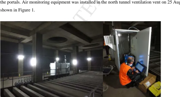
the portals. Air monitoring equipment was installed in the north tunnel ventilation vent on 25 August 2014, as is 121
shown in Figure 1. 122
123
Figure 1 – Installing measurement equipment in the CLEM7 Northbound tunnel vent. 124
M
AN
US
CR
IP
T
AC
CE
PT
ED
Air-monitoring data (five-minute average) was collected in the vent for 9 days for CO, NO, NO2, NOx, PM2.5,
125
PM10, speciated volatile organic compounds (VOCs) and polycyclic aromatic hydrocarbons (PAHs), as well as
126
variables quantifying conditions in the tunnel vent (temperature, relative and absolute humidity, atmospheric 127
pressure). 128
Nitrogen oxides (NO, NO2, NOx) were measured using a light emission (chemiluminescent) analyser (Teledyne
129
API200). Carbon monoxide (CO) was measured with an infrared absorption instrument utilising the gas filter 130
correlation technique (Teledyne API300). Particle concentrations were measured with a Thermo Scientific 1405-131
DF TEOM Continuous Dichotomous Ambient Air Monitor to simultaneously measure PM2.5 and PM10.
132
In contrast to high-resolution (5-minute) measurements of CO, NOx and PM, sampling periods for VOCs and
133
PAHs are 24 hours or longer and they were not conducted for the full measurement period. Evacuated canisters 134
fitted with timers and critical orifices were used to take VOC samples over a 24-hour period on sequential days 135
in the tunnel vent. Some canisters experienced problems with the timer and did not provide a sample. Samples 136
were successfully collected for a total of four days. The canisters were then sent for laboratory analysis using gas 137
chromatography and mass spectrometry (GC/MS) in accordance with the US EPA Compendium TO-15 analysis 138
method. PAHs have been collected using a low-volume air sampler in combination with a frit and a sorbent 139
cartridge (XAD-2 resin) over an approximately nine-day sampling period. After sampling, they were extracted 140
together to obtain the gas-phase and particle-associated PAH concentrations. Gas Chromatography – High-141
Resolution Mass Spectrometry was used for the PAHs analysis. 142
The pollutant monitoring data were checked by pre- and post-test calibration, as daily calibration for zero and 143
span values could not be carried out during the test period. Particulate matter monitoring data collected with the 144
TEOM instrument were verified according to Australian Standard AS/NZS 3580.9.13:2013. 145
Tolling statistics are continuously collected at the exit of the northbound tunnel using camera-imaging 146
technology. License plate numbers (LPNs) are collected and date-time stamped for each vehicle that passes the 147
cameras. Each vehicle is then classified as a motorcycle, car, light commercial vehicle (LCV) or heavy 148
commercial vehicle (HCV) using height, length and width of each vehicle, which are determined when the 149
vehicles travel through a specific zone on the road. Figure 2 shows the variation of traffic volumes going through 150
the tunnel by hour of day and day of the week. 151
M
AN
US
CR
IP
T
AC
CE
PT
ED
152Figure 2 – Average total traffic count by hour of day and by day of the week. 153
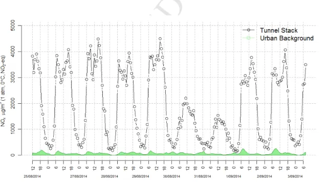
Figure 3 shows a time-series plot of measured NOx concentration levels (µg/m 3
) in the north ventilation stack, 154
including the urban background concentration levels measured at South Brisbane station. The daily variation in 155
traffic flows is clearly visible in the concentration data, as is the difference between weekdays and weekend (30 156
and 31 August). 157
158
Figure 3 – Hourly averaged tunnel vent NOx concentrations (NO2-equivalents) and urban background
159
concentrations. 160
M
AN
US
CR
IP
T
AC
CE
PT
ED
2.4 Emission computation 161Examination of five-minute data was performed to check the quality and validity of the raw concentration 162
measurements, before hourly averaged values were computed. Tunnel emissions were computed by multiplying 163
hourly-averaged measurements of time-aligned and background-corrected concentrations by tunnel air-flow data 164
(m3/h). Ambient concentration data from nearby monitoring stations were used to estimate concentrations at the 165
tunnel entrance point. Hourly vehicle travel in the tunnel is quantified with a variable called ‘vehicle kilometres 166
travelled’ (veh.km/h). Hourly VKT were computed by multiplying total traffic volume (veh/h) derived from 167
tolling statistics with total distance (km). NOx emissions were corrected for humidity.
168
2.5 In-tunnel fleet mix 169
The LPN data were cross-referenced with vehicle registration information from the Queensland Department of 170
Transport and Main Roads, and individual vehicles were allocated to one of the 226 vehicle classes used in 171
COPERT Australia. About 13% of LPN could not be matched with Queensland vehicle registration data, 172
reflecting unidentified license plates and the portion of inter-state and unregistered vehicles. A comparison 173
between the average Queensland fleet (UQ, 2014) and the in-tunnel fleet based on analysis of license plate 174
numbers revealed that there are significant differences. 175
Whereas the VKT weighted proportion of diesel and petrol/E10 vehicles is similar (~ 29% and ~70%, 176
respectively), the tunnel has higher proportion of medium passenger cars and SUVs, as compared with the 177
Queensland average fleet. Importantly, the vehicle fleet in the tunnel is substantially younger with better engine 178
and emission-control technology, as compared with the average 2010 Queensland fleet. This is partly explained 179
with the difference in base year, but also expected to reflect a tendency for newer vehicles to use tolled tunnels. 180
The impact of fleet mix on emissions is further discussed in section 3.3. 181
2.5 Road gradient and air-flow 182
In-tunnel air speeds are measured continuously and vary from 7 to 18 km/h, depending on the time of day. The 183
road gradient profile of the tunnel was determined from tunnel design maps. In-tunnel driving behaviour was 184
recorded and analysed in a brief measurement campaign of traffic conditions by driving a car in and around the 185
CLEM7 tunnel on 27 August 2014 in the morning peak hour (8:30am – 10:00am) using the ATLAS II1 smart 186
app (Safi et al., 2015). Driving behaviour in the tunnel can be characterised as ‘free-flow freeway conditions’ 187
with an 80 km/h speed limit. Using this information, the P∆P software was run to quantify the combined impact 188
1
M
AN
US
CR
IP
T
AC
CE
PT
ED
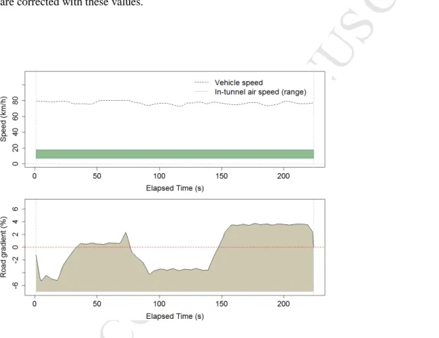
of road gradient, (piston) air-flow and tunnel driving conditions on vehicle emissions. Two input files were 189
created: 1) a second-by-second input file for in-tunnel vehicle speed, (variable) air speeds and road gradient 190
(Figure 4), and 2) a second-by-second input file with the same vehicle speed profile but with zero air speed and 191
zero road gradient (‘base case’). 192
Total emissions (grams of NOx) were then calculated for each tunnel journey for a range of in-tunnel wind
193
speeds, and divided by total tunnel distance to compute average emission factors (g/km) for LDVs and HDVs. 194
By dividing these composite emission factors with the ‘base case’ values, correction factors were computed as a 195
function of in-tunnel air speed. The results are shown in Figure 5. COPERT Australia emission factors for NOx
196
are corrected with these values. 197
198
199
Figure 4 – Visualised second-by-second input file for the P∆P software, including in-tunnel air speed (range), 200
road gradient profile and vehicle speed for tunnel. 201
M
AN
US
CR
IP
T
AC
CE
PT
ED
202Figure 5 – Correction factors for combined road grade and in-tunnel air-flow impacts on vehicle emissions in the 203
CLEM7 tunnel for LDVs and HDVs as computed with the P∆P software. 204
The road gradient effect on in-tunnel emissions is substantial with an approximately 20% net increase in NOx
205
emissions (air speed is zero km/h). However, in-tunnel air speed is predicted to have a significant impact on 206
emissions: it roughly compensates for the impacts of road gradient at higher air speeds due to reduced 207
aerodynamic drag. The average correction factor for the full measurement period, accounting for variable in-208
tunnel air-flows, is therefore small: 1.01 and 1.08 for LDVs and HDVs, respectively. 209
2.6 Start emissions 210
Cold starts contribute significantly to total vehicle emission loads, on average, 42%, 31%, 7% and 5% to total 211
emissions of CO, VOCs, NOx and PM2.5, respectively, for the Queensland fleet (UQ, 2014). The extent to which
212
in-tunnel vehicles are in cold-start mode is difficult to determine, and would require a detailed analysis of start 213
location and distance driven to the tunnel entry. This information is not readily available. However, given that 214
the bulk of cold-start emissions are typically emitted in the first minute of driving (Smit and Ntziachristos, 215
2013b) and the long length of the tunnel, it is expected that most vehicles will be driving in hot-running 216
conditions. As a result, the unknown impact of cold-start conditions is expected to be insignificant. 217
M
AN
US
CR
IP
T
AC
CE
PT
ED
2.7 High-emitters 219Vehicle ageing has a significant and unavoidable effect (increase) on vehicle emissions, and this is aggravated 220
by poor maintenance and tampering. Vehicle fleet emissions are dominated by a small percentage of ‘high-221
emitters’ with excessive emission levels, which has been confirmed by different types of emission studies 222
including laboratory test programs (e.g. Sjödin and Lenner, 1995; Pierson et al. 1999, Choo et al., 2007; RTA, 223
2009) and remote sensing studies (e.g. Zhang et al., 1995, NIWA, 2008; 2015). Studies have shown that 224
emissions from ‘high-emitting’ vehicles can be at least 50 times higher than a properly functioning catalyst car 225
(e.g. Sjödin et al., 1997), and improper maintenance (and tampering) has been indicated as the principal reason 226
for the skewness of vehicle emission distributions. The latter will remain unchecked and unverified in the 227
absence of inspection and repair programs, as is the case in Australia. 228
Recent remote sensing studies (Park et al., 2012) suggest that the skewness of (~1 Hz) emission distributions for 229
CO, hydrocarbons (HC) and NOx has increased over the last decade due to high-emitting vehicles, whereas
fleet-230
averaged emissions have decreased considerably. Bishop et al. (2012) reported that 1% of on-road vehicles in the 231
USA contributed about 10% to total vehicle emissions in the late 1980s, and that this contribution of 1% of on-232
road vehicles now has increased to about 30%. This is, to some extent, also caused by the the irregular emissions 233
behavior of modern cars, which is increasingly characterised with low emission levels and brief and large 234
emission peaks (e.g. De Haan and Keller, 2000; Smit, 2013). 235
This change in on-road emission profiles reflects two main trends 1) the penetration of cleaner vehicles into the 236
fleet over time due to increasingly strict emission standards and improved control technologies with irregular 237
emissions behaviour, and 2) the presence of vehicles that are badly tuned or have been tampered with, have 238
engine issues and/or have malfunctioning or partly functioning emission control systems (catalysts, lambda 239
sensors, faulty fuel caps, fuel injector malfunction, worn turbochargers, clogged air filters etc.). It is noted that 240
there could be other reasons for the occurrence of vehicles with excessive emission levels than tampering, engine 241
(tuning) issues and malfunctioning emission control systems, such as poorly retrofitted fuel systems and to some 242
extent even heavy loads. 243
M
AN
US
CR
IP
T
AC
CE
PT
ED
3. Results and discussion
245
3.1 NO2 to NOx ratios 246
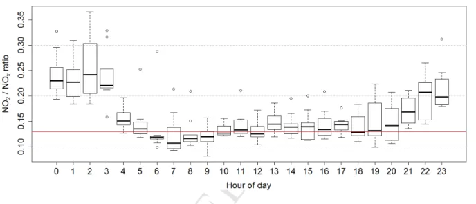
NO2 to NOx ratios are of interest as they quantify the proportion of NOx that is directly emitted as NO2. The
box-247
and-whisker plot in Figure 6 shows that NO2 to NOx ratios are typically 0.15 during times of day with significant
248
traffic volumes (6 AM – 8 PM). This is in line with expected mean primary NO2 emissions at fleet level (e.g.
249
Soltic and Weilenmann, 2003; Carslaw and Beevers, 2005). COPERT Australia predicts an average ratio of 0.13. 250
251
Figure 6 – Box-and-whisker plot of measured NO2 to NOx ratios in the tunnel by hour of day.
252
Red line shows the predicted ratio with COPERT Australia. 253
Atmospheric photo-oxidation produces ozone in the urban atmosphere, which reacts with NO in e.g. vehicle 254
exhaust producing NO2. This reaction occurs relatively fast in heavy trafficked areas, including tunnels, resulting
255
in reduced ozone concentrations and elevated NO2 concentrations (e.g. McConnell et al., 2006). At night, NOx
256
concentrations are substantially reduced (Figure 3) and ozone formation ceases. On balance, NO2 to NOx ratios
257
can be high at low ambient concentration levels (typically 0.75 to 0.90). This effect is visible in Figure 6, where 258
NO2 to NOx ratios in the tunnel are higher at night (around 0.25). At night, traffic volumes in the tunnel are small
259
(Figure 2) and ratios are more affected by ambient ratios. This suggests that for model validation, hours with 260
small traffic volumes should not be used as these measurements can be significantly impacted by potential errors 261
in estimated background concentration levels. 262
M
AN
US
CR
IP
T
AC
CE
PT
ED
3.2 Model prediction errors 264
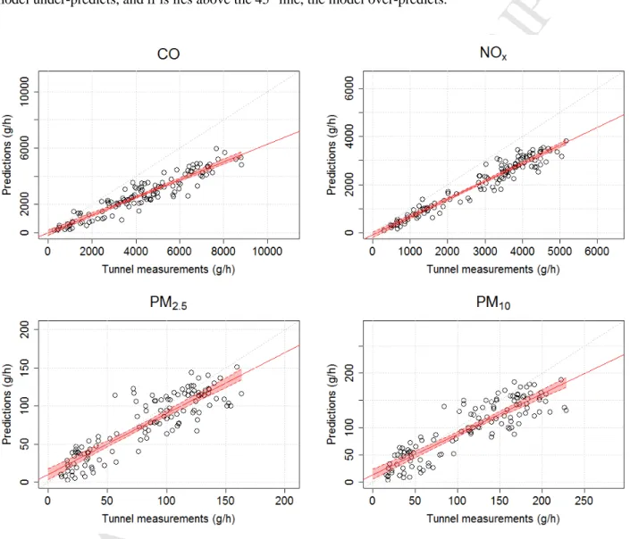
Figure 7 shows hourly emission predictions and observations in goodness-of-fit plots for each pollutant. A dot 265
point represents one hourly value. The grey dashed 45° lines indicate a perfect fit without bias. Any dot points 266
on this line show model predictions that are equivalent to observations. If a point lies below the 45° line, the 267
model under-predicts, and if is lies above the 45° line, the model over-predicts. 268
269
Figure 7 – Hourly COPERT Australia predictions versus measured tunnel emissions by pollutant (red line = 270
linear regression line, red shading = 95% confidence intervals). 271
A linear ordinary least-squares (OLS) regression model was fitted to these data: 272
= + Equation 1
M
AN
US
CR
IP
T
AC
CE
PT
ED
In this model P represents a vector of hourly predictions, O the vector of hourly observations, ββββ is a vector of 274
regression coefficients (β0, β1) and εεεε is the vector of error terms. 275
This model is useful as the slope (β1) can be used to estimate the systematic error or bias in COPERT predictions 276
in relation to the measured tunnel emissions. The coefficient of determination (R2), estimated intercept (b0) and 277
slope (b1) and bias are shown in Table 1. 278
Table 1 – Model performance statistics showing fitted regression coefficients (± standard error, p-value), 279
coefficient of determination and bias. 280 Pollutant b0 b1 R 2 Bias CO +5.66 ± 99.61 (p = 0.955) 0.63 ± 0.02 (p < 0.001) 0.88 -37% NOx -89.40 ± 56.13 (p = 0.114) 0.74 ± 0.02 (p < 0.001) 0.93 -26% PM2.5 +10.10 ± 3.61 (p = 0.006) 0.80 ± 0.04 (p < 0.001) 0.78 -7% a) PM10 +13.96 ± 4.63 (p = 0.003) 0.74 ± 0.04 (p < 0.001) 0.78 -14% b)
a bias for an average concentration value of 77 µg/m3, bias is a function of observed concentration and ranges from +52% at the lowest measured 281
concentration to –13% at the highest measured concentration, b bias for an average concentration value of 114 µg/m3, bias is a function of observed 282
concentration and ranges from +32% at the lowest measured concentration to –19% at the highest measured concentration. 283
Fitted intercepts are expected to be zero as zero emission predictions (no vehicles in the tunnel) should 284
correspond to zero emission measurements. The intercepts are not significantly different from zero for CO and 285
NOx, but are significantly different for PM. One contributing factor is that background concentration levels are
286
relatively high for PM (on average 6 µg/m3 for PM2.5 and 14 µg/m 3
for PM10). As a consequence, errors in
287
background concentration data can significantly impact on the results. There are also significant differences 288
between the empirical base for the COPERT software and the tunnel results that may significantly affect 289
measured PM mass concentrations, and can distort expected relationships with regard to traffic volume, driving 290
conditions and fleet mix. Whereas laboratory emission measurements are conducted under strictly defined and 291
controlled conditions, the tunnel PM samples measure particles that have aged (typically 8 minutes after 292
emission from exhaust pipe) and have undergone several processes such as nucleation, coalescence and 293
condensation, as well as absorption to and re-entrainment from tunnel walls. Tunnels are also uncontrolled in 294
relation to non-exhaust PM emissions, and could be significantly influenced by e.g. trucks carrying dusty loads. 295
The regression model suggests that the prediction software under-estimates emissions by 7 to 37%, depending on 296
the pollutant. These validation results appear to be relatively good. For instance, a review of 50 international 297
vehicle emission model validation studies showed that reported model prediction errors are generally within a 298
M
AN
US
CR
IP
T
AC
CE
PT
ED
factor of 2 for NOx and within a factor of 3 for CO and PM, although differences as high as a factor of 5 have
299
been reported (Smit et al. 2010). 300
A plausible factor for this consistent underestimation may be (in part) an incomplete representation in the 301
COPERT Australia emission factors of vehicles with high or even excessive emissions (‘high-emitters’), as was 302
discussed in section 2.7. This issue has been reported in other studies. For instance, NRC (2000) considered that 303
under-representation of emissions from high-emitters in the US MOBILE model was one of the chief reasons for 304
MOBILE under-predicting real-world fleet emissions. A related factor could be inaccurate computation of 305
ageing effects of Australian vehicles. Although COPERT Australia simulates the effects of ageing with generic 306
mileage-correction algorithms, they are based on limited non-Australian data. In fact, recent research suggests 307
that these correction algorithms underestimate ageing effects on emissions substantially and thus require further 308
calibration (Borken-Kleefeld and Chen, 2015). 309
3.3 Model prediction errors by vehicle class 310
Consideration of vehicle class specific prediction errors facilitates cost-effective and focused vehicle emission 311
measurement programs that target specific vehicle classes, which show substantial discrepancies between 312
observed and predicted emission factors. Composite emission factors (g/km) were computed by dividing hourly 313
tunnel emissions (g/h) by total hourly travel (veh.km/h). Hours with reduced average speeds less than 75 km/h 314
(e.g. due to tunnel maintenance) were removed to ensure homogeneous and comparable traffic conditions. 315
Hourly data with less than one vehicle going through the tunnel per minute were also removed. This is important 316
because hourly data with a small number of vehicles can be significantly influenced by errors in urban 317
background concentrations, in particular for pollutants with relatively high background levels such as particles 318
(PM), as was discussed previously. 319
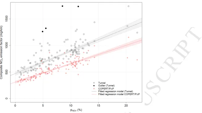
The hourly composite emission factors (e) are plotted against the percentage of heavy-duty vehicles (pHDV). An
320
example for NOx is shown in Figure 8. Figure 8 shows the hourly tunnel data, as well as the hourly predictions
321
with the COPERT Australia and P∆P model. The significant variation in the COPERT Australia and P∆P model 322
predictions reflects the impact of the changing fleet mix for each hour of the sampling period inside the tunnel. 323
M
AN
US
CR
IP
T
AC
CE
PT
ED
324Figure 8 – Measured and predicted NOx composite emission factors for each hour, fitted regression models with
325
95% prediction intervals and outliers. 326
A two-step approach was employed in the regression analysis for the tunnel data. The occurrence of excessive-327
emitters in a particular hour is expected to substantially increase the composite emission factor (g/km) and will 328
show up as outliers in the computed emission factors. It is important to include these valid outliers in the 329
determination of composite emission factors from the in-tunnel measurements. However, this poses specific 330
issues in the model-fitting process that need to be addressed. 331
Therefore a robust weighted linear modelling (RWLM) approach was first used to identify these outliers. This 332
regression is weighted with the total VKT for each hour to account for the higher accuracy of data points with 333
more vehicles. Any hourly emission value that exceeds the median value plus three times the (robust) standard 334
deviation is tagged as an outlier (shown as black solid dots in Figure 8). 335
As the second step, a (VKT-)weighted ordinary least squares (OLS) linear regression was performed on the data 336
without outliers. The regression model is defined as: 337
= + + Equation 2
338
Here eh is the mean of the hourly emission values that were tagged as outliers, and ph is the proportion of outliers
339
in the data. It is thus assumed that high-emitters 1) form a small portion of the fleet and occur randomly in time, 340
M
AN
US
CR
IP
T
AC
CE
PT
ED
and 2) are not significantly affected by the proportion of HDVs. For the CLEM7 data the number of hours with 341
outliers (significant ‘high-emitter impacts’) was 2% for PM, 3% for NOx and 4% for CO. This percentage is in
342
line with overseas reports. For instance, Choo et al. (2007) analysed 837,829 Inspection and Maintenance (I/M) 343
test results and found that approximately 4.6% of all vehicles are labelled as ‘gross polluters’. The high-emitter 344
offset (eh× ph) in equation 2 typically adds an offset value of 10-15% to the mean emission factor (pHDV = 5%).
345
A similar weighted ordinary least squares (OLS) linear regression model was fitted to the COPERT 346
Australia/P∆P model predictions (Equation 2, but without the high-emitter offset term). 347
After model fitting, light-duty and heavy-duty emission factors were computed by using pHDV values of 0% and
348
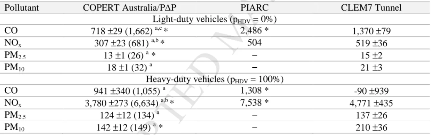
100%, respectively, in the linear regression models for each pollutant. Table 2 shows predicted and observed 349
emission factors for LDVs and HDVs, including 95% confidence limits. 350
Table 2 – Composite emission factors (mg/km) in hot-running conditions for LDVs and HDVs, including 95% 351
confidence limits and comparison with COPERT Australia/P∆P and PIARC. 352
Pollutant COPERT Australia/P∆P PIARC CLEM7 Tunnel
Light-duty vehicles (pHDV = 0%) CO 718 ±29 (1,662) a,c * 2,486 * 1,370 ±79 NOx 307 ±23 (681) a,b * 504 519 ±36 PM2.5 13 ±1 (26) a * − 15 ±2 PM10 18 ±1 (32) a − 21 ±3 Heavy-duty vehicles (pHDV = 100%) CO 941 ±340 (1,055) a 1,308 * -90 ±939 NOx 3,780 ±273 (6,634) a,b * 7,538 * 4,771 ±435 PM2.5 124 ±12 (134) a − 137 ±26 PM10 142 ±12 (149) a * − 210 ±36
a prediction for Queensland average fleet within brackets, b COPERT prediction includes P∆P correction for tunnel road gradient and air-flow, 353
c 962 mg/km if corrected for road gradient impacts, * statistically significant difference with observations (p < 0.05) 354
Table 2 shows that the fleet mix in the tunnel has a large impact on predicted emission factors. This was already 355
visible in Figure 8, which shows the variation in predictions solely due to variation in the in-tunnel fleet mix. In 356
addition, COPERT Australia predictions for the average Queensland fleet produce LDV and HDV emission 357
factors that are a factor of 1.7-2.3 and 1.1-1.7 higher, respectively, as compared with the in-tunnel fleet. These 358
results shows the sensitivity of model predictions to the local fleet mix, and indicates that detailed local fleet mix 359
information should be explicitly considered in validation studies. 360
M
AN
US
CR
IP
T
AC
CE
PT
ED
The PIARC emission factors for CO and NOx reflect the in-tunnel fleet mix and are substantially higher than
361
COPERT in all cases, varying from a factor of 1.6 to 3.5, depending on the pollutant and vehicle class. These 362
results indicate that PIARC emission factors are generally conservative. 363
In terms of prediction errors, comparison of the measured and predicted emission factors show that in several 364
cases the differences between observations and predictions are not significantly different from zero (p < 0.05), 365
i.e. PIARC: LDV NOx, COPERT Australia: HDV PM2.5, LDV PM10, HDV CO, as is shown in Table 2.
366
The PIARC and COPERT Australia CO emission factors for LDVs are 81% higher and 48% lower, respectively, 367
than the value measured in the tunnel, and these differences are statistically significant (p < 0.05). A possible 368
reason for the underestimation of CO emissions in COPERT could be additional emissions due to cold starts and 369
road gradient. The unknown impact of cold-start conditions is expected to be insignificant, as discussed in 370
section 2.6. The PIARC method suggests an increase in the CO LDV emission factor of 34% due to road 371
gradient effects in the tunnel. Correcting COPERT Australia predictions with this correction factor reduces the 372
prediction error for COPERT Australia from -48% to -30%. It is suggested that high-emitting vehicles in the on-373
road fleet and possibly inaccurate mileage correction factors play a significant role in the underestimation, as 374
will be discussed later. 375
A negative HDV emission factor is estimated for CO with the tunnel model, with a 95% confidence interval of -376
1.0 to +0.8 g/km. This large uncertainty is the result of substantial variability in observed CO emissions and 377
significant extrapolation (pHDV > 0.22). The COPERT Australia CO emission factor for HDVs is 0.9 ±0.3 g/km
378
and is not statistically significant (p < 0.05). Cold-start effects on the CO HDV emissions are expected to be 379
insignificant. The PIARC method applied to the CLEM7 tunnel suggests an increase in the CO HDV emission 380
factor of 6% due to road gradient effects. The computed PIARC CO emission factor for HDVs is about 40% 381
higher than the COPERT Australia value. 382
COPERT Australia predicts an average LDV NOx emission factor of 0.7 g/km for the Queensland fleet, but a 383
substantially lower value of 0.3 g/km for the actual fleet mix in the tunnel. These values have been corrected for 384
the impacts of road gradient and piston air-flow in the tunnel, using the P∆P software (Section 2.5). The 385
corrected LDV COPERT Australia NOx emission factor is 40% lower than the (humidity-corrected) value
386
measured in the tunnel and this difference is statistically significant (p < 0.05). This may reflect a higher-than-387
expected proportion of (diesel) vehicles with maintenance issues. The result is of interest as there is a lack of 388
empirical vehicle emissions test data for Australian light-duty diesel vehicles in particular. This is in contrast to 389
light-duty petrol vehicles for which extensive emission test programs have been carried out in Australia. As a 390
M
AN
US
CR
IP
T
AC
CE
PT
ED
consequence, European emission algorithms for diesel cars were directly used in COPERT Australia, and it is 391
the only vehicle type for which Australian vehicle emission measurements have not been available. 392
The PIARC NOx emission factor for LDVs is almost equivalent to the observed value. However, PIARC
393
overestimates the NOx emission factor for HDVs with 60% and this difference is statistically significant (p <
394
0.05). The tunnel measurements produce a composite HDV NOx emission factor of 4.7 g/km. COPERT
395
Australia predicts an average HDV NOx emission factor of 6.6 g/km for the Queensland fleet, but a substantially
396
lower value of 3.8 g/km for the actual fleet mix in the CLEM7 tunnel. These values have been corrected for the 397
impacts of road gradient and piston air-flow in the tunnel using the P∆P software. The corrected HDV COPERT 398
Australia NOx emission factor is 19% lower than the value measured in the tunnel, and the difference is
399
statistically significant (p < 0.05). This may reflect heavy-duty diesel vehicles with e.g. maintenance issues and 400
elevated NOx emissions that are not yet fully reflected in the software.
401
COPERT Australia predicts an average LDV PM2.5 and PM10 emission factor of 26 and 32 mg/km for the
402
Queensland fleet, and a substantially lower value of 13 and 18 mg/km for the actual fleet mix in the tunnel, 403
respectively. This value is about 10-15% lower than the value observed in the tunnel, but this difference is only 404
statistically significant for PM2.5 (p < 0.05). COPERT Australia predicts an average HDV PM2.5 and PM10
405
emission factor of 134 and 149 mg/km for the Queensland fleet, and a lower value of 124 and 142 mg/km for the 406
actual fleet mixes in the tunnel, respectively, which is about 10% and 30% lower than the observed values. The 407
difference is statistically significant (p < 0.05) for PM10 only. These results indicate that overall prediction errors
408
(under-estimation) for PM are small, but more significant for HDVs. Given the range of factors that complicate 409
validation for PM that were discussed before, these results show a remarkably good performance of COPERT 410
Australia. 411
The analysis of vehicle-class specific prediction errors has shown that largest prediction (%) errors for COPERT 412
Australia are observed for LDVs for the majority of pollutants (CO, NOx, PM2.5), except for PM10 where HDVs
413
have the highest (relative) error. PIARC emission factors generally show the largest prediction errors, except for 414
one very good agreement for LDV NOx. Composite emission factors in COPERT Australia are not significantly
415
different (p < 0.05) from those observed in the tunnel in 25% of the cases. COPERT Australia emission factors 416
for LDVs and HDVs have prediction errors ranging from about 10-40%. It is suggested that high-emitting 417
vehicles in the on-road fleet play a significant role in the underestimation. 418
419
3.4 VOC emission factors 420
M
AN
US
CR
IP
T
AC
CE
PT
ED
Individual hydrocarbons include gas-phase VOCs, gas-phase semi-volatile hydrocarbons (also commonly called 421
SVOCs) and particulate-phase hydrocarbons, where condensation of semi-volatile HCs on aerosols occurs. The 422
exact definition of the hydrocarbons varies in literature and depends on the measurement equipment used. VOCs 423
are roughly defined as being C1-C12 hydrocarbons, SVOCs as C10-C26 (mainly alkanes and aromatics) and
424
particulate phase hydrocarbons as C14+. Analysis of the VOC canisters identified 28 individual VOCs above the
425
limit of detection, which are mainly alkanes, alcohols and aromatics. Table 3 shows the results. 426
Table 3 – Measured and predicted emission factors (mg/km) for speciated VOCs (± standard error). 427
Speciated VOC Tunnel COPERT Australia Error
Ethanol 27.0 (±5.6) − − Acetone 15.9 (±0.9) 0.2 -99% Toluene 14.0 (±1.0) 4.7 -66% Xylene (m-& p-) 11.5 (±3.1) 3.9 -66% 2-Methylbutane 7.6 (±0.8) − − Pentane 6.1 (±0.8) 3.4 -44% Benzene 5.6 (±0.8) 2.1 -62% Methylene-chloride 4.7 (±3.6) − − 1,2,4-Trimethylbenzene 3.9 (±1.5) 1.1 -71% Hexane 3.0 (±0.6) 1.1 -62% Xylene (o-) 3.0 (±1.0) 1.9 -36% Undecane 2.6 (±1.4) 0.3 a -88% 4-Ethyltoluene 2.5 (±1.5) − − Cyclohexane 2.4 (±0.8) 0.3 b -86% p-Diethylbenzene 2.4 (±1.4) − − Decane 2.4 (±1.2) 0.2 -93% Octane 2.2 (±1.3) 0.2 -93% 1,3,5-Trimethylbenzene 2.2 (±1.2) 0.4 -83% 2,2,4-Trimethylpentane 2.2 (±1.2) − − Nonane 2.1 (±1.1) 0.1 -97% Styrene 2.0 (±1.1) 0.2 -87% Heptane 1.9 (±1.1) 0.8 -59% Ethylbenzene 1.8 (±1.0) 2.3 +24% Acrolein 1.8 (±0.1) 0.3 -85% 1,3-Butadiene 1.5 (±0.1) 0.5 -67% Isopropylalcohol 1.2 (±0.3) − − Methylethylketone (MEK) 1.0 (±0.2) 0.1 -93% Methyltert-butylether (MTBE) 0.7 (±0.0) − − ∑ ∑ ∑ ∑ 135 24
a COPERT Australia category “alkanes C
10-C12”, b COPERT Australia category “cycloalkanes” 428
M
AN
US
CR
IP
T
AC
CE
PT
ED
The difference between COPERT Australia and the tunnel measurements is large. COPERT substantially 429
underestimates emission factors for individual VOCs, typically with a factor of 5, but in some cases an order of 430
magnitude lower. 431
In addition, 43 VOCs for which COPERT Australia provides emission factors, were either not included 432
(aldehydes; 3.3 mg/km as predicted with COPERT) or were not measured above the limit of detection in the 433
tunnel. As a consequence, only 33% of the sum of speciated VOCs predicted with COPERT Australia is reported 434
in Table 3 (24 mg/km). The sum of speciated VOCs has an observed value of 135 mg/km in the tunnel, which is 435
46% lower than the total value predicted with COPERT Australia (72 mg/km). 436
The VOC profiles are quite different as shown in Figure 9. The proportion of alcohols in the observations is 437
substantial (21%) and absent in the COPERT predictions. The high observed values are related to the use of E10 438
in Queensland. The COPERT Australia VOC profile is dominated by alkanes and alkenes (47% and 17%), 439
whereas the tunnel observations have proportions of 22% and 1%, respectively. The aromatics content is more 440
similar with 36% (observed) and 29% (predicted). The observed proportion of ketones (12%) is however 441
substantially higher than the predicted value of 0.4%. 442
443
Figure 9 – Proportion of VOCs in fleet emission factors by VOC class as observed in the tunnel (“CLEM7 444
tunnel”) and the complete VOC profile as predicted with COPERT Australia (“COPERT Australia”). 445
These results demonstrate the large uncertainty in speciated VOC emission factors, and this suggests that further 446
studies to improve VOC profiles and associated emission factors are warranted. 447
448 449 450
M
AN
US
CR
IP
T
AC
CE
PT
ED
3.4 PAHs emission factors 451
Observed and predicted PAH emission factors are presented in Table 4. 452
Table 4 – Measured and predicted emission factors (ng/km) for speciated PAHs. 453
Speciated PAH Tunnel COPERT Australia Error
Napthalene 4,793,031 700,352 -85% Phenanthrene 5,264 20,841 +296% Pyrene 2,510 9,405 +275% Fluoranthene 1,377 10,625 +672% Anthracene 648 2,094 +223% Benzo(a)anthrancene 194 1,159 +497% Chrysene 194 2,599 +1,237% Benzo(e)pyrene 194 1,814 +833% Benzo(b)fluoranthene 154 1,094 +611% Benzo(g,h,i)perylene 134 1,354 +913% Benzo(a)pyrene 121 682 +462% Benzo(k)fluoranthene 81 948 +1,071% Indeno(1,2,3‐cd)pyrene 77 767 +897% Dibenzo(a,h)anthracene 49 132 +173% ∑ ∑ ∑ ∑ 4,804,028 753,869
COPERT substantially overestimates emission factors for almost all PAHs, typically with a factor of 3-13, 454
except for napthalene, which is underestimated with a factor of 7. In addition, 12 PAHs for which COPERT 455
Australia provides emission factors, were not measured above the limit of detection in the tunnel. As a 456
consequence, only 97% of the sum of PAHs predicted with COPERT Australia is reported in Table 3 (753,896 457
ng/km). The sum of PAHs has an observed value of 4.80 mg/km in the tunnel, which is 516% higher than the 458
value predicted with COPERT Australia (0.78 mg/km), and due to the discrepancy for naphtalene which makes 459
up the bulk of total PAHs. These results demonstrate the large uncertainty associated with PAH emission factors, 460
and suggests that further studies to improve PAH profiles and associated emission factors are needed. 461
462 463
M
AN
US
CR
IP
T
AC
CE
PT
ED
5. Conclusions 464This paper presents results of a tunnel emissions study that was conducted in Brisbane, Australia, to (partially) 465
validate the Australian vehicle emissions software COPERT Australia and PIARC emission factors. Emissions 466
of NOx, NO2, PM2.5, PM10, CO, VOCs and PAHs generated in the 4.8 km-long tunnel were monitored for 9 days
467
in the north ventilation vent. Other data were collected including traffic counts, license plates, in-tunnel air-flow, 468
speed-time profiles using a smart app, tunnel design maps and background concentrations. 469
Analysis found that the the in-tunnel fleet mix differs substantially from the average on-road fleet, with a larger 470
proportion SUVs and younger vehicles, leading to lower emissions by factor of about 2. 471
The P∆P software was run to examine and quantify the combined impact of road gradient, (piston) air-flow and 472
tunnel driving conditions on NOx emissions. The road gradient effect on in-tunnel emissions is substantial with
473
an approximately 20% increase in NOx emissions. However, in-tunnel air-flow roughly compensates for road
474
gradient impacts at higher air speeds due to reduced aerodynamic drag. On average, NOx emissions are increased
475
by 1-8%. 476
Typical measured in-tunnel NO2 to NOx ratios were 0.15, which is close to 0.13 predicted with COPERT
477
Australia. The results suggest that the COPERT Australia is generally accurate at fleet level for CO, NOx, PM2.5
478
and PM10, when compared with similar international studies. COPERT underestimates emissions by 7% to 37%,
479
depending on the pollutant. These findings apply only to the specific measurement conditions in the tunnel, i.e. a 480
free-flow speed of about 80 km/h, the particular road gradient profile and ventilation conditions (piston effect) 481
and the specific young fleet mix. As a consequence, these results cannot be used to make generic statements 482
about accuracy of the software. Instead, other studies are required to quantify prediction accuracy in other urban 483
conditions, using for instance remote sensing or near-road air-quality measurements. 484
COPERT Australia composite LDV/HDV hot-running emission factors for CO, NOx, PM2.5 and PM10 are not
485
significantly different (p < 0.05) from those observed in the tunnel in 25% of the cases. For the other cases, 486
emissions are consistently underestimated by ~ 10-40%, depending on the pollutant and vehicle class. The 487
largest prediction errors are observed for LDVs for the majority of pollutants (CO, NOx, PM2.5), except for PM10
488
where HDVs have the highest (relative) error. It seems plausible that three factors play a role in the 489
underestimation: 1) under-representation of high/excessive-emitting vehicles in the model due to the absence of 490
Inspection and Maintenance (I/M) programs in Australia, 2) lenient vehicle ageing (mileage) correction factors 491
in the COPERT software, and 3) lack of empirical emissions data for Australian diesel LDVs. 492
M
AN
US
CR
IP
T
AC
CE
PT
ED
Nevertheless, these validation results appear to be relatively good in comparison with other international 493
validation studies. This is particularly the case for PM, which tends to have the lowest prediction errors, despite 494
the range of factors that complicate validation for PM. In comparison with COPERT Australia, PIARC emission 495
factors are conservative and exhibit the largest prediction errors, except for one very good agreement for LDV 496
NOx.
497
In regard to speciated VOCs, the difference between COPERT Australia and the tunnel measurements is large, 498
with substantially different VOC profiles. COPERT substantially underestimates emission factors for individual 499
VOCs, typically with a factor of 5, but in some cases an order of magnitude lower. COPERT substantially 500
overestimates emission factors for almost all PAHs, typically by a factor of 3-13, except for napthalene, which is 501
underestimated with a factor of 7. These results demonstrate the large uncertainty in speciated VOC and PAH 502
emission factors, which suggests that further studies to improve local VOC and PAH profiles and associated 503
emission factors are required. 504
The results indicate that further targeted emissions testing for diesel vehicles using e.g. PEMS would benefit 505
vehicle emission modelling and air-quality assessments in Australia. Other tunnel datasets in other cities, 506
preferably of longer duration than a week, could be analysed in a similar fashion to see if these results are 507
confirmed. 508
6. Acknowledgements
509
This research did not receive any specific grant from funding agencies in the public, commercial, or not-for-510
profit sectors. 511
References
512
• Bishop, G.A., Schuchmann, B.G., Stedman, D.H., Lawson, D.R., 2012. Multispecies remote sensing 513
measurements of vehicle emissions on Sherman Way in Van Nuys, California, Journal of the Air & 514
Waste Management Association, 62 (10), 1127-1133. 515
• Borken-Kleefeld, J., Chen, Y., 2015. New emission deterioration rates for gasoline cars – results from 516
long-term measurements, Atmospheric Environment, 101, 58-64. 517
M
AN
US
CR
IP
T
AC
CE
PT
ED
• Caiazzo, F., Ashok, A., Waitz, I.A., Yim, S.H.L., Barrett, S.R.H., 2013. Air pollution and early deaths in 518
the United States. Part I: Quantifying the impact of major sectors in 2005, Atmospheric Environment, 519
79, 198–208. 520
• Carslaw, D.C., Beevers, S.D., 2005. Estimations of road vehicle primary NO2 exhaust emission fractions
521
using monitoring data in London, Atmospheric Environment, 39, 167–177. 522
• Choo, S., Shafizadeh, K., Niemeier, D., 2007. The development of a prescreening model to identify 523
failed and gross polluting vehicles, Transpn Res.-D, 12 (3), 208-218. 524
• De Fré, R., Bruynseraede, P, Kretzschmar, J.G., 1994. Air pollution measurements in traffic tunnels, 525
Environ. Health Perspect., 102, 31-37, 1994. 526
• De Haan, P., Keller, M., 2000. Emission factors for passenger cars: application of instantaneous 527
emission modeling, Atmospheric Environment 34, 4629–4638. 528
• Geller, V.D., Sardar, S.B., Phuleria, H., Fine, P.N. et al., 2005. Measurements of particle number and 529
mass concentrations and size distributions in a tunnel environment, Environmental Science & 530
Technology, 39, 8653-8663. 531
• Hausberger, S., Rodler, J., Sturm, P., Rexeis, M., 2003. Emission factors for heavy-duty vehicles and 532
validation by tunnel measurements, Atmospheric Environment, 37, 5237–5245. 533
• McConnell, R., Berhane, K., Yao, L., Lurmann, F.W., Avol, E., Peters, J.M., 2006. Predicting residential 534
ozone deficits from nearby traffic, Science of the Total Environment, 363, 166-174. 535
• Mellios, G., Smit, R., Ntziachristos, L., 2013. Evaporative emissions: developing Australian emission 536
algorithms, Proceedings of the CASANZ Conference, Sydney, 7-11 September 2013. 537
• NIWA, 2008. On-Road Vehicle Emissions Monitoring - Sydney, National Institute of Water and 538
Atmospheric Research (NIWA) Client Report: CHC2008-023, March 2008, Jeff Bluett, Prepared for 539
Department of Environment and Climate Change (New South Wales), Australia. 540
• NIWA, 2015. The Use of Remote Sensing to Enhance Motor Vehicle Emission Modelling in New 541
Zealand, Prepared by Robin Smit and Elizabeth Somervell, National Institute of Water & Atmospheric 542
M
AN
US
CR
IP
T
AC
CE
PT
ED
Research, Auckland, New Zealand. https://www.niwa.co.nz/sites/niwa.co.nz/files/AKL2015-543
012%20RSD%20evaluation.pdf 544
• NRC, 2000. Modeling Mobile-Source Emissions, National Research Council, National Academy Press, 545
Washington D.C., USA. 546
• Park, S.S., Kozawa, K., Fruin, S., Mara, S., et al., 2012. Emission factors for high-emitting vehicles 547
based on on-road measurements of individual vehicle exhaust with a mobile measurement platform, J. 548
Air & Waste Manage. Assoc, 61, 1046-1056. 549
• PIARC, 2012. Road Tunnels: Vehicle Emissions and Air Demand for Ventilation, Eds. Sturm, P., Hervé, 550
F., World Road Association (PIARC), 2012R05EN, ISBN 2 84060 269 5. 551
• Pierson, W.R., Schorran, D.E., Fujita, E.M., Sagebiel, J.C., Lawson, D.R., Tanner, R.L., 1999. 552
Assessment of nontailpipe hydrocarbon emissions from motor vehicles, J. Air & Waste Manage. Assoc., 553
49, 498-519. 554
• RTA, 2009. Second National In-Service Emissions Study (NISE2) Light Duty Petrol Vehicle Emissions 555
Testing, Roads and Traffic Authority of NSW, Report RTA.07.2828.0309, March 2009. 556
• Safi, H., Assemi, B., Mesbah, M., Ferreira, L., Hickman, M., 2015. Design and implementation of a 557
smartphone-based system for personal travel survey: case study from New Zealand, Transportation 558
Research Board 94th Annual Meeting, Washington DC, US. 559
• Soltic, P., Weilenmann, M., 2003. NO2/NO emissions of gasoline passenger cars and light-duty trucks
560
with Euro-2 emission standard, Atmospheric Environment, 37, 5207–5216. 561
• Sjödin, Å, Andréasson, K., Wallin, M., Lenner, M., Wilhelmsson, H., 1997. Identification of high-562
emitting catalyst cars on the road by means of remote sensing, Int. J. of Vehicle Design, 18 (3/4), 326-563
339. 564
• Sjödin, Å., Lenner, M., 1995. On-road measurements of single vehicle pollutant emissions, speed and 565
acceleration for large fleets of vehicles in different traffic environment, The Science of the Total 566
Environment, 169, 157-165. 567
M
AN
US
CR
IP
T
AC
CE
PT
ED
• Smit, R., Brown, A.L., Chan, Y.C., 2008. Do air pollution emissions and fuel consumption models for 568
roadways include the effects of congestion in the roadway traffic flow?, Environmental Modelling & 569
Software, 23 (10), 1262-1270. 570
• Smit, R., McBroom, J., 2009. Use of overseas emission models to predict traffic emissions in urban 571
areas - Technical Note, Road and Transport Research, 18 (3), 52-60. 572
• Smit, R., Ntziachristos, L, Boulter, P., 2010. Validation of road vehicle and traffic emission models — a 573
review and meta-analysis, Atmospheric Environment, 44 (25), 2943-2953. 574
• Smit, R., 2013. Development and performance of a new vehicle emissions and fuel consumption 575
software (P∆P) with a high resolution in time and space, Atmospheric Pollution Research, 4, 336-345. 576
• Smit, R., Ntziachristos, L., 2013a. COPERT Australia: a new software to estimate vehicle emissions in 577
Australia, Australasian Transport Research Forum 2013 Proceedings, 2 - 4 October 2013, Brisbane, 578
Australia. 579
• Smit, R., Ntziachristos, L., 2013b. Cold start emission modelling for the Australian petrol fleet, Air 580
Quality and Climate Change, 47 (3). 581
• Smit, R., 2014. P∆P: A simulation tool for vehicle emissions and fuel consumption software with a high 582
resolution in time and space, Vehicle Technology Engineer, SAE Australasia, July 2014, 17-21. 583
• UQ, 2014, Australian Motor Vehicle Emission Inventory for the National Pollutant Inventory (NPI), 584
prepared by Robin Smit, University of Queensland, Project C01772, 2 August 2014, 585
http://www.npi.gov.au/resource/australian-motorvehicle-emission-inventory-national-pollutant-586
inventory-npi. 587
• Zhang, Y., Stedman, D.H., Bishop, G.A., Guenther, P.L., et al., 1995. Worldwide on-road vehicle 588
exhaust emissions study by remote sensing, Environ. Sci. Technol., 29, 9, 2286-22. 589