Performance Reduction For Automatic Development of Parallel Applications For Reconfigurable Computer Systems

Performance Reduction for Automatic Development

of Parallel Applications for Reconfigurable Computer Systems

c

The Authors 2020. This paper is published with open access at SuperFri.org

In the paper, we review a suboptimal methodology of mapping of a task information graph on the architecture of a reconfigurable computer system. Using performance reduction methods, we can solve computational problems which need hardware costs exceeding the available hardware resource. We proved theorems, concerning properties of sequential reductions. In our case, we have the following types of reduction such as the reduction by number of basic subgraphs, by number of computing devices, and by data width. On the base of the proved theorems and corollaries, we developed the methodology of reduction transformations of a task information graph for its automatic adaptation to the architecture of a reconfigurable computer system. We estimated the maximum number of transformations, which, according to the suggested methodology, are needed for balanced reduction of the performance and hardware costs of applications for reconfigurable computer systems.

Keywords: performance reduction, hardware costs, reconfigurable computer system, parallel applications development, information graph.

Introduction

Most researchers of parallel computing [1–4] admit that parallel programming is a complex area. It is necessary to organize and control a large number of processes that asynchronously run on the nodes of a multiprocessor computer system (MCS). The demanding requirements are decreasing of the calculation time and increasing of the results accuracy. To fulfill these requirements, we increase the number of nodes of a multiprocessor computer system, but at the same time, development of parallel programs becomes more complex.

For a long time, we believed that it is possible to cope with the growing complexity of parallel program development with the help of automatic parallelization of sequential processor (procedural) programs. In this case, a parallelizing compiler [1, 2, 5–10] receives an imperative processor program, reconstructs the natural parallel structure of its initial algorithm, detects its fragments for concurrent execution (e.g. loop iterations suitable for parallelization), and adds all necessary instructions. However, the automatic parallelization of sequential programs is a computationally expensive problem with an extremely large number of variants for analysis.

The parallelizing compiler has to analyze different variants of multiple fragments of the procedural program. At the same time, it analyses distribution of data among the nodes of the multiprocessor computer system according to its switching network. These two reasons complicate automatic parallelization for clusters that are the most widely used multiprocessor computer systems with distributed memory.

Let us have a cluster computer system, which consists ofnnodes, and each node processes its local part of data. In this case, we describe the data distribution among the nodes using ann-ary tree. According to the Cayley theorem, we estimate the number of variants of data distribution as the number of different trees for n vertices, i.e.nn−2. For example, the cluster MCS consists of 64 nodes. So, the number of possible distribution variants is 6462= 2372. Analysis of such num-ber of variants on any existing computer system and during any reasonable time is impossible.

Therefore, the most part of research in this problem domain was devoted to heuristic methods of search space reduction (e.g. the analysis of information dependencies [1], loop nests and it-erations [4–6], private and reduction variables [7, 8], canonization, loop unrolling/unwinding, loop fusion, loop distribution [9, 10], etc.). Formal transformations and heuristic methods, de-veloped for rejection of inefficient parallel program variants [3], require some recommendations and instructions given by the programmer; otherwise, they cannot provide efficient automatic parallelization of any procedural program.

Nowadays, multi-chip reconfigurable computer systems (RCS) [11] with field-programmable gate arrays (FPGAs) are widely used for solving of computationally expensive problems in various fields of science and technology. RCSs contain multiple FPGAs of a large logical capacity. The FPGAs are connected by a spatial switching system into a single computational field. Within such computational field, we implement calculations as a computing structure [12–14] and decrease the solution time [15, 16] by one or two orders of magnitude at the considerably lower (by a factor of 6–8) processing rate. For certain problem domains [17, 18], RCSs are considerably superior in real performance and power efficiency in contrast with cluster MCSs.

In the paper, we consider a theory which helps to reduce the number of variants parallel calculations for analysis and further synthesis of a computing structure for an RCS. We represent a task as an information graph and then, using performance reduction methods and a relatively small number of steps, we transform it into the form, similar to the architecture of an RCS. For most applications, it is possible to synthesize computing structures and to increase the task solution time owing to the performance reduction methods. In this case, the efficiency of the designed structures is not less than 50 % in comparison with those designed by circuit engineers. Let us review the structure of the paper. In the first section we describe the forms of parallel calculations, and the task information graph used for structural and procedural calculations on the RCS. In the second section, we consider performance reduction as a way of implementing of the task information graph on the RCS with the lack of its hardware resource. In the third section, we represent the performance reduction methods for decreasing of hardware costs, required for implementing of the information graph, and prove theorems on the applicability of reduction transformations. In the fourth section, we represent the performance reduction principles for mapping of the task information graph on the RCS architecture. Besides, here we estimate the number of computing structures that are to be analysed for adaptation of the initial task information graph to the architecture and hardware resource of the RCS. In the fifth section, we describe the rules, according to which we use the reduction transformations in an experiment for verification of our performance reduction methods. The rules were used in tools for parallel application development. In the conclusion we generalize our results and discuss the directions of our future research.

1. Forms of Calculations

When we represent calculations as a graph, we describe a task or its fragment in an abso-lutely parallel form, i.e. as an acyclic oriented graph with input, output, and operation vertices connected by arcs according to the data processing order (but not according to the control transfer). There are various forms of graph models for computational tasks such as algorithm graphs [1], information graphs [1, 19], dependency and influence graphs, and lattice graphs [1]. Arcs of a graph show, how arguments of operation vertices depend on results of calculations, performed by other operation vertices, or arguments, received from input vertices. This is an information connection (or information dependence) that describes relations between two ver-tices of a graph when the output argument of each vertex is the input of another one. If we speak about multiprocessor architectures [1], then information dependence between two oper-ators means addressing to the same memory cell during their execution. If we speak about dataflow architectures, then it means addressing to one and the same element of a flow.

The most common forms are an algorithm graph [1] and an information graph [1, 19]. The algorithm graph describes a computational task as a set of simple operations (addition, multiplication, division, etc.) distributed into levels. Although, it is possible to use complex composite operations (macro operations) as level vertices [1]. All vertices of the algorithm graph, represented in the canonical parallel form, are distributed into numbered subsets, which form levels. Here, the first vertex of each arc belongs to the level, whose number is less than the number of the level, which contains the last vertex. Besides, arcs cannot connect vertices which belong to the same level.

The theory of structural and procedural calculations [19] deals with a task information graph (TIG). In contrast to the parallel forms of an algorithm graph, the task information graph is a combination of layers and iterations. A layer consists of isomorphic, functionally complete, and information independent subgraphs of a task instead of operation vertices. Iterations describe dependencies among processing data over time without considering latency. Subgraphs from one and the same layer are information independent, i.e. not connected by arcs. Subgraphs, which belong to different iterations, depend on processing data. The number of isomorphic subgraphs in a layer is similar to the level width of the canonical parallel form, and the number of iterations is similar to its height, if we consider isomorphic subgraphs as macro-operations. In comparison with an algorithm graph, a TIG describes a task at a higher level of hierarchy. In this case, we use separate operations, but subgraphs which consist of several operations. The information graph describes the absolutely parallel form of the task. The task parameters define the number of iterations. Therefore, the TIG has no dataflows.

A structural implementation of a TIG on a computer system provides the highest perfor-mance. In this case, the number of devices is equal to the number of operation vertices (or operations) of a solving task, and the number of input/output arcs is equal to the number of external memory channels. For the majority of applications, such structural implementation of a TIG is impossible, because the number of devices and channels in any RCS is limited. Therefore, if we map a TIG on a real RCS with its limited hardware resource, we transform this TIG into a computing structure with the lower performance and lower requirements for the number of channels, the number of concurrently functioning devices, and/or the data width in comparison with the structural implementation of this TIG.

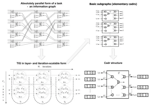
Figure 1. Transformation of a TIG into the computational structure via layer- and iteration-scalable form

interval, clock rate, etc. We assume, that the term “implementation of a subgraph on a computer system” means a computing structure which consists of hardware-programmed devices with timing characteristics (or so-called timing component).

Figure 1 shows the transformation a TIG for its structural implementation on an RCS. To transform the absolutely parallel form of a TIG into the layer- and iteration-scalable form, we obtain the functionally regular form [19] with functions of layer mapping between iterations Φi, and functions of isomorphic subgraph ordering in a layer Fij:

G= Φ(Fij(gij)), (1)

where gij is a basic subgraph (a pipeline computing structure); Fij is an ordering function

for information-independent subgraphs in a computational layer; Φi is a mapping function of

information-dependent layers. The composition of functionsFij and Φi depends on an available

RCS hardware resource ARCS.

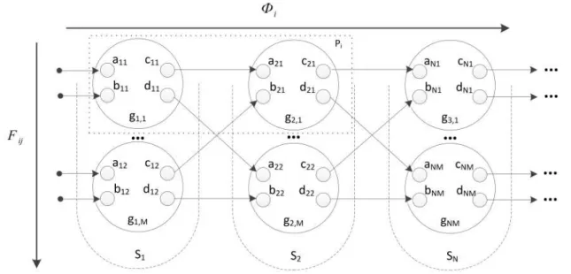
Figure 2 shows the task information graph, which consists of information-dependent layers S1, ..., SN. Each layer consists of isomorphic information-independent subgraphs G1,1, ..., G1,M, ...GN,M.

Owing to such form, we easily scale the task computing structure. If we change the number of basic subgraphsgij in the composition of the functionsFij and Φi, then we scale the computing

Figure 2.The information graph, its layersFij and iterations Φi

A basic subgraphgij is a minimal indivisible element of a task. When its computing structure

is mapped on an RCS, it is completed with functions of reading, writing, and recursion, derived from Fij and Φi functions. The obtained indivisible program structure is called a cadr. For all

obtained cadrs we specify an order relation, which, together with the von-Neumann determinism, define the execution sequence of cadrs according to their control program.

A basic subgraph is a functionally completed fragment of a TIG. It consists of subgraphs of one or several subtasks. It is possible to map any basic subgraph on an available RCS hard-ware resource. Completed with the synthesized read/write functions, a basic subgraph provides solution of a task. Within the theory of structural and procedural calculations, basic subgraphs are selected according to available hardware resource. In this case, selection criteria are not formalized; they are determined by the structure of a task, by available resource, and by the developers experience. To select a basic subgraph, the developer analyzes the TIG and looks for frequently used fragments of the TIG which are typical for a certain problem area. Here are the examples of such frequently used fragments:

• addition, multiplication, and division of matrix elements (linear algebra);

• calculations in mesh points (mathematical physics);

• round transformations with logical “AND”, “OR”, “exclusive OR”, and fixed-size data block offset (symbolic processing);

• the discrete fast Fourier transform operation (digital image and signal processing). Usually, these standard fragments form basic subgraphs of various tasks. We can select basic subgraphs in procedural programs, using descriptions of loops, because fragments with cyclic processing correspond to functional subgraphs, i.e. to calculations with specified scaling functions by layers Fij and by iterations Φi. Here, the operators of a loop body are a basic subgraph.

Information dependencies among operators, and cycle description determine the functions of layers Fij and by iterations Φi. As a rule, any basic subgraph consists of multiple functional

2. Mapping of Information Graphs on Reconfigurable

Computer Systems

The available hardware resource ARCS defines not only mapping functions Fij and Φi, but

also the calculations of the basic subgraph. That is why, we can represent (1) as

G(ARCS) = Φpar ARCS

◦ Φpipe(Fpar ARCS

◦ Fpipe(gstr ARCS

◦ gproc)), (2)

where “par” and “pipe” mean parallel and pipeline execution, respectively; gstr is the

struc-tural form of the basic subgraph; gproc is the procedural form of the basic subgraph; ARCS

◦ is composition of scaling functions, which depends on the available hardware resource ARCS.

Using the dependence between the basic subgraph and the available hardware resource (2), we can describe not only extreme variants of completely structural (gstr) and completely

proce-dural (gproc) calculations, but other intermediate ones. However, we cannot obtain the structural

form gstr for some tasks due to hardware resource limitations, and the procedural form cannot

provide results of adequate accuracy in reasonable time. The examples of such tasks are:

• molecular simulation (docking of inhibitors);

• synthesis of new chemical compounds;

• 3D simulation of spatial physical processes (e.g. tomography of the Earth surface);

• high-resolution simulation of physical processes;

• symbolic processing, etc.

Tasks with variable data flow density [20] belong to this type also. For such tasks, the amount of processed data in various TIG subtasks may differ by 2–4 decimal places, and may depend on input data. For such tasks, basic subgraphs from different layers are significantly non isomorphic. If we try to transform them into isomorphic subgraphs, using the union operation, then we need an inaccessible hardware resource for their structural (or structural-procedural) variant. Hence, we cannot solve these tasks using structural, structural-procedural, or procedural calculations.

If we want to solve these tasks during some reasonable time and using some available hard-ware resource, it is necessary to reduce the hardhard-ware costs for gstr, not using the completely

procedural variantgproc, in order to create the basic subgraph within an RCS, and to provide the

specified task performance. Here, the task performance is lower than the one for the structural variant gstr, but higher than the one for the procedural variantgproc.

Therefore, we consider a basic subgraph as a scalable, not an atomic object of a task. If we reduce the performance and hardware costs, then it is possible to fulfill all requirements of the task and solve it.

For the first time [20], it was suggested to use performance reduction methods for decreasing of hardware costs in case, when RCS hardware resource is insufficient for even one basic sub-graph. The main effect of performance reduction is a linear increase of the task solution time, proportional to the reduction coefficient. The main reduction transformations, which provided balanced scaling of molecular docking tasks in [20], are the following:

• RN _{– the reduction by number of basic subgraphs. It decreases the number of computing}

structures, simultaneously mapped on RCS.

• ROp _{– the reduction by number of computing devices. It decreases the number of}

types are combined in one device. Besides, new connections for operands synchronizations are synthesized.

• Rρ_{– the reduction by data width. It decreases the number of concurrently processed digits.}

Absolutely parallel processing of digits in each operand is transformed in partly parallel or sequential processing.

• RS – the reduction by data processing interval. It increases the data processing/supply in-terval; the hardware costs remain unchanged. This type of reduction is used for matching of data flow with different density among different subtasks or information graph fragments.

• RF req – the reduction by clock rate. It decreases the clock rate of a computing structure, which implements some information graph fragment, and matches data flows with different density.

In [20], all reduction transformations were used to reduce hardware costs for solution of some task. However, we can consider the methods of performance reduction as transformations, which provide scaling of a TIG as a computing structure for further mapping on RCS architec-ture. Moreover, we often use the reduction transformations to get a computing structure from the absolutely parallel form of a task. As a result, the performance of the obtained computing structure is lower, but the structure requires less number of channels and simultaneously oper-ating devices, and/or less data width. That is why we may consider the computing structure of a TIG, mapped on RCS architecture, as performance reduction. Of course, this is true only in case, when RCS hardware resource is insufficient for task solution.

We efficiently use the methods of performance and hardware costs reduction for information graph mapping on RCS architectures. These methods provide automatic (without the program-mers instructions) adaptation of applications to various RCS architectures, and solve the problem of application portability.

3. Methods of Performance and Hardware Costs Reduction

The task solution performance is a number of computing operations performed per time unit during execution of an application. Let us have a computing structure F with NF basic

subgraphs. Each basic subgraph contains OpF computing devices, which process data of a ρF

width. The total number N CF of computing operations, required for processing of a data flow

with a length N, is

N CF =N ·NF ·OpF ·ρF. (3)

The task solution time for a computing device with a clock periodτ = 1/F req and with an interval S is t= N ·S·τ. Here, the data processing interval is measured in cycles. Then, the performance of the computing structure F is defined as

P erfF = N CF

t =

N_·NF ·OpF ·ρF N ·S·τ =

NF ·OpF ·ρF

S·τ =

NF ·OpF ·ρF ·F req

S . (4)

If we carry out the performance reduction with the integer reduction coefficientR, then the performance (2) is reduced by R times:

P erfF(R) =

P erfF

R =

NF ·OpF ·ρF S·τ ·R =

NF ·OpF ·ρF ·F req

S·R . (5)

for their switching and synchronization are multiply scaled. Concerning (5), it means that the cofactors of the numerator are reduced by the reduction coefficientR(or by its prime cofactors). According to (5), we can reduce the performance of a task computing structure by:

• decreasing of the number NF of hardware-programmed basic subgraphs in proportion to R (or its prime cofactors). For each mapped BS, the length N of its processed data flow increases. This method is traditional for scalable calculations, performed on RCS and clusters;

• reducing of the number OpF of computing devices in the task basic subgraph [20] in

proportion to R(or its prime cofactors). The number of operations, performed by each computing device, and the number of data processing cycles increase. This method is used for RCS;

• decreasing of the processed data width ρF in proportion to R (or its prime cofactors).

The method is used for fixed-point data, and used with restrictions for floating-point data. The number of processing cycles multiply increases. At the same time, the number of data processing channels multiply decreases. This reduction is used in case of lack of input data channels (the most typical case for RCS);

• increasing of the data processing interval S;

• decreasing of the clock rateF req [20].

In the first, second, and third cases, we reduce both the performance and the hardware costs for the computing structure F, if the switching and synchronization costs do not exceed the reduced resources. If we use the two last methods, we only reduce the performance of a task or its fragment. In this case, the hardware costs remain unchanged. We can use these methods for matching of data processing rates in different task fragments.

So, we reduce the hardware costs and the number of RCS channels, needed for the computing structure F, only if the hardware costs for switching and synchronization do not exceed the reduced resources.

The performance reduction methods without hardware costs reduction are the following:

• the reduction by clock rate;

• the reduction by data processing interval.

A multiple integer, unified for all task fragments automatic performance reduction (5) pro-vides a balanced computing structure. Thus, all task fragments are to be reduced not only with the same reduction coefficient R, but the types and coefficients of performed reductions are to be the same. However, for real tasks such requirement is almost impossible.

If we reduce the performance in order to decrease the hardware costs, then all types of reduction transformations are performed in a balanced manner. Here, the reduction coefficient is a positive integer not less than unity. Owing to the reduced computing structure, we can solve the task on lesser hardware resource with longer solution time (in proportion to the reduction coefficient).

In order to describe all reductions of the modifying computing structure, we suggest to use an operation, which rounds rational numbers down to unity [21]. For natural numbers a _≥ 1 and b_≥1, the operation is defined as

a b

1

=

  

adivb, a > b,

where div is integer division; _{b c}1 is similar to the standard floor notation b c [21], and it

indicates that the result of the “floor” operation is bounded below by unity.

The result of the floor operation _{b c}1 corresponds to the physical meaning of the

param-eters that are being reduced, because the number of basic subgraphs, computing devices, and processed digits cannot be less than unity after the reduction. The traditional “floor” operation

b c has a useful property given in [21]. For the real numbers m,x and the natural number n

x m n = x m_·n

. (7)

Since the set of natural numbers is a subset of the set of real numbers, and function (4) is monotonic and continuous, equality (7) is valid for the proposed function, too. Taking into account the commutative law, we obtain:

x m 1 n 1 = x n 1 m 1 = x m_·n

1

. (8)

Taking into account (8), we prove the following important theorem, which represents the reduction coefficient as a production of coefficients for the sequential reduction transformation. We denote sequential reduction by _×.

For example, the sequential reductions by number of basic subgraphs and by number of computing devices we represent as RT

n ×RTOp =Rn·m. Theorem 1.

Sequential T-type reductions RT

mand RTn with natural coefficients m > 1 and n > 1 are

equivalent to the reduction RT

n·m of the same type with a coefficient (m·n)>1:

R_nT _×RT_m=RT_n·m. (9)

Proof.LetF be a task fragment which contains NF basic subgraphs. Each basic subgraph

contains OpF computing devices and processes data with a width ρF. The total amount of

calculationsN CF inF is

N CF =NF ·OpF ·ρF. (10)

Since reduction transformations are independent, then we prove (9) for each type of reduc-tion.

Let us prove condition (9) for the reductionRN

n by the number of basic subgraphs with the

reduction coefficientn. The number of basic subgraphs inF is reduced to_bNF

n c1, and the total

amount of calculations N CN n is:

N C_nN =

NF n

1

·OpF ·ρF. (11)

The sequential reductionRN_m of the same fragment providesm-fold decreasing of its number of basic subgraphs. According to (8), we transform (11) and obtain

N C_nN_××_mN =

bNF n c1 m

1

·OpF ·ρF =

NF n_·m

1

·OpF ·ρF. (12)

The total amount of calculations (12), which we obtain as results of the sequential reductions by number of basic subgraphs with the coefficientsnandm, and as results of the reductionRN

by number of basic subgraphs with n_·m instead of n in (11), have the same value. This fact proves Theorem 1. In a similar way, we prove (9) for the reduction by number of computing devices, and for the reduction by data width. As a result, we prove Theorem 1 in general.

Let us formulate several corollaries for application of reduction transformations.

Corollary 1.1 of Theorem 1. Using factorization of performance reduction coefficients, we decrease the number of steps, required for selection of reasonable coefficients for sequential reductions of the same or different types. Besides, for the specified reduction coefficient we choose the best suited type of reduction transformations according to the parameters of a solving task. If the performance reduction coefficientRis a prime number, which exceeds 2, and if we cannot obtain it by a single reduction, then it is reasonable to perform not an R-fold, but an (R+ 1)-fold reduction. In this case, we obtain fully R times lower hardware costs. Since (R + 1) is an even composite number, we sequentially perform reduction transformations with reduction coefficients taken from the prime factorization of (R+ 1).

Corollary 1.2 of Theorem 1. There is no need to return to the initial basic subgraph, when the reduction coefficient multiply increases during sequential reduction of one and the same. If the result of a reduction transformation is a computing structure, which requires additional multiple (not less than twofold) decreasing of hardware costs, and its reduction type permits multiple increasing of its coefficient, then, according to Theorem 1, sequential reduction with no return to the initial basic subgraph lessen the number of steps to get a final reduced structure. According to Theorem 1, Corollaries 1.1 and 1.2, the total coefficient of sequential reductions equals to a product, but not to an algebraic sum of reduction coefficients. Therefore, it is impossible to get a reduced computing structure with a coefficient from a structure with a coefficient (n + 1) using sequential reductions of any type. Let us prove this statement (or Theorem 2) more strictly for a generalized case with a reduction coefficient (n+x).

Theorem 2.

In the general case, for a basic subgraph reduced with a coefficient n, we cannot obtain a computing structure with a reduction coefficient (n+x) for a prescribed x≥1, using sequential reductions of a type T with a natural coefficientk >1:

RT_n1×RT_k2 6=R_n+xT . (13)

Proof.According to Theorem 1, it is possible to fulfil (13) for reductions of the same type

T only if

n_·k=n+x (14)

is valid.

Then, we transform (14) and obtain

k= 1 +x

n. (15)

According to Theorem 2, the numbersn,kandxare positive integers. So, we solve (15) for

k only whenx is integrally divided by n, but not_∀x_≥1. This fact proves Theorem 2.

If we perform reductions of different types, then the similar computing structures from the left and right sides of (13) have the same total amount of operations

Therefore,

N C n_·x

1

=

N C n+x

1

, (17)

which requires

n_·k_≥n+x and n+x_≥n_·k (18)

to be fulfilled.

Both conditions are true only if

n_·k=n+x. (19)

So,

k= 1 +x

n. (20)

Under hypothesis of Theorem 2,n,k, andxare positive integers. Hence, the solution of (20) for k is possible in the natural domain only when x is integrally divisible by n, but not when

∀x_≥1. This conclusion leads to contradiction and, as a result, proves Theorem 2.

Using Theorem 2, we formulate a corollary which is important for application of a sequence of reduction transformations.

Corollary 2.1 of Theorem 2. For a reduced structure, it is impossible to increase the reduction coefficient by an arbitrary value, performing sequential reductions of any types. Hence, in general case, if additional reduction (of hardware costs) is needed, we return to the initial basic subgraph and perform reduction transformations again with a new (increased) reduction coefficient R. As a result, we need more steps to obtain the reduced computing structure.

Let us analyse, how a sequence of reduction transformations of various types influences on a final computing structure.

Theorem 3.

The superposition of reductions of different types (e.g. a reduction T1 with a coefficient n, and a reduction T2 with a coefficient m) is commutative. Therefore, if we change the order of reductions of different types for a task fragment, then the result information graph of the fragment remains unchanged:

RT_n1_×RT_m2 =RT_m2_×RT_n1,

where T1 and T2 are the types of reduction transformations; nand m are the reduction

coeffi-cients.

Proof.Let us prove commutativity of sequential reductions. The first reduction is performed by number of basic subgraphs, and the second one – by number of computing devices:

RN_{n ×}ROp_m =ROp_{m ×}RN_n. (21)

After the reduction RN

n, which is performed by number of basic subgraphs and has the

reduction coefficientn, the total amount of calculations N CN

n over binary digit bits is

N C_nN =

NF n

1

·OpF ·ρF. (22)

devices with the coefficient m decreases only the number of devices, and the total amount of calculations over binary digit bits is

N C_nN_××_mOp =

NF n

1

·

OpF m

1

·ρF. (23)

For the right side of (21), the sequential reductions ROpm and RNn lead to the same total

amount of calculations over binary digit bits:

N C_mOp_××_nN =

NF n

1

·

OpF m

1

·ρF. (24)

We prove commutativity for all other possible combinations of sequential reductions in the same way. As a result, this fact proves Theorem 3.

Using Theorem 3, we define a corollary for estimation of the number of reduction steps.

Corollary 3.1 of Theorem 3. If the order of reduction transformations is changed, it is not necessary to return to the initial basic subgraph in order to decrease the number of steps.

4. Performance Reduction Methods for Information Graphs

Mapping on Reconfigurable Architectures

Taking into account the proved theorems and corollaries, let us formulate the main rules information graph adaptation to RCS architectures.

1) To decrease the number of steps of reduction transformations, it is reasonable to choose coefficients of each type of reduction from the prime factorization of the reduction coefficient.

2) If the number of basic subgraphs in an information graph is more than 1, then it is reasonable to perform the reduction by number of basic subgraphs as the first step of reduction transformations.

In this case, we linearly decrease the required hardware resource such as the number of FPGA logic cells, and the number of channels for data parallelization.

3) If we perform the reduction by number of computing devices, and by data width to decrease the number of steps of reduction transformations, it is reasonable to perform reductions of each type until the value, specified by reduction criteria, is reached. After that, we perform reduction of another type. Here, the value is chosen according to the cofactors of the reduction coefficient of an information graph.

In this case, we reduce additional overhead of switching hardware.

Owing to the performance reduction methods, which we use for information graphs mapping on RCS architectures, it is possible to divide the set of parallelization variants into several classes that consist of isomorphic computing structures. As a result, we have few variants for analysis. Let us estimate the number of steps of reduction transformations, which we need to adapt an information graph to a reconfigurable architecture. We consider the most general case, when it is necessary to perform all types of reduction transformations (by number of basic subgraphs, by number of computing devices, and by data width) for reduction of hardware costs.

To define the initial value of a performance reduction coefficientRof a computing structure, we use its approximate value the coefficient of necessary hardware costs reductionRT, defined

as a proportion of the hardware resource, needed for hardware-programmed information graph, to the available RCS resource ARCS. The hardware resource AT for hardware-programmed

component of an FPGA (the number of Look-UP Tables (LUTs), Memory LUTs (MLUTs), Flip-Flops (FFs), the number of Digital signal processor blocks (DSPs) and Block RAM (BRAMs)). For an RCS we use the parameters of FPGA chips as follows:

AT ={ALU T_T , AM LU T_T , AF F_T , ADSP_T , ABRAM_T },

ARCS ={ALU TRCS, AM LU TRCS , AF FRCS, ADSPRCS, ABRAMRCS }. (25)

A hardware costs reduction coefficient for each resource is a proportion of the hardware costs, needed for task solution, to the available resource. We select the task hardware costs reduction coefficient as the maximum value among the calculated values:

RT =M ax( ALU T

T ALU T_RCS,

AM LU T T AM LU T_RCS ,

AF F T AF F_RCS,

ADSP T ADSP_RCS,

ABRAM T

ABRAM_RCS ). (26)

The initial value of the performance reduction coefficient R0 is equal to the coefficient RT,

rounded up to the nearest integer: R0 =dRTe.

For linear and iterative computing structures, used in tasks of symbolic processing and linear algebra, respectively, the hardware costs reduction coefficientRT and the performance reduction

coefficientR0 can be the same. In most cases, it turns out that for performance reduction with a

coefficient, which is equal to the hardware costs reduction coefficient, it is necessary to increase the performance reduction coefficient even more, due to unforeseen switching costs. Since the overall reduction coefficient is nonadditive for sequential reduction (according to Theorem 2), then it is necessary to increment R0 by 1, and to perform reduction with a new coefficient.

Performance reduction is carried out for the initial value of the performance reduction coeffi-cientR0>1, which, according to the fundamental theorem of arithmetic, and to Corollaries 1.1

and 3.1, is a product of prime cofactors:

R0=Y

i

r0i. (27)

To perform reduction transformations, taking into account the task parameters, and the prime factorization of the reduction coefficient R0, we represent it as a product of three

coeffi-cients of reduction transformations:

R0 =R₀N·ROp₀ ·R₀ρ. (28)

IfR0 is a prime number, we increment it by 1 according to Corollary 1.1.

Since in our case all reductions are performed, then all reduction coefficientsRN₀ (by number of basic subgraphs),ROp₀ (by number of computing devices) andRρ₀(by data width) exceed unity. In the first step, it is reasonable to perform the performance reduction by number of basic subgraphs with the coefficientRN

0 . In the second step, we perform the reduction by number of

computing devices with the coefficientROp₀ . The extreme case of subgraph reduction by number of computing devices means sequential execution of its operations as gproc (2) in one device

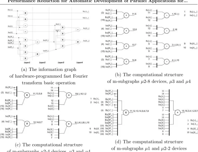
Let us consider reduction by number of devices for a basic operation of the fast Fourier transform with calculation of coefficients. Its information graph contains 16 operations such as 8 multipliers, 4 adders, and 4 subtractors (see Fig. 3a). Taking into account, that hardware-programmed addition and subtraction are identical, we claim that 8 multipliers and 8 adders are enough for the hardware-programmed information graph.

In the case of reduction by number of devices for a basic operation of the fast Fourier transform it is possible to suggest not less than 5 different variants called m-subgraphs. Each m-subgraph is characterized by its own data processing interval and hardware costs:

1. An m-subgraph µ1 (minimal, Fig. 3d) contains not more than one device for each type of

the operations of the subgraph. For our example, µ1 contains 2 devices – a multiplier and

an adder.

2. An m-subgraph µ2 (multiple) represents a multiple reducing of the number of devices in

the subgraph, and is similar to factoring out. Several variants of µ2 are possible, such as

8 devices (4 multipliers, 4 adders, Fig. 3b), 4 devices (2 multipliers, 2 adders, Fig. 3c), and 2 devices (1 multiplier, 1 adder, Fig. 3d).

3. An m-subgraph µ3 contains all devices from a layer with the maximum total number of

operations. If it is necessary, the set of operations is complemented with devices to keep data equivalency. In this case, the layer with the maximum total number of operations is involved entirely, and it is executed during one clock cycle. For our example, µ3 contains

8 devices from the first layer (4 multipliers, 4 adders, Fig. 3b).

4. An m-subgraph µ4 is formed by a layer with the maximum number of operation types. If

it is necessary, the layer is complemented with devices to keep data equivalency. For our example,µ4is similar toµ3. It contains 8 devices from the first layer (4 multipliers, 4 adders,

Fig. 3b).

5. An m-subgraphµ5 (the improved minimal one) is the minimal µ1 with one supplementary

device that performs the most repeated operation of a basic subgraph. For some subgraphs, it provides approximately twofold decrease in the data processing interval for the reduced computing structure. For our example, µ5 contains 3 devices (2 multipliers, 1 adder).

We formed the list of m-subgraphs on the base of tasks from such problem domains as digital signal processing, symbolic processing, linear algebra, and molecular docking. It is possible to add to the list some new strategies of m-subgraphs synthesis for tasks from other problem domains. However, the total number of possible strategies hardly ever exceeds 10, because the number of problem domains of RCS application is limited. Here, µ1, µ2 and µ5 are the most

interesting m-subgraphs. The m-subgraph µ1 is the most common variant of basic subgraphs

from various problem domains; µ2 is the most acceptable for scaling of computing structures,

but not always suitable due to the task structure; µ5 is the most time-optimal, if hardware

resource is sufficient for additional hardware-programmed device.

After the reduction by devices, in the third step of transformations, the reduction by data width with the coefficient Rρ₀ is performed for each synthesized m-subgraph. Here, the number of possible variants of reduction by data width for possible data types does not exceed 2:

(a) The information graph of hardware-programmed fast Fourier

transform basic operation

(b) The computational structure of m-subgraphsµ2-8 devices, µ3 andµ4

(c) The computational structure of m-subgraphsµ2-4 devices, µ3 andµ4

(d) The computational structure of m-subgraphsµ1 and µ2-2 devices

Figure 3.The information graph of hardware-programmed fast Fourier transform basic operation and m-subgraphs µ1,µ2,µ3,µ4,µ5

• If floating-point data are reduced, then it is reasonable to perform 2-fold reduction by data width for 32-digit data, and 2- and 4-fold reduction by data width – for 64-digit data. It is caused by the exponential growth of the overhead expenses for processing of a mantissa and an order of magnitude for other reduction coefficients.

Thus, after reduction by data width, the number of m-subgraph variants is equal to 5_·2 = 10. For each variant, it is necessary to analyze the required hardware resource, and the data processing interval, which defines the task solution time. Sometimes, when the hardware costsAT

of the reduced task structure exceed the available RCS hardware resourceARCS, we perform the

additional or fourth step of transformations. Such situation occurs due to additional switching costs, required for the reduction by number of computing devices and for the reduction by floating-point data width, because hardware costs are decreasing non-linearly. For the reduction by number of computing devices, we cannot always calculate the reduction coefficientROp₀ before the transformations. Therefore, the coefficients ROp₀ and Rρ₀ may demand correction after the reduction.

reduction (steps 1–3) with the increased coefficientR1 =R0+ 1. Or, if it is possible, we perform

multiple reductions by one parameter. Obviously, in the second case, the number of analysed variants is duplicated and equal to 20. Even if the task structure consists of several fragments, then the number of variants for justification performed by additional reduction transformations, and by methods of data processing, is few. Here, the additional reduction transformations consist in variation of the clock rate and data processing interval, and data processing can be parallel, pipelined, or can be represented as a macropipeline or a nested pipeline. Practically, the number of different fragments in the most part of tasks does not exceed 3–5; hence, the total number of variants of reduction transformations for such tasks hardly ever exceeds 60.

When a sequential program for a multiprocessor computer system with distributed mem-ory is parallelized automatically, the compiler evenly distributes all calculations among the nodes without any splitting into several subtasks. It is necessary to analyse data distribution into nodes to avoid data nonlocality that may occur during automatic distribution of calcula-tions disregarding dependencies (After-Write, Write-After-Read, Write-After-Write, Read-After-Read) [21, 22] of the source program. So, the parallelizing compiler selects one parameter the parallelizing coefficient according to the number of used multiprocessor computer system nodes, the data spatial locality criterion, and the dependencies of the source program.

Reduction of performance and hardware costs of a RCS is performed with a reduction co-efficient, which is the same for all subtasks. As a result, the reduced computing structure is balanced. For an RCS, it is possible to reduce the performance by such parameters as the num-ber of devices, data width, and interval of processing data, unavailable for processor computer systems. For an RCS, in contrast to processor architectures, the overall reduction coefficient for each subtask is represented as a product of reduction coefficients (by number of basic subgraphs, devices, data width and interval). Owing to the fact, that we use a specific combination of re-duction coefficients for each subtask, it is possible to take into account parameters of subtasks, choosing the most rational coefficients of reduction transformations, and to decrease the variety of reduced computing structures. Using such approach, we considerably decrease both the num-ber of analyzed variants, and the time of information graph adaptation to the architecture and configuration of the given RCS.

5. Order of Reduction Transformations For Synthesis

of Computing Structures

1. Scaling and performance reduction of the information graph starts from the biggest sub-graph. Here, “the biggest subgraph” means the subgraph with the highest hardware costs. The number of memory channels, and the data flow density of the biggest subgraph define all these parameters for all the rest subgraphs.

2. For basic subgraphs partition during analysis of its hardware resource, it is reasonable to compare it with the minimum resource, which is definitely implementable in one FPGA chip. In this case, there is no need to scale the subgraph with the help of the methods of reduction by number of devices, and by data width. If the given minimum resource is sufficient for the subgraph, then the subgraph is hardware-programmed without scaling. 3. The first transformation is decreasing of the number of memory channels. It is performed

with the help of the reduction by number of subgraphs for data independent subgraphs. Then, according to the reduction coefficient, all reviewed reduction transformations are per-formed. Here, we take into account that the order and priority of reduction transformations for different types of tasks can be different.

4. For subgraphs with low weights, it is reasonable to perform hardware implementation. Here, a low weight is not more than a-priori specified value, for example, 5 % from the total hardware costs of the task. If it is necessary to reach the specified reduction coefficient, we use the reduction by data processing interval. Such subgraphs have no considerable influence on exceeding of task hardware resource. Besides, the reduction by number of devices, and by data width can both complicate hardware-programming, and increase hardware costs for switching structure, and, as a result, lead to additional steps of reduction transformations for all task subgraphs.

5. If reduction transformations are the same, but used with different coefficients and in different subtasks, it is necessary to synchronize data flows density (is performed automatically). As a rule, such synchronization leads to additional hardware costs, because hardware program-ming of synchronization blocks is based on multiplexers/demultiplexers, buffers, internal dual-port memory (BRAM).

6. When we perform the reduction by number of subgraphs, we keep at least one loop structure, because this is the way to decrease the task solution time. Besides, it does not increase the number of distributed memory channels, and it occupies hardware resource, which is available and rather large. If it is impossible, then we program a multipipeline structure. It inevitably contains a feedback, and larger data processing interval; hence, the task solution time grows. Reduction of the data processing interval in such computing structure is possible, if the structure is optimized, i.e. transformed into a nested pipeline or into a macropipeline. In this case, the multipipeline computing structure contains the number of layers equal to the latency of iterative rungs. Then, the computing structure can be reduced to one pipeline, and the feedback sequence is completed with registers. The number of registers is equal to the latency.

the suggested methodology, does not exceed 16. The obtained values of reduction coefficients, numbers of transformation steps, and practical results for the scaled tasks, prove that the re-duction transformation methods for automatic creation of parallel RCS applications, reviewed in the paper, are correct and efficient. The efficiency of solutions, created with the suggested methods, is not less than 50–75 % in comparison with optimal solutions, designed by circuit engineers.

Conclusion

The task information graph, used as the absolutely parallel form of a task for an RCS, pro-vides the maximum performance with the maximum hardware costs. When a task is hardware-programmed on an RCS, the user transforms its information graph into a computing structure which provides lower performance and occupies smaller hardware resource. This transforma-tion, decreasing the performance and hardware costs, is performed by reducing the number of subgraphs, computational devices, the processing data width, by increasing the data processing interval, and by reducing the rate. We use performance reduction not only for those tasks, that need more resource, than it is available, but also as a method of mapping (or adaptation) of an information graph to an RCS architecture. Owing to the performance reduction methods for RCS, it is possible to use reduction by number of devices, by data width and interval. This is unachievable for processor computer architectures.

Owing to the proved theorems on reduction transformations, we defined the main principles, and suggested the methodology of information graphs mapping on RCS architectures with the help of the performance reduction methods. Besides, we estimated the number of performed reduction transformations. Performance reduction does not change the total number of variants of a parallel application, but helps us to distribute these variants into several classes for further analysis. It is sufficient to analyze only one variant from each class, not the whole class. The obtained estimation of the number of analyzed variants of the computing structure, synthesized as a result of reduction of performance and hardware costs, is considerably less than the similar indicator for a multiprocessor computer system with distributed memory. We explain it by decomposition of the whole set of variants into topologically isomorphic groups of solutions, performed during reduction. Decrease of the number of analyzed variants to a single computing structure from each class considerably decreases the creation time of a parallel application, adapted to a RCS architecture (or configuration).

Further research will be directed at extension of classes from various problem domains, at mapping of information graphs on RCS architectures with the help of the reviewed methods of automatic reduction of performance and hardware costs.

This paper is distributed under the terms of the Creative Commons Attribution-Non Com-mercial 3.0 License which permits non-comCom-mercial use, reproduction and distribution of the work without further permission provided the original work is properly cited.

References

1. Voevodin, V.V., Voevodin Vl.V.: Parallel computing. BHV-Petersburg (2002)

Systems and Computing, vol. 342, pp. 409–421. Springer, Cham (2015), DOI: 10.1007/978-3-319-15147-2 34

3. SAPFOR system. https://www.keldysh.ru/dvm/SAPFOR/, accessed: 2020-05-22

4. Bielecki, W., Palkowski, M.: Perfectly Nested Loop Tiling Transformations Based on the Transitive Closure of the Program Dependence Graph. In: Wiliski, A., Fray, I., Peja, J. (eds) Soft Computing in Computer and Information Science. Advances in Intelligent Systems and Computing, vol. 342, pp. 309–320. Springer, Cham (2015), DOI: 10.1007/978-3-319-15147-2 10.1007/978-3-319-15147-26

5. Devan, P.S, Kamat, R.K.: A Review – LOOP Dependence Analysis for Parallelizing Com-piler. International Journal of Computer Science and Information Technologies 5(3) (2014)

https://www.ijcsit.com/docs/Volume%205/vol5issue03/ijcsit20140503305.pdf,

ac-cessed: 2020-05-22.

6. Jensen, N., Karlsson, S.: Improving Loop Dependence Analysis. ACM Transactions on Architecture and Code Optimization 14(3), 1–24 (2017), DOI: 10.1145/3095754

7. Solihin, Y.: Fundamentals of parallel computer architecture: multichip and multicore sys-tems. Chapman and Hall/CRC (2016)

8. Cooper, K.D., Torczon, L.: Engineering a Compiler. Morgan Kaufmann (2005)

9. Kennedy, K., Allen, R.: Optimizing Compilers for Modern Architectures: A Dependence-based Approach. Morgan Kaufmann (2001)

10. Muchnick, S.S.: Advanced Compiler Design and Implementation. Morgan Kaufmann (1997)

11. Levin, I., Dordopulo, A., Fedorov, A., Kalyaev, I.: Reconfigurable computer systems: from the first FPGAs towards liquid cooling systems. Supercomputing Frontiers and Innovations 3(1), 22–40 (2016), DOI: 10.14529/jsfi160102

12. Liu, S., Liu Z., Huang, H.: FPGA implementation of a fast pipeline architecture for JND computation. In: Proceedings of 5th International Congress on Image and Signal Processing, 16-18 Oct. 2012, Chongqing, China. pp. 577–581. IEEE (2012), DOI: 10.1109/CISP.2012.6469995

13. Trimberger, S.M.: Three Ages of FPGAs: A Retrospective on the First Thirty Years of FPGA Technology. Proceedings of the IEEE 103(3), 318–331 (2015), DOI: 10.1109/JPROC.2015.2392104

14. Wahiba, M., Abdellah, S., Aichouche, B.: Implementation of parallel-pipeline H.265 CABAC decoder on FPGA. In: Proceedings of the First International Conference on Embedded & Distributed Systems, EDiS 2017, 17-18 Dec. 2017, Oran, Algeria. pp. 1–6. IEEE (2017), DOI: 10.1109/EDIS.2017.8284037

16. Prihozhy, A., Bezati, E., Ab Rahman, A.A., Mattavelli, M.: Synthesis and Optimiza-tion of Pipelines for HW ImplementaOptimiza-tions of Dataflow Programs. IEEE TransacOptimiza-tions on Computer-Aided Design of Integrated Circuits and Systems 34(10), 1613–1626 (2015), DOI: 10.1109/TCAD.2015.2427278

17. Korcyl, G., Korcyl, P.: Investigating the Dirac Operator Evaluation with FPGAs. Super-computing Frontiers And Innovations 6(2), 56–63 (2019), DOI: 10.14529/jsfi190204

18. Qu, Y.R., Prasanna, V.K.: High-Performance and Dynamically Updatable Packet Classi-fication Engine on FPGA. IEEE Transactions on Parallel and Distributed Systems 27(1), 197–209 (2016), DOI: 10.1109/TPDS.2015.2389239

19. Kalyaev, I.A., Levin, I.I., Semernikov, E.A., Shmoilov, V.I.: Reconfigurable multipipeline computing structures. Nova Science Publishers, New York, USA (2012)

20. Sorokin, D.A., Dordopulo, A.I., Levin, I.I., Melnikov, A.K.: Solving problems with es-sentially variable intensity of data flows on reconfigurable computing systems. Bulletin of computer and information technologies 2, 49–56 (2012), DOI: 10.14489/issn.1810-7206

21. Graham, R.L., Knuth, D.E., Patashnik, O.: Concrete Mathematics: A foundation for com-puter science (2nd ed.). Addison-Wesley Professional (1994)

22. Patterson, D., Hennessy, J.: Computer Architecture: A Quantitative Approach (5th ed.). Morgan Kaufmann (2011)

23. Unnikrishnan P., Shirako J., Barton K., Chatterjee S., Silvera R., Sarkar V.: A Practical Approach to DOACROSS Parallelization. In: Kaklamanis, C., Papatheodorou, T., Spi-rakis, P.G. (eds) European Conference on Parallel Processing, 27-31 Aug. 2012, Rhodes Island, Greece. Euro-Par 2012 Parallel Processing, Lecture Notes in Computer Science, vol. 7484, pp. 219–231. Springer, Berlin, Heidelberg (2012), DOI: 10.1007/978-3-642-32820-6 23