to System Identification
Debashisha Jena
Department of Electrical Engineering
National Institute of Technology, Rourkela
Evolutionary Neuro-Computing Approaches
to System Identification
Thesis submitted in partial fulfillment of the requirement for the degree of
Doctor of Philosophy
inElectrical Engineering
byDebashisha Jena
(Roll: 50702002)under the guidance of
Dr. Bidyadhar Subudhi
Department of Electrical Engineering
National Institute of Technology, Rourkela
Rourkela-769 008, Orissa, India
National Institute of Technology, Rourkela
Rourkela-769 008, Orissa, India.
Certificate
This is to certify that the work in the thesis entitled Evolutionary Neuro-Computing Approaches to System IdentificationbyDebashisha Jenais a record of an original research work carried out by him under my supervision and guidance in partial fulfillment of the requirements for the award of the degree of Doctor of Philosophy in Electrical Engineering during the session 2006–2010 in the Department of Electrical Engineering, National Institute of Technology (NIT), Rourkela. Neither this thesis nor any part of it has been submitted for any degree or academic award elsewhere.
Dr. Bidyadhar Subudhi Professor Electrical Engineering Department NIT, Rourkela Place: NIT, Rourkela
Acknowledgment
I would like to gratefully acknowledge the enthusiastic supervision and guid-ance of Prof. Bidyadhar Subudhi during this work. He is my source of inspi-ration. As my supervisor, his insight, observations and suggestions helped me to establish the overall direction of the research and contributed immensely to the success of the work. I would like to thank Professor P. C. Panda, Professor S. Das, Professor D. R. K. Parhi and Professor S. Ghosh for their detailed comments and suggestions during the final phases of the preparation of this thesis.
I would also like to convey my sincere thanks to Professor M. M. Gupta of The University of Saskatchewan, Saskatoon, Canada for his discussion and help on neural networks theories and applications.
I thank to all my friends for being there whenever I needed them.
I must acknowledge the academic resource that I have got from NIT, Rourkela giving me a comfortable and active environment for pursuing my research.
Finally, I would like to thank my parents and my wife for their endless en-coragement for pursuing my research.
System models are essentially required for analysis, controller design and future prediction. System identification is concerned with developing models of physical system. Although linear system identification got enriched with sev-eral useful classical methods, nonlinear system identification always remained active area of research due to the reason that most of the real world systems are nonlinear in nature and moreover, having non-unique models. Among the several conventional system identification techniques, the Volterra series, Hammerstein-Wiener and polynomial model identification involve consider-able computational complexities. The other techniques based on regression models such as nonlinear autoregressive exogenous (NARX) and nonlinear au-toregressive moving average exogenous (NARMAX), also suffer from difficulty in choosing regressors.
To overcome the above difficulties, nonlinear system identification using neural networks (NNs) have been given considerable attention over last three decades. This is because NNs has the capability of approximating almost every nonlin-ear function. However, it requires appropriate training to optimally tune the wights of the NN. For this, conventional methods such as back-propagation (BP), Levenberg-Marquardt (LM) etc are usually applied with the objective that a cost function e.g. mean squared error (MSE) between the actual and estimated output gets minimized. However, these conventional techniques suf-fer from the problem of local minima and are much sensitive to initial values of weights. Hence, to overcome the problem of initilization and local minima, evolutionary algorithms (EAs) have been paid importance as attractive ap-proach for NN training. Moreover, the same EA can be used to train different NNs such as feed-forward, recurrent and higher order NNs, to save a lot of computational effort. The objective of this thesis is to exploit the global op-timization properties of evolutionary computation (EC) approaches to train
NNs so that one can acheive successful system identification strategies using NNs.
First this thesis considers devloping sequential hybridization (SH) algorithms for nonlinear system identification by combining differential evolution (DE) with the local search algorithm i.e. LM algorithm in sequential manner. The efficiency of this hybrid training increases by combining the DE’s global search ability with LM’s local search ability to fine tune the search space. Initially DE will locate a point i.e. a set of initial weights for the local search LM, in the basin of attraction of the global minimum. LM starts its search with these initial weights so that it will be easy to obtain global optimal weights. By pursuing a number of simulation studies, the effectiveness of the proposed SH algorithm used as system identifier has been accessed. Studies on the ef-fectiveness of this proposed DE+LM+NN identifier has been made together with the convergence analysis of this approach.
The problem of SH algortihm lies on deciding when to stop one algorithm and start the next one. So, the thesis proposes other type of hybrid algorithm known as memtic algorithm (MA) where the local search BP algorithm is used as an operator like crossover and mutation operator for genetic algorithm (GA), particle swarm optimization (PSO) and DE. A detailed MSE analysis for up-dating the weights of a NN has been made. From this, it is observed that the proposed differential evolution back-propagation (DEBP) memetic algorithm trained NN approach to system identification is an efficient method that of-fers better optimal solutions compared to GA and PSO based identification schemes. Both the SH and MAs have been successfully applied to a highly nonlinear twin rotor multi-input-multi-output (TRMS) identification problem.
Following the above development of identifiers, the thesis next describes how the DE can be extended to obtain better identification performance. This
ex-based differential evolution (ODE) algorithm using opposition ex-based learning approach to train a feed-forward neural network (FNN) that is found to be effective for identification of nonlinear systems. Simulation results obtained envisage that the system identification using ODE is faster and the identifi-cation error is less compared to the case of identifiidentifi-cation of nonlinear systems using the DE. A further development of the identification scheme has been proposed exploiting a new variant of the DE known as opposition based mu-tation differential evolution (OMDE). This approach has provided a further improvement in optimization compared to the DE. The proposed OMDE al-gorithm used as a parameter estimator. A comparative analysis of parameter estimation of a three phase induction motor using the DE and OMDE has been made which shows a significant reduction in computational overhead as well as a substantial improvement in estimation accuracy.
The efficacies of the developed system identification strategies have been demon-strated by their application to model a number of nonlinear systems such as Box-Jenkin’s gas furnance system, TRMS, induction motor and two bench mark problems.
The work described in the thesis contributes towards development of num-ber of neuro-evolutionary system identification approaches which are useful for achieving successful nonlinear system identification.
Contents
Acknowledgement iii
Abstract iv
List of Figures xi
List of Tables xvi
Acronyms xvii 1 Introduction 1 1.1 Introduction . . . 1 1.2 Background . . . 2 1.2.1 System Identification . . . 2 1.2.2 Neural Networks . . . 13 1.2.3 Evolutionary Algorithms . . . 15
1.3 Literature Survey on System Identification . . . 17
1.4 Objectives of the Thesis . . . 25
1.5 Motivation of the Present Work . . . 25
1.6 Thesis Organization . . . 26
2 Neural Networks and Evolutionary Computation Approaches 30 2.1 Introduction . . . 30
2.2 Feed-forward Neural Networks . . . 31
2.2.1 Training Artificial Neural Networks . . . 32
2.2.2 Learning Rules . . . 34
2.3 Variants of Evolutionary Algorithms . . . 37
2.3.1 Genetic Algorithms . . . 38
2.3.4 Differential Evolution . . . 45
2.4 Evolutionary Algorithms for Neural Networks Training . . . 52
2.4.1 A Comparison between Evolutionary Training and Gradient-Based Training . . . 54
2.5 Hybrid Training . . . 55
2.5.1 The Memetic Algorithm . . . 56
2.6 EC+NN System Identification . . . 57
2.7 Summary . . . 57
3 A Differential Evolution Trained Neural Network Scheme for Nonlinear System Identification 58 3.1 Introduction . . . 58
3.2 Identification Using Neural Network . . . 61
3.3 Levenberg-Marquardt Algorithm . . . 65
3.4 Proposed DE+LM+NN Algorithm . . . 67
3.5 Convergence Analysis of DE . . . 70
3.6 Results and Discussions . . . 73
3.7 Summary . . . 87
4 Nonlinear System Identification Using Memetic Algorithm 89 4.1 Introduction . . . 89
4.2 Lamarckianism and Baldwinian Effect in MA . . . 91
4.3 Mechanism of Proposed Memetic Algorithm . . . 92
4.4 Proposed DEBP Training Algorithm for Nonlinear System Iden-tification . . . 94
4.5 Results and Discussions . . . 96
4.6 Summary . . . 107
5 Identification of Twin Rotor MIMO System (TRMS) 108 5.1 Introduction . . . 108
5.2 Description of TRMS . . . 109
5.3.1 Gravitational and Centrifugal Torque . . . 112
5.3.2 Main Rotor Torque . . . 113
5.3.3 Gyroscopic Torque . . . 114
5.3.4 Frictional Torque . . . 114
5.3.5 Azimuth Dynamics . . . 115
5.4 Experimental Set-up . . . 117
5.5 Neuro Modeling of TRMS . . . 118
5.6 Experimental Input-Output Data . . . 120
5.7 Results and Discussions . . . 121
5.7.1 SH Algorithm . . . 121
5.7.2 Memetic Algorithm . . . 126
5.8 Summary . . . 134
6 An Opposition Based Differential Evolution Approach to Non-linear System Identification 136 6.1 Introduction . . . 136
6.2 Opposition based Differential Evolution . . . 137
6.2.1 Definition of opposite number and opposite point . . . . 138
6.2.2 OBL optimization . . . 139
6.3 Proposed ODE-NN Algorithm . . . 139
6.3.1 Opposition-Based Population Initialization . . . 140
6.3.2 Opposition-Based Generation Jumping . . . 140
6.4 A Combined ODE-NN Approach to System Identification . . . . 142
6.5 Results and Discussions . . . 145
6.6 Summary . . . 159
7 Parameter Estimation of Induction Motor Using DE and OMDE Algorithm 160 7.1 Introduction . . . 160
7.2 Review of some parameter estimation algorithms applied to in-duction motor . . . 162
7.3 Induction Motor Modeling . . . 165
7.5.1 Opposition-Based Population Initialization . . . 174 7.5.2 Opposition-Based Mutation . . . 175 7.6 Parameter Identification of Induction Motor using DE and OMDE177 7.7 Results and Discussions . . . 178 7.8 Summary . . . 188
8 Conclusion 189
8.1 Summary of the Thesis Work . . . 189 8.2 Thesis Contributions . . . 192 8.3 Future Scope of Work . . . 193
List of Figures
1.1 Block Diagram on System Identification . . . 12
1.2 A Simple Evolutionary Algorithm . . . 16
2.1 Schematic of a single neuron . . . 32
2.2 Schematic of a single layer network . . . 33
2.3 Schematic of a multi layer network . . . 33
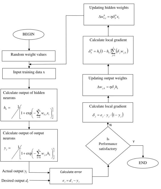
2.4 Flow chart for learning process . . . 37
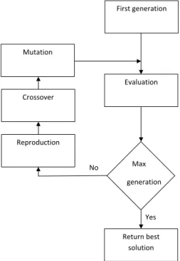
2.5 Flow chart for GA . . . 40
2.6 Five Populations . . . 47
2.7 Twenty vector differences . . . 47
2.8 Probability density function . . . 47
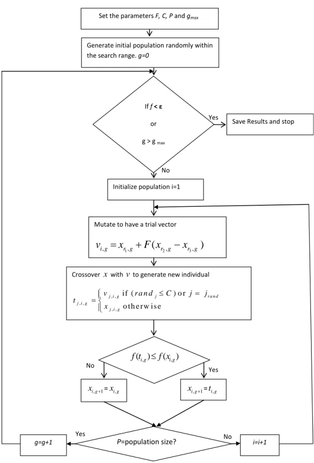
2.9 Block diagram for DE algorithm . . . 51
2.10 EC+NN identification scheme . . . 57
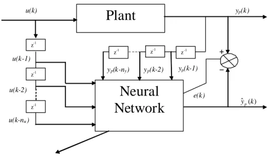
3.1 The general scheme for NARX model system identification . . . 63
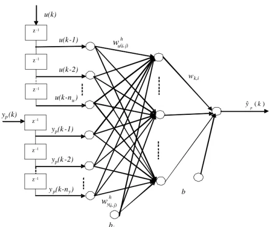
3.2 Structure of NN for NARX model system identification . . . 64
3.3 Flow chart for LM algorithm . . . 66
3.4 Identified and actual models (NN identifier) (Ex-1) . . . 75
3.5 Error in modeling (NN identifier)(Ex-1) . . . 75
3.6 Identified and actual models (DE+NN identifier)(Ex-1) . . . 76
3.7 Error in modeling (DE+NN identifier)(Ex-1) . . . 76
3.8 Identified and actual models (DE+LM+NN identifier)(Ex-1) . . 77
3.9 Error in modeling (DE+LM+NN identifier)(Ex-1) . . . 77
3.10 Identified and actual models (NN identifier)(Ex-2) . . . 79
3.13 Error in modeling (DE+NN identifier)(Ex-2) . . . 80
3.14 Identified and actual models (DE+LM+NN identifier)(Ex-2) . . 81
3.15 Error in modeling (DE+LM+NN identifier)(Ex-2) . . . 81
3.16 Identified and actual models (NN identifier)(Ex-3) . . . 82
3.17 Identified and actual models (DE+NN identifier)(Ex-3) . . . 83
3.18 Identified and actual models (DE+LM+NN identifier)(Ex-3) . . 84
3.19 Comparison of Error in modeling [NN vs. (DE + LM + NN identifier)](Ex-3) . . . 84
3.20 Hammerstein-Wiener structure . . . 85
3.21 Identified and actual models (Hammer Stein-Wiener identifier) Ex-1 . . . 86
3.22 Identified and actual models (Hammer Stein-Wiener identifier) Ex-2 . . . 86
3.23 Identified and actual models (Hammer Stein-Wiener identifier) Ex-3 . . . 87
4.1 Scheme of the memetic algorithm . . . 91
4.2 Template for proposed Memetic algorithm . . . 93
4.3 Memetic identification scheme . . . 94
4.4 BP identification performance . . . 98
4.5 Error in modeling (BP identification) . . . 98
4.6 GA identification performance . . . 99
4.7 Error in modeling (GA identification) . . . 99
4.8 GABP identification performance . . . 100
4.9 Error in modeling (GABP identification) . . . 100
4.10 PSO identification performance . . . 101
4.11 Error in modeling (PSO identification) . . . 101
4.12 PSOBP identification performance . . . 102
4.13 Error in modeling (PSOBP identification) . . . 102
4.15 Error in modeling (DE identification) . . . 103
4.16 DEBP identification performance . . . 104
4.17 Error in modeling (DEBP identification) . . . 104
4.18 A comparisons on the convergence on the MSE for all the seven methods . . . 105
5.1 The laboratory set-up: TRMS system . . . 111
5.2 Gravitational and centrifugal forces acting of the helicopter in the vertical plane . . . 113
5.3 Gyroscopic torque due to rate of change of azimuth in vertical plane . . . 114
5.4 Net torques acting on the helicopter in the vertical plane . . . . 115
5.5 Mechanical torques produced in horizontal plane . . . 116
5.6 The structure of the NN based model in terms of 1DOF horizontal119 5.7 Applied input signal to TRMS . . . 120
5.8 NLHW identification performance (pitch angle) . . . 122
5.9 NLHW identification performance (yaw angle) . . . 122
5.10 DE+LM+NN dentification performance (pitch angle) . . . 123
5.11 DE+LM+NN zoomed identification performance (pitch angle) . 123 5.12 Identification error (pitch angle) . . . 124
5.13 DE+LM+NN identification performance (yaw angle) . . . 124
5.14 DE+LM+NN zoomed dentification performance (yaw angle) . . 125
5.15 Identification error (yaw angle) . . . 125
5.16 Power spectal density for pitch . . . 126
5.17 Power spectal density for yaw . . . 126
5.18 DE and DEBP identification performance . . . 127
5.19 DE and DEBP zoomed identification performance . . . 127
5.20 Error in modeling (DEBP identification) . . . 128
5.21 Error in modeling (DE identification) . . . 128
5.22 A comparisons on the convergence on the SSE (DE, DEBP) . . 129
5.25 A comparisons on the convergence on the SSE (GA, GABP) . . 131
5.26 Error in modeling (GA identification) . . . 131
5.27 Error in modeling (GABP identification) . . . 131
5.28 PSO and PSOBP identification performance . . . 132
5.29 PSO and PSOBP zoomed identification performance . . . 132
5.30 A comparisons on the convergence on the SSE (PSO, PSOBP) . 133 5.31 Error in modeling (PSOBP identification) . . . 133
5.32 Error in modeling (PSO identification) . . . 133
6.1 Illustration of a point and its corresponding opposite in one and two dimensional spaces . . . 139
6.2 DE-NN Identification performance(Ex-1) . . . 147
6.3 ODE-NN Identification performance(Ex-1) . . . 147
6.4 DE-NN Identification error(Ex-1) . . . 148
6.5 ODE-NN Identification error(Ex-1) . . . 148
6.6 MSE(Ex-1) . . . 149
6.7 Identification performance(y(t−1), u(t−3)) (Ex-2) . . . 150
6.8 Zoomed identification performance (y(t−1), u(t−3)) (Ex-2) . . 151
6.9 MSE (y(t−1), u(t−3)) (Ex-2) . . . 151
6.10 MSE (y(t−4), u(t−5)) (Ex-2) . . . 152
6.11 Identification performance (y(t−4), u(t−5)) (Ex-2) . . . 152
6.12 Zoomed identification performance (y(t−4), u(t−5)) (Ex-2) . . 153
6.13 MSE (y(t−4), u(t−4)) (Ex-2) . . . 153
6.14 Identification Performance (y(t−4), u(t−4)) (Ex-2) . . . 154
6.15 Identification Performance(TRMS) . . . 157
6.16 Cross-correlation of input and residuals . . . 157
6.17 Auto-correlation of residuals . . . 158
6.18 Cross-correlation of input square and residuals square . . . 158
6.19 Cross-correlation of residuals and input and residuals . . . 159
7.2 RMSE for DE/best/1/exp and OMDE/best/1/exp . . . 180
7.3 RMSE for DE/rand/1/exp and OMDE/rand/1/exp . . . 180
7.4 RMSE for DE/rand-to-best/1/exp and OMDE /rand-to-best/1/exp181 7.5 RMSE for DE/best/2/exp and OMDE/best/2/exp . . . 181
7.6 RMSE for DE/rand/2/exp and OMDE/rand/2/exp . . . 182
7.7 RMSE for DE/best/1/bin and OMDE/best/1/bin . . . 182
7.8 RMSE for DE/rand/1/bin and OMDE/rand/1/bin . . . 183
7.9 RMSE for DE/rand-to-best/1/bin and OMDE /rand-to-best/1/bin183 7.10 RMSE for DE/best/2/bin and OMDE/best/2/bin . . . 184
7.11 RMSE for DE/rand/2/bin and OMDE/rand/2/bin . . . 184
7.12 Estimation of stator resistance . . . 185
7.13 Estimation of rotor resistance . . . 185
7.14 Estimation of magnetizing inductance . . . 186
2.1 Commonly used activation functions . . . 34
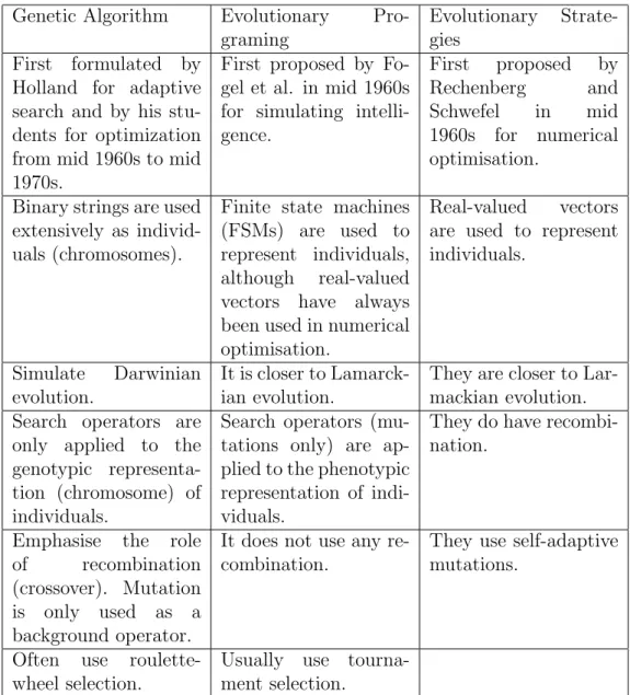
2.2 Similarities and dissimilarities between GA and other evolution-ary algorithms . . . 41
3.1 Parameters for DE+LM+NN . . . 74
3.2 Performance of the proposed methods . . . 87
4.1 Parameters used in simulation studies . . . 106
4.2 Comparison of performance of seven methods. . . 106
5.1 Parameter values for modeling TRMS . . . 118
5.2 Parameters for DE+LM+NN . . . 121
5.3 SSE for different methods . . . 134
6.1 Parameters for DE and ODE . . . 146
6.2 Comparison of training and testing errors . . . 155
7.1 Specification of the induction motor . . . 179
7.2 Parameters of the proposed DE and OMDE . . . 179
Acronyms
• BFO: Bacteria Foraging Optimization• BP: Back-propagation
• BSNN: B-spline Neural Network
• DE: Differential Evolution
• DEBP: Differential Evolution Back-propagation
• DNN: Dynamic Neural Network
• DOF: Degrees of Freedom
• EA: Evolutionary Algorithm
• EANN: Evolutionary Neural Networks
• EC: Evolutionary Computation
• ES: Evolutionary Strategy
• FNN: Feeed Forward Neural Network
• GA: Genetic Algortihm
• GABP: Genetic Algorithm Back-propagation
• GD: Gradient Descent
• IM: Induction Motor
• LM: Levenberg Marquardt
• LMS: Least Mean Square
• LSR: Least Square Regression
• MLP: Multi Layer Perceptron
• MSE: Mean Squared Error
• NARX: Nonlinear Autoregressive Exogenous
• NARMAX: Nonlinear Autoregressive Moving Average Exogenous
• NN: Neural Network
• OBL: Opposition based Learning
• ODE: Opposition based Differential Evolution
• OMDE: Opposition based Mutation Differential Evolution
• PSO: Particle Swarm Optimization
• PSOBP: Particle Swarm Optimization Back-propagation
• RBFNN: Radial Basis Function Neural Network
• RFNN: Recurrent Fuzzy Neural Network
• RLS: Recurssive Leat Square
• RMSE: Root Mean Squared Error
• SGA: Simple Genetic Algorithm
• SH: Sequential Hybridization
• SI: System Identification
• SISO: Single Input Single Output
• SSE: Sum Squared Error
• TRMS: Twin Rotor Multivariable System
Introduction
1.1
Introduction
System identification (SI) is an important research area primarily devoted to developing models of physical systems based on observed input output data. During the past three decades a lot of research has been directed towards de-veloping efficient system identification algorithms with a view to obtain models that closely match to the real physical systems. Motivated by the nice prop-erty of function approximation of Neural Networks (NNs) many research work use these networks for identification of nonlinear dynamic systems. However, selection of appropriate neural network topology, fast and efficient training are of important concerns for achieving successful system identification. Train-ing in NNs is usually guided by the minimization of an error function, such as the mean square error (MSE) or sum squared error (SSE) or root mean square error (RMSE) between actual output and estimated output averaged over all samples, by iteratively adjusting connection weights. Most training algorithms, such as back-propagation (BP) and conjugate gradient algorithms are based on gradient descent principles that often get trapped in a local mini-mum of the error function. Hence, these algorithms have the inability of finding a global minimum if the error function is multimodal and/or non-differentiable.
Recently, there is an increasing interest in exploiting evolutionary neural net-works for different applications where evolution can be introduced into NNs at
1.2 Background
different levels such as in inter layer connection weights training and architec-ture design etc. Evolutionary approaches are considered as global approaches to connection weight training of NNs, especially when gradient information of the error function is difficult to obtain. Gradient-based training algorithms often have to be run multiple times in order to avoid the problem of being trapped in a poor local optimum. Motivated by the global optimizing feature of the Evolutionary Computation (EC), recently, a lot of research works con-sider the use of evolutionary computing techniques such as Genetic Algorithm (GA), Evolutionary Algorithm (EA), Particle Swarm Optimization (PSO) and Differential Evolution (DE) etc. for efficient training of NNs. Identification problem can be conceived as an optimization problem in which the error be-tween the actual physical measured response of a system and the identified response of a model is minimized. Therefore, interest in system identifica-tion lies in minimizing the error norm of the outputs. This thesis considers the identification of nonlinear systems using a number of neuro-evolutionary approaches. It has been demonstrated in this work that the success of the combined use of local and global search methods for training of the neural network yields efficient nonlinear system identification strategy.
1.2
Background
1.2.1
System Identification
The first step in designing the controller is to model the plant. System identifi-cation is the process of building models of dynamic process from input-output signals. The aim of system identification [1] can be identified as to find a model with adjustable parameters and then to adjust them so that the pre-dicted output matches the measured output. Two important points on system identification are:
• Which model parameterization is to be used?
Most of system identification techniques have their roots in statistical meth-ods like Least squares fitting, maximum likelihood estimation etc. Apart from parametric methods of system identification there are non-parametric tech-niques for system identification such as spectral analysis, correlation analysis and transient analysis. The various steps involved in system identification are experiment setup and data collection, data preprocessing, model structure selection, parametric estimation and validation. In nonlinear system identi-fication [2] one approach is the black box model that uses various selected model structures and the model that gives optimum fit for the test data is the identified model.
Linear system identification
A linear system obeys two properties namely superposition and scaling. Hence, if f is a linear operator given by
y1(t) =f(u1(t)) (1.1)
y2(t) =f(u2(t)) (1.2)
where, u1, u2, y1 and y2 are the inputs and outputs of the system, then
ac-cording to the definition of linearity, we have
f(k1u1(t) +k2u2(t)) =k1y1(t) +k2y2(t) (1.3)
where k1 and k2 are constants.
Parametric representations
A parametric model consists of a set of differential or difference equations which describe the system dynamics. Such equations usually contain a small number of parameters, which can be varied to alter the behavior of the equations. The identification of an unknown system comprises two stages. First, the structure of the parametric model is chosen, and then the parameters themselves are
1.2 Background
estimated by using an optimization algorithm.
Linear Difference Equations
We can write the relationship between the input, output, and noise as a linear difference equation given by
y(t) +a1y(t−1) +...+anxy(t−nx) =b1u(t−1) +b2u(t−2) +...bnyu(t−ny)+
e(t) +c1e(t−1) +...+cnze(t−nz)
(1.4) which can be written more compactly as
A(q)y(t) =B(q)u(t) +C(q)e(t) (1.5) where A(q) = 1 +a1q−1+...+anxq −nx B(q) = b1+b2q−1+...+bnyq −ny+1 C(q) = 1 +c1q−1+...+cnzq −nz
q−1 is the backward shift operator. This is the auto-regressive, moving
av-erage exogenous (ARMAX) model. The current output y(t) depends on an exogenous input u(t), an innovations process e(t) and the past values of the output. The polynomials (A(q), B(q) ) known as deterministic model, whereas ( A(q), C(q) ) represent the stochastic system model. This model has several special cases, the first of which is the autoregressive (AR) model:
A(q)y(t) = e(t) (1.6)
in which the output depends on the current disturbance, as well as the previous values of the output. Another special case is the moving average (MA) model:
in which the output depends on the previous values of the disturbance, Com-bining these two, we get the autoregressive moving average (ARMA) model:
A(q)y(t) =C(q)e(t) (1.8) If we add an accessible input, u(t), to the AR model, the result is an auto-regressive exogenous input (ARX) model:
A(q)y(t) =B(q)u(t) +e(t) (1.9) A special case of the ARX structure, in which there is no disturbance input, is the finite impulse response (FIR) model:
y(t) =B(q)u(t) (1.10)
In this case, the output depends solely on the previous values of the exogenous input. This structure forms the basis of a number of so-called non-parametric identification schemes. Once a candidate model structure and order have been chosen, the model representation can be reduced to a parameter vector, θ = [A(q)B(q)C(q)]
State Space Models
Another parametric system representation is the state space model. In this case, we consider a set of equations of the form:
x(t+ 1) =Ax(t) +Bu(t) (1.11)
y(t+ 1) =Cx(t) +Du(t) (1.12) where the sequences u(t), y(t) and x(t) represent the system’s input, output and state respectively. The impulse response (Markov parameters) of the sys-tem is first identified from input-output data, and then used to compute the system matrices A,B,C and D.
1.2 Background
Nonparametric representations
A linear system can be represented by its impulse response. In continuous time, we can compute the output via the convolution integral: [20]
y(t) =
T Z
0
h(τ)u(t−τ)dτ (1.13)
whereT is the memory length of the system, andh(τ) is the impulse response. In this case, as the lower bound of the integration is 0, the system is causal. Given that the analysis will be performed using sampled data on a digital computer, we will require a discrete time formulation. One benefit gained by restricting ourselves to discrete time is that it avoids the mathematical difficul-ties associated with a continuous-time white-noise signal. In continuous time, a white noise signal has infinite bandwidth and hence infinite power. In discrete time, however, it is simply a sequence of independently distributed random variables. In discrete time, the convolution integral becomes the summation:
y(t) = ∆t.
T−1
X τ=0
h(τ)u(t−τ) (1.14)
Here, the memory length, T, and the lag τ, are integers. If the system is non causal, then the lower limit of the summation will be negative. The sampling increment is ∆t; which is assumed to be 1 here so that it can be dropped. If the input process is white, it can be shown that the impulse response can be recovered from the input/output cross-correlation function. Given N data points, a biased estimate of the cross-correlation can be obtained as:
ˆ Φuy(τ) = 1 N N X t=τ+1 u(t−τ)y(t) (1.15)
Substituting the value y(t) of from (1.14) in (1.15) we have ˆ Φuy(τ) = N1 N P t=τ+1 u(t−τ) T−1 P j=0 h(j)u(t−j) = T−1 P j=0 h(j) 1 N N P t−τ+1 u(t−τ)u(t−j) = T−1 P j=0 h(j) ˆΦxx(τ−j) (1.16)
Hence, from equation (1.16) the input-output cross-correlation is equal to the convolution of the impulse response with the input auto-correlation function. If the input is white, the auto-correlation function is an impulse, and the cross-correlation and impulse response are equal. If the input is non-white, the input auto-correlation function must be deconvolved, from the cross-correlation es-timate. This problem was approached by modeling the observed input as a white noise process filtered by an autoregressive filter. This filter can be esti-mated, and its inverse (a moving average filter) applied to both the input and output signals. The cross-correlation between the filtered input and filtered output is then estimated. Since the filtered input signal is effectively white, the cross-correlation estimate provides an estimate of the impulse response [20]. The input auto-correlation is estimated, and the convolution between the input auto-correlation and the impulse response can be written in matrix form as: ˆ φuy(0) ˆ φuy(1) .. . ˆ φuy(T −1) = ˆ φuu(0) φˆuu(1) · · · φˆuu(T −1) ˆ φuu(1) φˆuu(0) · · · φˆuu(T −2) .. . ... ... ˆ φuu(T −1) φˆuu(T −2) · · · φˆuu(0) h(0) h(1) .. . h(T −1) (1.17) This equation can be solved efficiently, using Levinson’s algorithm [3], since
ˆ
φuu, is the matrix derived from the input auto-correlation function, has a
1.2 Background
Nonlinear system identification
Nonlinear system identification is the task of determining or estimating a sys-tems input-output relationship F, based on (possibly noisy) output measure-ments.
y(t) =F [x(t)] +e(t) (1.18)
where e(t) is the noise, disturbance or another source of error in the pro-cess of measurement. Nonlinear systems can be modeled into nonparametric and parametric forms. In parametric modeling the input-output relationship are defined by finite number of parameters. Nonparametric nonlinear system identification includes the Volterra and Wiener series models which are based on Taylor series expansion of time invariant nonlinear systems. The Volterra model expresses the input-output relationship of a nonlinear system in terms of Volterra kernels. The output y(t) in response to the input x(t) can be expressed as y(t) =h0+ ∞ X n=1 ∞ Z −∞ · · · ∞ Z −∞ hn(τ1,· · ·, τn)x(t−τ1)· · · x(t−τn)dτ1· · · dτn (1.19) whereh0is a constant andhj(τ1· · · ·τj), 1≤j ≤ ∞is thejthorder Volterra
kernel coefficients defined for τi = −∞ to +∞, i = 1, 2,· · ·, n. We assume
hj(τ1,· · ·, τj) = 0 if any τi < 0, 1 ≤ i ≤ j which implies causality. In
para-metric nonlinear system models, the input-output relation can be expressed by a mathematical function determined by a finite number of parameters. Parametric models can be viewed as special case of nonparametric models. Truncated N-th order Volterra series can be taken as parametric nonlinear system model described as
y(t) = h0+ N X n=1 ∞ Z −∞ · · · ∞ Z −∞ hn(τ1· · · ·τn)x(t−τ1)· · · x(t−τn) dτ1· · · dτn (1.20)
Linear-in-parameter models
Parametric representations of nonlinear systems typically contain a small num-ber of coefficients that can be varied to alter the behavior of the equation and may be linked to the underlying system. Leontaritis and Billings [4] have proposed the NARMAX structure as a general parametric form for modeling nonlinear systems. This structure is suitable for modeling both the stochastic and deterministic components of a system and capable of describing a wide variety of nonlinear systems [5, 6, 7, 8]. NARMAX models have been success-fully demonstrated for modeling the input output behavior of many complex systems such as adaptive polynomial filters, and offer a promising framework for describing nonlinear behavior such as aircraft dynamics. Often, this for-mulation yields compact model descriptions that may be readily identified and afford greater interpretability. This system representation, however, can yield a large number of possible terms required to represent the dynamic process. In practice, many of these candidate terms are insignificant and can be removed. Consequently, the structure-detection problem turns out to be selection of a subset of candidate terms that best predicts the output while maintaining an efficient system description.
NARMAX models also describe nonlinear systems in terms of linear in the pa-rameters difference equations, which represent the current output with present and past inputs and, past outputs. Identifying a NARMAX model requires two distinct steps such as structure detection and parameter estimation. Structure detection can be divided into steps such as model order selection and selection of parameters to include in the model. We consider model order selection as part of structure detection since, theoretically, there are an infinite number of candidate terms that could be considered initially. Establishing the model order limits the choice of terms to be considered. Good parameter estimation methods can be explored if the model order is known. However, there remains a problem in model order selection. Depending on the order of the system, the
1.2 Background
number of candidate terms can be very large. Selection of a subset of these candidate terms is necessary for an efficient system description. In fact, many NARMAX systems can be described by only a few terms. A wide range of dis-crete time multiple variable nonlinear stochastic systems can be represented by the following NARMAX model:
ˆ
y(t) =α+Fl[y(t−1), ..., y(t−nx), u(t), ..., u(t−ny), e(t−nz)] +e(k)
(1.21)
where y(t), u(t) and e(t) represent the system output, input, and prediction error, respectively. Also, l is the degree of nonlinearity, α is a constant dc level, Fl[.] is some vector valued nonlinear function, n
x, ny and nz represent
the number of lags in the input, output and prediction error, respectively. The prediction error term e(t), defined as e(t) = y(t)−yˆ(t), is included in the model to accommodate noise, where ˆy(t) is the prediction output. Expanding Eq. (1.21) by defining the function Fl[.] as a polynomial of degree l gives
a representation of all the possible combinations of y(t), u(t) and e(t) up to degree l. For example, the current output can be presented as
y(t) = α+θ1y(t−1)+θ2u(t−1)+θ3u(t−1)y(t−1)+θ4u(t−1)e(t−1)+θ5e(t−1)+e(t)
By defining
p1(t) =y(t−1), p2(t) =u(t−1), p3(t) =u(t−1)y(t−1),
p4(t) =u(t−1)e(t−1), p5(t) =e(t−1), p0(t) = 1, andθ0 =α
IfN input and output measurements are available, and if there areM terms in the model, then the above equation can be written in a matrix form as
Y =Aθ+e (1.22)
where
YT = [y(1) y(2) · · · y(N)]
eT= [e(1) e(2) · · · e(N)] A= A0(1) A1(1) · · · AM(1) A0(2) A1(2) · · · AM(2) .. . ... ... A0(N) A1(N) · · · AM(N)
where A represents a term in the NARMAX model and θ represents the unknown parameters to be estimated. The parameter vector θT in Eq. (1.22)
can be estimated using some well known methods, such as a least-squares-based or prediction error method, Choleski or U−D factorization, the Q−R
algorithm, singular value decomposition or principle component regression. Nonlinear-in-parameter models
This class of models include all parametric descriptions of nonlinear systems whose output is not linearly related to the parameters. Nonlinear-in-parameters models often arise from physical modeling considerations. In general, it can be expressed as y(t) = F [x(t), θ] where F has a fixed functional form that is parameterized by θ. Neural networks are the most well-known class of nonlinear-in-parameter models [16]. The hidden nodes represent the nonlinear processing units and the link between the nodes represent the weighting factor to the input of each neuron. These weights are the parameters of the neural network model. As the neurons are the nonlinear functions, the output of the network is the nonlinear functions of the parameters. Multi layer perceptrons are nonlinear-in-parameter models so the identification method must include a nonlinear optimization technique such as nonlinear least square, prediction estimation error method etc. It will be discussed later that there remains se-rious problem of local minima in using these optimization techniques.
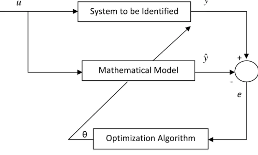
The basic block-diagram representation of an identification problem is shown in Fig. 1.1. From the figure it is clear that if the error tends towards zero the estimated output will be same as the desired output. So the identified model
1.2 Background
will exactly mimic the original system to be identified.
System to be Identified Optimization Algorithm e + ‐ θ u y ˆ y Mathematical Model
Figure 1.1: Block Diagram on System Identification
As shown in Fig.1.1, given the discrete time, time invariant nonlinear dy-namic system of inputs u(k) and outputs y(k). The objective is to develop identification algorithms using several methods such as evolutionary comput-ing techniques and neural networks. The NARX model structure is taken as the nonlinear frame work which is in the form of
yk =f(y(k−1),· · ·, y(k−ny);u(k);u(k−1),· · ·, u(k−nu)) (1.23)
<k = [y(k−1),· · ·, y(k−ny);u(k);u(k−1),· · ·, u(k−nu)] where k ∈ Z+is
the discrete temporal variable
uk ∈R1 is the input at time k
yk∈R1 is the output at time k
f :Rny+nu is an unknown nonlinear mapping defined on an open set
ny is an integer denote maximum lag in the output
nu is an integer denote maximum lag in the input
<k is the regression vector in a NARX model
Sincef is unknown, the objective is to use some type of network approximator Γ (<, θ) to approximate f(<). In the network, < ∈Rn is the input to the net-work and θ∈Rd is set of adjustable parameter in vector form ofd dimension.
The system described in equation (1.23) can be rewritten in the form as
yk = Γ (<(k);θ∗) +e(k) (1.24)
where ise the modeling error, defined as
e(k) =f(<(k))−Γ (<(k);θ∗) (1.25) In order to obtain successful identification the identified system must be able to reproduce the output of the physical system for any given input. Let <k
belongs to some compact set Z for all k > 0, then we define the parameter vector θ∗ as the optimal value of θ in the sense that it minimizes the distance between fand Γ for all < ∈Z. The optimal parameter vectorθ∗ is defined as
θ∗ = arg min sup <∈Z |f(<)−Γ(<;θ)| (1.26) The optimization problem requires finding a vector θ ∈ S, where S is the search space, so that a certain quality criterion is satisfied, namely that the error norm is minimized. By changing the value of θ it is possible to change the input-output response of the network Γ. The search space S is defined by a set of maximum and minimum values for each parameter. The vector θis an
d dimensional domain where each element θi is bounded with θmax and θmin
containing the upper bounds and lower bounds of the d parameters respec-tively i.e.
S=θ ∈Rd|θmin,i ≤θi ≤θmax,i ∀i= 1,2,· · · , d .
1.2.2
Neural Networks
A neural network [9, 10] consists of a set of processing elements, also known as neurons or nodes, which are interconnected. It can be described as a directed graph in which each nodei performs a transfer function fof the form
yi =f n X j=1 wi,jxj−bi ! (1.27)
1.2 Background
where yi is the output of the node i, xj is the jth input to the node i, and
wi,j is the connection weight between nodes i and j, bi is the threshold (or
bias) of the node. Usually, f is nonlinear, such as a heaviside, sigmoid, or Gaussian function. NNs can be divided into feed-forward and recurrent classes according to their connectivity. A NN is feed-forward if there exists a method which numbers all the nodes in the network such that there is no connection from a node with a large number to a node with a smaller number. All the connections are from nodes with small numbers to nodes with larger num-bers. A NN is recurrent if such a numbering method does not exist. In (1.27), each term in the summation only involves one input. The architecture of a NN is determined by its topological structure, i.e., the overall connectivity and transfer function of each node in the network. Learning NN is otherwise known as training of NN because the learning is achieved by adjusting the con-nection weights iteratively so that trained NN can perform certain tasks. This Learning is roughly divided into supervised, unsupervised, and reinforcement learning. Supervised learning is based on direct comparison between the esti-mated output of a NN and the desired correct output, also known as the target output. It is often formulated as the minimization of an error function such as the total mean square error between the actual output and the estimated output summed over all available data. A gradient descent based optimization algorithm such as backpropagation [64] can then be used to adjust connection weights in the NN iteratively in order to minimize the error. Reinforcement learning is a special case of supervised learning where the exact desired output is unknown. It is based only on the information of whether or not the actual output is correct. Unsupervised learning is solely based on the correlations among input data. No information on correct output is available for learning. The essence of a learning algorithm is the learning rule, i.e., a weight-updating rule which determines how connection weights are changed. Examples of pop-ular learning rules include the delta rule and backpropagation. These will be discussed in chapter 2.
1.2.3
Evolutionary Algorithms
Evolutionary algorithms are based on computational models of fundamental evolutionary processes such as selection, recombination and mutation. Fig. 1.2 gives an overview of a general evolutionary algorithm. Individuals, or cur-rent approximations are encoded as strings composed over some alphabet(s), e.g. binary, integer, real valued etc., and an initial population is produced by randomly sampling these strings. Once a population has been produced it may be evaluated using an objective function which characterizes an individual performance in the problem domain. The objective function is also used as the basis for selection and determines how well an individual performs in its environment. A fitness value is then derived from the raw performance mea-sure given by the objective function and is used to bias the selection process. Highly fit individuals will have a higher probability of being selected for re-production than individuals with a lower fitness value. Therefore, the average performance of individuals can be expected to increase as the fitter individuals are more likely to be selected for reproduction and the lower fitness individu-als get discarded. Selected individuindividu-als are then reproduced, usually in pairs, through the application of genetic operators. These operators are applied to pairs of individuals with a given probability and result in new offspring that contain material exchanged from their parents. The offspring from reproduc-tion are then further perturbed by mutareproduc-tion. These new individuals then make up the next generation. These processes of selection, reproduction and eval-uation are then repeated until some termination criteria are satisfied, e.g. a certain number of generations completed, a mean deviation in the performance of individuals in the population or when a particular point in the search space is reached.
1.2 Background
procedure EA {
t = 0
;
initialize
P(t)
;
evaluate
P(t);
while not finished do {
t = t + 1
;
select
P(t)
from
P(t-1);
reproduce pairs in
P(t)
;
mutate
P(t);
evaluate
P(t);
}
}
Figure 1.2: A Simple Evolutionary Algorithm
In general, most real world optimization problems have several challenging properties. Almost of all problems have a significant number of local optima, and the search space can be so huge that the exact global optimum cannot be found in reasonable time. Further, the problems may have multiple conflicting objectives that should be considered simultaneously (e.g., cost versus quality). Moreover, there may be a number of nonlinear constraints to be fulfilled by the final solution. Furthermore, the problem may have dynamic components al-tering the location of the optimum during the optimization process. For some problems, variants of the local search approach have proven to be very efficient, e.g., Lin-Kernighan algorithm for the Traveling Salesman Problem. However, deterministic local search algorithms, such as steepest decent, do not allow a decrease in the solutions quality during the search. For this reason, these algorithms often stagnate at a local optimum, which makes local search less desirable for many real-world problems. Valuable alternatives are stochastic search methods such as simulated annealing, Tabu search, and evolutionary
algorithms. Among these techniques, EAs seem to be a particularly promis-ing approach for several reasons. EAs are very general regardpromis-ing the problem types they can be applied to continuous, mixed-integer and combinatoric type problems. Furthermore, these algorithms can easily be combined with existing techniques such as local search methods. In addition, it is often straightfor-ward to incorporate domain knowledge in the evolutionary operators and in the seeding of the population. Moreover, EAs can handle problems with any combination of the above mentioned challenges in real-world problems i.e. lo-cal optima, multiple objectives, constraints, and dynamic components. In this connection, the main advantage lies in the EAs population-based approach. For local optima, the genetic diversity of the population allows the algorithm to explore several areas of the search space simultaneously. There is of course no guarantee on the premature convergence to a local optimum, but the pop-ulation improves the EAs robustness on such problems. Naturally, EAs do also have some disadvantages. Unfortunately, they are rather computation-ally demanding, since many candidate solutions have to be evaluated in the optimization process. However, recently there has been an increase interest in dealing with this problem and some techniques have been suggested such a hybrid EAs to make it faster.
1.3
Literature Survey on System Identification
The theory of system identification for linear systems is matured during the last two decades and there exist useful tools based on Least Mean Square (LMS), Recursive Least Square (RLS), Kalman Filtering [1] etc. Many problems in control engineering, signal processing and machine learning can be cast as a system identification problem where the task is to determine a suitable model from a given set of input-output data. The resulting model can then be used for the prediction and control of a ”black- box” system. In reality, however, all sys-tems are more or less nonlinear. In recent years there has been a lot of research pursued on nonlinear system identification. A survey of existing techniques of
1.3 Literature Survey on System Identification
nonlinear system identification prior to 1980s is given by Billings [2], a survey of the structure detection of input-output nonlinear systems can be obtained in [5], and a survey of nonlinear black-box modeling in system identification can be found in [7]. Several methods have been developed for the identification and control of nonlinear system, including NARMAX, Hammerstein, Wiener or Hammerstein-Wiener structures, but these methods suffer the difficulty of representing the behavior of the system over its full range of operation [6]. For nonlinear system identification, NARX model has been implemented by the authors [4, 8]. The extra complexity associated with nonlinear system identification, particularly when there is no initial information or model struc-ture detail. One successful approach to this problem is the orthogonal Least Squares Regression (LSR) method to find a suitable set of nonlinear terms for the system.
Since eighties, neural networks have been extensively applied to the identi-fication of nonlinear dynamical systems. Most of the works are based on mul-tilayer feed-forward neural networks with back-propagation learning algorithm [68, 70]. In neural network based identification, the selection of the number of hidden nodes and the number of hidden layers (i.e. the structure of the net-work) corresponds to the model selection stage. The network can be trained in a supervised manner with a back-propagation algorithm, which is based on an error-correction learning rule. The error signal is propagated backward through the network. The back-propagation algorithm utilizes gradient de-scent to determine the weights of the network and hence corresponds to the parameter estimation stage. Both feed-forward and recurrent networks can be used for identification purposes. The feed-forward network provides a nonlin-ear static map between inputs and outputs of the neural network. A number of theoretical and practical system identification problems have been solved us-ing neural network approach with multi-layered perceptron (MLP) with back-propagation training [16, 17]. In [18] the author has used a radial basis function
neural network (RBFNN) for the nonlinear system identification problem. The Wavelet networks techniques [19] were also applied to system identification of nonlinear systems in which adaptive techniques such as back propagation al-gorithm found to provide better accuracy compared to non-adaptive ones such as Volterra series, Wiener-Hammerstein modeling and polynomial methods. A novel multilayer discrete-time neural network is presented in [21] for identifi-cation of nonlinear dynamical systems. In [22], a scheme for on-line states and parameters estimation of a large class of nonlinear systems using RBFNN has been designed. An approach to control nonlinear discrete dynamic systems, which relies on the identification of a discrete model of the system by a feed-forward neural network with one hidden layer, is presented in [23]. Nonlinear system identification using discrete-time recurrent single layer and multilayer NNs are studied in [24]. An identification method for nonlinear models in the form of Fuzzy-Neural Networks is introduced in [25]. This Fuzzy-Neural Net-works combine fuzzy if-then rules with NNs. An adaptive time delay NN is used for identification of nonlinear systems in [26]. Onder and Kaynak in [27] investigated the identification of nonlinear systems by feed-forward NNs, ra-dial basis function NNs and adaptive neuro-fuzzy inference systems. Authors in [28] have discussed about a least squares support vector machine (SVM) re-gressor used for generating the control actions, while an SVM-based tree-type neural network is used as the critic.
However, the complexity and the combinatorial growth in the search space mean that exhaustive search is not always feasible and is limited in applica-tion. Conventional training algorithms mainly rely on gradient based tech-niques. Although these techniques suffice in many applications, they require a differentiable performance index or a smooth search space. This condition may not always be satisfied in practical applications because of noisy data or system discontinuity. Even when the derivative or gradient information is available these techniques often result in a local optimum if the solution space
1.3 Literature Survey on System Identification
is multi-modal. They may also fail completely, if the space is noisy as found in practical applications. These problems can become more complex if the plant to be identified is multiple-input and multiple-output system. Further, the following difficulties exist with conventional techniques.
• Initial information of the parameters usually need to be known a priori.
• The estimation may be biased if the measurement or process noise is correlated.
• It is difficult to identify the transport delays.
• Input-Output data at steady state may cause problems in matrix manip-ulations, as they have very close value.
• It is difficult to estimate parameters that are not linearly separable. Compared to the conventional approaches which search the term space iter-atively, building a more and more complex model, the EA based approach conducts a global and robust search of the model space. Thus, the EA has the potential to be more effective in identifying a suitable model structure and hence more general in nature. Contribution to the system identification using EAs is discussed in [29, 30, 31, 32, 33, 34, 35]. In [29] the authors proposed a genetic algorithm based on NARX system identification algorithm. In [30] an inversion control of nonlinear system with an inverse NARX model iden-tification using genetic algorithms has been proposed. Authors in [31] have implemented nonlinear system identification using a subset selection method and LSR using GAs. In [32] the authors have discussed about the identification of structural system using an evolutionary strategy. Models for evolutionary algorithm and their application in system identification are addressed in [33]. Authors in [35] have implemented the genetic algorithms to estimate the Pa-rameter of a robot arm. The GA is used to select a fixed number of terms from a set of possible nonlinear terms and LSR is used to identify the param-eters of those terms. Because the EA operates on a population of solution
estimates, the EA produces a family of low-variance models which can be as-sessed according to different criteria before a final model is chosen. From the previous neural network system identification approaches, it is observed that even neural network has been proved to be a successful technique for nonlinear system identification but there still remains little concern about its conver-gence and problem of being trapped at local minima. Evolutionary neural networks (EANNs) refer to a special class of neural networks in which evolu-tion is another fundamental form of adaptaevolu-tion in addievolu-tion to learning [36, 37].
In [38], the author has applied genetic algorithms to obtain the values of the weights of both the feed-forward and feedback connections. It describes the use of genetic algorithms to train the Elman and Jordan networks for dynamic systems identification. In [39] a genetic algorithm is proposed to design wavelet neural networks (WNNs) for nonlinear system identification. By introducing a connection switch to each link between a wavelet and an input node, the decomposition is done automatically during the evolutionary process. GA is used to train the wavelet parameters and the connection switches. In this way, both the structure and wavelet parameters of WNNs are optimized simultane-ously. Evolving wavelet neural networks for system identification is discussed by the authors [40]. A new encoding scheme for training RBF networks by genetic algorithms is proposed by the authors [41]. In the proposed encoding scheme, both the architecture (numbers and selections of nodes and inputs) and the parameters (centers and widths) of the RBF networks are represented in one chromosome and evolved simultaneously by GAs so that the selection of nodes and inputs can be achieved automatically. The performance and ef-fectiveness of the presented approach are evaluated using two benchmark time series prediction examples and one practical application example, and are then compared with other existing methods. It is shown by the simulation tests that the developed evolving RBF networks are able to predict the time series accu-rately with the automatically selected nodes and inputs. In [42], both off-line
1.3 Literature Survey on System Identification
architecture optimization and on-line adaptation have been developed for a dy-namic neural network (DNN) in nonlinear system identification. A series of GA operations are applied to the connection matrices to find the optimal number of neurons on each hidden layer and interconnection between two neighboring layers of DNN. The hybrid training is adopted to evolve the architecture, and to tune the weights and input delays of DNN by combining GA with the mod-ified adaptation laws. The modmod-ified adaptation laws are subsequently used to tune the input time delays, weights and linear parameters in the optimized DNN-based model in on-line nonlinear system identification. An approach to nonlinear system identification using evolutionary Neural Networks and LMS algorithm has been proposed by the authors in [43]. A PSO tuned radial basis function network model is proposed for identification of nonlinear systems in [44]. At each stage of orthogonal forward regression (OFR) model construction process, PSO is adopted to tune one RBF unit’s centre vector and diagonal covariance matrix by minimizing the leave-one-out (LOO) MSE. In [45] the author has presented a learning algorithm for dynamic recurrent Elman neu-ral networks based on a modified particle swarm optimization. The proposed algorithm has been applied to perform speed identification and to design a controller to perform speed control for Ultrasonic Motors (USM). The contri-bution in [46] concerns with the design of a generalized functional-link neural network with internal dynamics and its applicability to system identification by means of multi-input single output nonlinear models of autoregressive with ex-ogenous inputs type. A GA based evolutionary multi-objective optimization in the Pareto-sense is used to determine the optimal architecture of that dynamic network. The contributions in [47] proposed the application of a modified arti-ficial immune network inspired optimization method - the opt-aiNet - combined with sequences generate by Henon map to provide a stochastic search to adjust the control points of a B-spline neural network (BSNN). The numerical results presented here indicate that artificial immune network optimization methods are useful for building good BSNN model for the nonlinear identification of
two case studies: (i) the benchmark of Box and Jenkins gas furnace, and (ii) an experimental ball-and-tube system. Authors in [48] outlined the basic con-cept and principles of two simple and powerful swarm intelligence tools: the PSO and the BFO. The adaptive identification of an unknown plant has been formulated as an optimization problem and then solved using the PSO and BFO techniques. Using this approach efficient identification of complex non-linear dynamic plants have been carried out through simulation study. One such evolutionary computation i.e. DE, was first introduced in [49], is suc-cessfully applied to many artificial and real world optimization problems with applications. A differential evolution based neural network training algorithm was first introduced in [50]. Authors in [51] proposed an effective DE based learning algorithm for recurrent fuzzy neural network (RFNN) with fuzzy in-puts, fuzzy weights and biases, and fuzzy outputs. The effectiveness of the proposed method is illustrated through simulation of benchmark forecasting and identification problems and comparisons with the existing methods. The suggested approach has also been used for real applications in an oil refinery plant for petrol production forecasting.
The major disadvantage of the EANN [36, 37] approach is that it is com-putationally expensive and has slow convergence. With a view to speed up the convergence of the search process, a number of different gradient methods such as LM and BP are combined with evolutionary algorithms. These are the new class of hybrid algorithms i.e. global evolutionary search supplemented by local search techniques. It may be noted that the local search methods when used alone there may be problem for getting trapped in local minima. The hybridization of these local searches with evolutionary techniques is useful to either accelerate the discovery of good solutions, for which evolution alone would take too long to discover, or to reach solutions that would otherwise be unreachable by evolution or a local method alone. It is assumed that the evolutionary search provides for a wide exploration of the search space while
1.3 Literature Survey on System Identification
the local search can somehow zoom-in on the basin of attraction of promising solutions. The natural analogies between human evolution and learning, i.e. EAs and neural networks prompted a great deal of research into the use of hybrid algorithms such as memetic algorithms to evolve the design of NNs.
Memetic algorithms (MAs) have been proven very successful across a wide range of problem domains such as combinatorial optimization [57], optimiza-tion of non-staoptimiza-tionary funcoptimiza-tions [52], multi-objective optimizaoptimiza-tion [53], bioin-formatics [54], etc. MAs have received various names throughout the literature and scientist not always agree what is and what is not an MA due to the large variety of implementations available. Some of the alternative names used for this search framework are hybrid GAs, Baldwinian EAs, Lamarckian EAs, ge-netic local search algorithms, etc to cover a wide range of techniques where evolutionary-based search is augmented by the addition of one or more phases of local search. Research in memetic algorithms has progressed substantially, and several Ph.D. dissertations have been written analyzing this search frame-work and proposing various extensions to it [55, 56, 57, 58]. In [59], the authors have proposed an effective PSO based memetic algorithm for designing arti-ficial neural network where an effective adaptive Meta-Lamarckian learning strategy is employed to decide which local search method to be used so as to prevent the premature convergence and concentrate computing effort on promising neighbor solutions. Authors in [60] propose two hybrid evolutionary algorithms as alternatives to improve the training of dynamic recurrent neural networks.
However, a lot more research is needed to achieve the faster convergence and obtaining global minima. Hence there has been a great interest in combining training and evolution with neural networks in recent years.
1.4
Objectives of the Thesis
The objectives of the thesis are as follows
• To develop efficient nonlinear system identification algorithms using evo-lutionary computing techniques and neural networks.
• To combine evolutionary algorithm and gradient descent (GD) learning for overcoming the problems of local minima during training of the NNs with GD learning.
• To prove the convergence of the proposed neuro-evolutionary hybrid sys-tem identification algorithms.
• To achieve improved identification of nonlinear systems including multi-input multi-output (MIMO) systems introducing a memetic differential evolution algorithm and to compare its performance with other memetic algorithms.
• To devise a new variant differential evolution algorithm with improved search ability for identifying different types of nonlinear systems.
• To propose opposition based mutation differential evolution algorithm based identification algorithm with application to nonlinear system for estimating the parameters of an induction motor.
1.5
Motivation of the Present Work
Determination of efficient structure and weights of a NN become a challenge in the field of nonlinear system identification. The other challenge of applying evolutionary NN is that most evolutionary algorithms [71, 72, 75, 157, 158, 159] will not provide good optimal performance if not fine-tuned in local search al-though they are good at the global search. Hybridization can improve the efficiency of evolutionary training by incorporating a local search procedure such as BP [78], LM [69] or other random search algorithm into the evolution,
1.6 Thesis Organization
i.e., combining global search ability with local search’s ability to fine tune.
1.6
Thesis Organization
Chapter 1, gives an overview of system identification techniques and dis-cusses about the application of neural networks and evolutionary computation for system identification. It describes techniques that are suitable for building models of nonlinear systems. This chapter reviews various representations used to describe linear systems and the methods used to identify them from measure-ments of input-output data. Subsequently, it considers different descriptions of nonlinear systems and the techniques used in system identification. It also describes about the nonlinear system identification using linear-in-parameter models such as NARMAX modeling followed by nonlinear- in-parameter mod-els i.e. neural modmod-els. Subsequently it discusses the contribution of the thesis followed by organization of this thesis.
Chapter 2, starts with discussion about the NNs and their training. A gradi-ent descgradi-ent-based optimization algorithm such as back-propagation is discussed which is used to adjust connection weights in the NN iteratively in order to minimize the training errors. A weight-updating rule i.e. delta rule which determines how connection weights are changed has been discussed next. Sub-sequently, the chapter focuses on different types of evolutionary algorithms and population based search strategies i.e. how individuals in a population compete and exchange information with each other in order to perform certain tasks. The essence of this chapter is to discuss about finding a near-optimal set of connection weights for a neural network. The chapter is concluded with discussions about the need of improving training of neural networks so that optimal set of connection weights can be achieved.
neu-ral network and LM. Here, DE and LM in a combined framework are used to train a NN for achieving better convergence of neural network weight op-timization. In this chapter the LM is used as a local optimizer after the DE algorithm. This type of algorithms are known as SH where set of algorithms is applied one after another, each using the output of the previous as its input. As DE becomes slow near the basin of the global optimization the function of LM is to enhance the speed of convergence. In this chapter number of exam-ples including a practical case-study has been considered for implementation of this algorithm.
Chapter 4, describes a memetic algorithm approach for the training of ar-tificial neural networks, i.e. how memetic algorithm trained MLP applied to nonlinear system identification. The MAs are used as an alternative to gradi-ent search methods, such as BP, which have shown limitations when dealing with rugged landscapes with many poor local optima. The work described in this chapter aims at designing a training strategy that is able to cope up with difficult error manifolds, and to achieve perfectly trained neural networks that produce small training errors. A rigorous study on the identification of a nonlinear system using seven different algorithms namely BP, GA, PSO, DE, genetic algorithm back-propagation (GABP), paricle swarm optimiza-tion back-propagaoptimiza-tion (PSOBP) along with the proposed differential evoluoptimiza-tion back-propagation (DEBP) approaches has been done. In the proposed system identification scheme, three global searches have been combined with the gra-dient descent method i.e. the BP algorithm to overcome the slow convergence of the evolving neural networks. The local search BP algorithm is used as an operator like crossover and mutation operator for GA, PSO and DE. These algorithms have been tested on standard benchmark problems given in [61, 62] for nonlinear system identification to prove their efficacies.
1.6 Thesis Organization
rig, a twin rotor multi-input multi-output (TRMS) using SH and MA. The TRMS is a highly nonlinear system which can be considered as an experimen-tal model of a complex air vehicle. Such vehicles are required to be identified precisely to ensure satisfactory control performance to meet the demand for automation. This implies that linear characterization of aircraft’s is not good to describe the systems characteristics for control purposes and nonlinear mod-eling techniques are required. Neural network based nonlinear characterization are promising approaches. This chapter focuses into the development of non-linear modeling of a TRMS using SH and MA. The system is modeled using a NARX identification scheme with a feed-forward neural network. In this chapter the responses of all the identified models are compared with that of the real TRMS to validate the accuracy of the models.
Chapter 6, discusses a new variant of the DE called ODE. This ODE is combined with LM algorithm for training the feed-forward neural networks applied to nonlinear system identification. The ODE uses opposition based learning that considers simultaneously estimate and its corresponding opposite estimate (i.e., guess and opposite guess) in order to achieve a better approxi-mation for the current candidate solution. The proposed combined opposition based differential evolution neural network (ODE-NN) has been applied to sys-tems given in [61, 62] results obtained envisage that the ODE-NN approach to identification of nonlinear system exhibits better model identification ac-curacy compared to differential evolution neural network (DE-NN) approach. This ODE-NN approach is applied to obtain dynamics of a twin rotor 1 DOF MIMO system which is usually highly nonlinear.
Chapter 7, describes how DE technique can also be applied to estimate the parameters of a physical system for example the rotor resistance (Rr), stator
resistance (Rs), leakage inductance (Ll) and magnetising inductance (Lm) of a
results different variants of DE such as OMDE are also investigated. A set of steady state equations of the induction motor under consideration were devel-oped to be