Modeling of Avionics Applications and
Performance Evaluation Techniques using the
Synchronous Language SIGNAL
?
Abdoulaye GAMATI´
E
1, Thierry GAUTIER
2 IRISA / INRIA - Campus de Beaulieu - 35042 Rennes cedex, FranceLo¨ıc BESNARD
3IRISA / CNRS - Campus de Beaulieu - 35042 Rennes cedex, France
Abstract
Modeling is widely accepted to be essential to design activity. A major benefit is the use of formal methods for analysis and predictability. In Polychrony, the tool-set of the Signal language, a component-based approach have been defined to model avionics applications. This approach usesSignalmodels of so-called APEX services based on the avionics standard ARINC 653. This gives access to the formal tools and techniques available within Polychronyfor verification and analysis.
In this paper, we illustrate the approach by considering a small example of avio-nics application. We show how an associated Signal model is obtained for the purpose of temporal validation. This brings out the capability of the Signal to seamlessly address critical issues in real-time system design.
1
Introduction
Today, in the design of embedded systems such as avionics systems, key chal-lenges are typically the correctness of the design with respect to the require-ments, the development effort and time to market, and the correctness and reliability of the implementation. This calls for a seamless design process which takes into account these challenges. In such a context, modeling plays a central role. Among advantages [14], we mention the enhanced adaptability
? This work has been supported by the european project IST Safeair(Advanced Design
Tools for Aircraft Systems and Airborne Software) [8].
of models and their parameters; more general descriptions by using generic-ity, abstraction, behavioral non determinism, and the possibility of applying formal methods for analysis and predictability.
Several model-based approaches have been proposed [15] [9] [2] for the de-velopment and verification of embedded systems. They use different kinds of formalisms for the modeling and provide tools for system development and validation. While our approach aims at the same objective, its main partic-ularity relies on the use of a single semantical model, Signal [7], to describe embedded applications from specification to implementation with the possi-bility of verification and analysis. This facilitates the validation. Polychrony, the tool-set forSignal(http://www.irisa.fr/espresso/Polychrony) devel-oped by INRIA4, offers the required functionalities (high level specifications, modular verification and analysis, automatic code generation, etc.).
The work presented in this paper is part of a more general design method-ology for distributed embedded applications, defined during theSacresproject [6] and currently improved. This methodology is based on the iterative appli-cation of transformations on a Signal model that preserve semantic proper-ties. During the transformations, “abstract” components can be instantiated in different ways from modules related to actual target architecture features, addressing various purposes (e.g. embedded code generation, temporal val-idation). In this context, a library of specific components has been defined in Signal. It includes on the one hand elementary communication mecha-nisms such as FIFOs [5], and on the other hand more complex models such as those presented in [4] for the description of avionics applications based on the ARINC standard. In particular, we illustrate here how theSignalmodel of an avionics application is specified using these components in order to perform timing analysis within Polychrony.
The remainder of the paper is organized as follows: section 2 first discusses the ARINC 653 specification. Then, section 3 introduces the main features of the Signal language, while section 4 concentrates on the modeling of an avionics application inSignal. In section 5, we address issues on performance evaluation for temporal validation based on the Signal language. Finally, conclusions are given in section 6.
2
The standard ARINC 653
The ARINC specification 653 [3] defines the interface between the application software and the core software (OS, system specific functions), called APEX (APplicationEXecutive). This specification is based on theIntegrated Modular
Avionics approach (IMA). In an IMA system, several avionics applications
can be grouped into one core module hosted on a single shared computer 4
There is also an industrial version, Sildex, implemented and commercialized by TNI-Valiosys (http://www.tni-valiosys.com).
system. A critical issue is to ensure that shared computer resources are safely allocated so that no fault propagation occurs from one hosted avionics function to another. This is addressed by partitioning the system. Basically, it consists in a functional decomposition of the avionics applications, with respect to available time and memory resources.
A partition [3] is an allocation unit resulting from this decomposition.
Suitable mechanisms are provided in order to prevent a partition from having “abnormal” access to the memory area of another partition. The processor is allocated to each partition for a fixed time window within a major time frame maintained by the core module-level OS. A partition cannot be distributed over multiple processors neither in the same module nor in different modules. Partitions communicate asynchronously via logical ports and channels.
Each partition is composed of one or more processes which represent the executive units5. Processes run concurrently to achieve functions associated
with the partition. The partition-level OS is responsible for the correct exe-cution of processes, and the scheduling policy is priority preemptive. Com-munications between processes are achieved by three basic mechanisms: the boundedbuffer is used to send and receive messages, it allows storing messages inFIFO queues; the event permits the application to notify some processes in the partition of the occurrence of a condition; and the blackboard is used to display and read messages, no message queues are allowed and any message written to a blackboard remains there until the message is either cleared or overwritten by a new instance of the message. Synchronizations are achieved by semaphores.
The APEX interface includes services for communication between parti-tions/processes, synchronization services for processes, partition and process management services, etc.
3
An overview of the SIGNAL language
The underlying theory of the synchronous approach [1] is that of discrete event systems and automata theory. Time is logical: it is handled according to partial order and simultaneity of events. Durations of execution are viewed as constraints to be verified at the implementation level. Typical examples of synchronous languages are Esterel, Lustre, or Signal which is used here.
TheSignal language [7] handles unbounded series of typed values (xt)t∈ ,
denoted as x in the language, implicitly indexed by discrete time (denoted by t in the semantic notation): they are called signals. At a given instant, a signal may be present, then it holds a value; or absent, then it is denoted by the special symbol ⊥ in the semantic notation. There is a particular type of signals called event. A signal of this type is always true when it is present (otherwise, it is⊥). The set of instants where a signal xis present is called its 5
clock. It is noted as ^xand is of type event. Signals that have the same clock are said to besynchronous. A Signalprogram, also calledprocess, is a system of equations over signals. TheSignal language relies on a handful of primitive constructs that are combined using a composition operator (also referred to as the language kernel). These core constructs are of sufficient expressive power to derive other constructs for comfort and structuring.
To check a Signal program, one can distinguish two kinds of properties:
invariant properties (e.g. a program exhibits no contradiction between clocks
of involved signals), anddynamicalproperties (e.g. reachability, liveness). The Signalcompiler itself addresses only invariant properties. For a given program, it checks the consistency of constraints between clocks of signals, and statically proves properties (e.g. the endochrony property guarantees determinism). A major part of the compiler task is referred to as the clock calculus. Dynamical properties are addressed using other connected tools such as the boolean model checkerSigali. Performance evaluation is another functionality ofPolychrony, section 5 discusses it in a detailed way.
Finally, put together, all these features ofSignalprogramming favor mod-ular and reliable designs.
4
Modeling of an avionics application
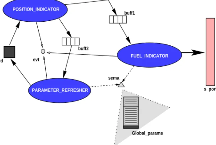
buff2 buff1 board s_port sema evt Global_params FUEL_INDICATOR POSITION_INDICATOR PARAMETER_REFRESHER
Figure 1. The partition ON FLIGHT.
A presentation of the basic component models (communication and syn-chronization services, ARINC processes, etc.) required for the description of avionics applications has been given in [4]. Here, we show how these models are used to describe avionics applications6. Then, we illustrate how timing
issues are addressed, e.g. to compute worst case execution times on the re-sulting description.
6
The example considered in the following takes its inspiration from a real world avionics application which is currently being modeled.
Informal specification of the application. The application is represented by one partition, called ON FLIGHT. Roughly, its function consists in com-puting the current position and fuel level. A report message is produced in the following format:
[date_of_the_report::height::latitude::longitude::fuel_level]
The partition includes the following objects: a blackboard board, two buffers
buff1and buff2, an eventevt, a semaphoresema, a sampling port7 s_port,
and a resource global_params which contains some parameters. There are three processes.
(i) The process POSITION INDICATOR first produces the report message which is updated with the current position information (height, latitude and longitude). It works as follows:
elaborate the report message and set the current date;
send a request to the process PARAMETER REFRESHER for a refresh-ment of global parameters, via buff2 (in order to be able to update the report message with position informations);
wait for notification of end of refreshment, using evt; read the refreshed position values displayed on board;
update the report message with height, latitude and longitude informations; send the report message to the process FUEL INDICATOR, via buff1;
(ii) The main task of FUEL INDICATOR is to update the report message (produced byPOSITION INDICATOR) with the current fuel level.
if a message is contained in the buffer buff1 then
retrieve this message;
end if
update it with the fuel level information from Global params, via protected access (using sema);
send the final report message via the sampling port s port; re-initialize evt;
(iii) Finally, the process PARAMETER REFRESHER refreshes all the global parameters used by the other processes in the partition.
if a refresh request arrives in the buffer buff2 then
retrieve this message;
end if
refresh all the global parameters in Global params, using protected access; display refreshed position values on board;
notify the end of the refreshment, using evt;
Now, let us describe the associated synchronous model.
The Signal model of the partition. The executable model of a partition 7
A sampling port allows no message queuing. There are two kinds of ports: source and destination. A message remains in a source port until it is transmitted by the channel or overwritten by a new occurrence of the message. During transmissions, channels ensure that messages leave source ports and reach destination ports in the same order. A received message remains in the destination port until it is overwritten.
consists of three basic components: first, the executive units represented by ARINC processes; second, the interactions between processes expressed via APEXservices; and finally, the partition-levelOSwhich is in charge of resource allocation to processes within the partition.
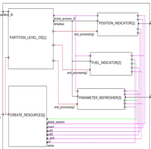
Active_partition_ID initialize report1 report2 end_processing1 POSITION_INDICATOR{1} end_processing2 FUEL_INDICATOR{2} end_processing3 PARAMETER_REFRESHER{3} global_params board buff1 buff2 s_port evt sema CREATE_RESOURCES{} Active_process_ID timedout PARTITION_LEVEL_OS{1}
Figure 2. ASignal model of the partition ON FLIGHT.
The model of the partition ON FLIGHT is shown in Figure 2. We clearly distinguish the partition-level OS as well as the three processes. The box that contains the Signal process CREATE_RESOURCEShas been added for struc-turing. It provides the processes with communication and synchronization mechanisms (e.g. buff1, sema). These mechanisms are created on the occur-rence of the input signal initialize. The presence of this signal corresponds to the initialization phase of the partition. The input Active_partition_ID
represents the identifier of the running partition selected by the module-level OS8, and it denotes an execution order when it identifies the current parti-tion. Whenever the partition executes, the partition-level OS designates an active process within the partition. This is represented by its output signal
Active_process_ID. It is sent to all the processes. Every process that
com-pletes notifies the OS through a special signal (e.g. end_processing1 for the process POSITION_INDICATOR), so the OS can take a decision about the next process to execute.
A process can be blocked during its execution, for instance, when it tries to send a message to a full buffer. A time counter may be initiated to wait for the availability of space in the buffer. The signal timedout produced by the partition-level OSnotifies processes of the expiration of their associated time counters.
8
The activation of each partition depends on this signal. It is produced by the module-level OS which is in charge of the management of partitions in a module.
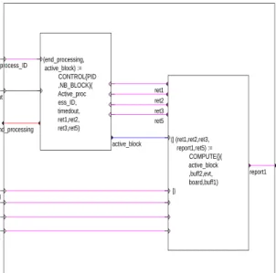
Active_process_ID timedout board buff1 buff2 evt report1 end_processing active_block (end_processing, active_block) := CONTROL{PID ,NB_BLOCK}( Active_proc ess_ID, timedout, ret1,ret2, ret3,ret5) ret1 ret2 ret3 ret5 report1 (| (ret1,ret2,ret3, report1,ret5) := COMPUTE{}( active_block ,buff2,evt, board,buff1) |)
Figure 3. ASignal model of the process POSITION INDICATOR.
Modeling of processes. To illustrate the description of processes, we mainly focus on the process POSITION INDICATOR (the modeling of the other pro-cesses follows the same scheme).
A well-known design principle for getting modularity consists in splitting the considered system into control and computation parts. Among others, one can note the great popularity gained by this idea in hardware design. The model we propose for ARINC processes relies on this principle. So, two ba-sic sub-components are distinguished as shown in Figure 3: CONTROL and
COMPUTE. The former specifies the execution flow of the process. Typi-cally, it is a finite state machine that indicates which statements (or actions) should be executed whenever the process is active. The latter describes these statements grouped into blocks. Each block is attached to a state specified in
CONTROL. The way the two sub-components of the process model interact is similar to what happens in a mode-automaton [11]. On the other hand, a block is assumed to be executed without interruption, within a bounded amount of time.
In the model in Figure 3, the signal active_block identifies a block
se-lected in CONTROL. This block is executed instantaneously. Therefore, one must take care of what kinds of statements can be put together in a block. Two sorts of statements can be distinguished: those which may cause an inter-ruption of the running process (e.g. aSEND BUFFERrequest on a full buffer), termed system calls (in reference to the fact that they involve the partition-level OS); and statements that never interrupt a running process (typically data computation functions), referred to as functions. Since a block is sup-posed to be non-interruptible, we impose that it contains either one system call or one or more functions. This way, the instantaneousness of the block execution is guaranteed to be coherent with its non-interruptibility.
buff2 evt board buff1 ret1 ret2 ret3 report1 ret5 active_block report
(| trigger0 := when (active_block=0) | report := SET_DATE{}(when trigger0) |)
ret1
(| trigger1 := when (active_block=1)
| ret1 := SEND_BUFFER{1}((var buff2) when trigger1,99999.0,2,10.0) |)
ret2
(| trigger2 := when (active_block=2)
| ret2 := WAIT_EVENT{1}((var evt) when trigger2,20.0) |)
d_area d_size ret3
(| trigger3 := when (active_block=3)
| (d_area,d_size,ret3) := READ_BLACKBOARD{1}(... when ...,2.0) |)
ret5
(| trigger5 := when (active_block=5)
| ret5 := SEND_BUFFER{1}((var buff1) when trigger5,var report. Message_Area,var report.Message_Size,10.0) |)
(| trigger4 := when (active_block=4)
| report1 := COMPUTE_POS{}((var report) when trigger4,(var diag_area) when trigger4,(var diag_size) when trigger4) |) t1 t1 t1 t1 t1 t2 t2 t1 t2 t1 t2 block4 block5 block0 block3 block2 block1
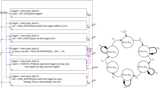
Figure 4. The COMPUTE sub-component and the automaton associated with the CONTROL for the process POSITION INDICATOR.
Figure 4 shows statements contained in COMPUTE. Blocks are represented by inner boxes. The statements associated with a block k are executed when-ever the current state of the automaton specified in CONTROL is blockk, i.e. whenever the event triggerk is present. For instance, from top to bottom, the first block contains a function SET_DATE which produces an instance of the report message, where only the field date_of_the_reportis updated. The other fields will be completed later. The second block contains the system call
SEND_BUFFER, which is used to send a message inbuff2. Input parameters are the message address and size (respectively, denoted by 99999.0 and 2), and a time-out value (10.0 time units) to wait for space when the buffer is full. A return coderet1is sent for diagnostic. Blocks are computed sequentially from
top to bottom as represented by transitions labeled by t1 in the automaton
depicted by Figure 4. However, there could be consecutive executions of a same block. This happens when a system call is executed and the required resource is not yet available. For example, consider the READ_BLACKBOARD re-quest (used to get a message fromboard), if no message is currently displayed in the blackboard, the calling process will get suspended on this block. After a message is available, the process is switched to the “ready” state. As soon as it becomes active, it should re-execute the same block (which induced its suspension) to read the latest message available in the blackboard. These sit-uations are expressed by transition t2 in the automaton.
Modeling of the partition-level OS. The main task of the partition-level OS is to ensure a correct concurrent execution of processes within the parti-tion. Its modeling requires on the one hand, APEX services (e.g. in Figure 5,
CREATE_PROCESSandSTARTare used respectively to create and start processes), and implementation-dependent functions on the other hand, for instance to
define a scheduling policy (e.g. PROCESS_SCHEDULINGREQUESTin Figure 5).
(| (att1,att2,att3) := GET_PROCESSES_ATTRIBUTES{}(when initialize) (a) | (pid1,return_code1) := CREATE_PROCESS{}(att1 when initialize) (b) | (pid2,return_code2) := CREATE_PROCESS{}(att2 when initialize)
| (pid3,return_code3) := CREATE_PROCESS{}(att3 when initialize)
| return_code4 := SET_PARTITION_MODE{}(#NORMAL when (^return_code3)) (c)
| return_code5 := START{}(pid1) (d)
| return_code6 := START{}(pid2) | return_code7 := START{}(pid3)
| partition_is_running := (Active_partition_ID = Partition_ID) (e) | diagnostic := PROCESS_SCHEDULINGREQUEST{}(
when partition_is_running) (f) | (Active_process_ID,status) := PROCESS_GETACTIVESTATUS{}() (g)
| timedout := UPDATE_COUNTERS{}() (h)
| Active_process_ID ^= timedout ^= when partition_is_running | return_code8 := SUSPEND{}(Active_process_ID when (end_processing1
^+ end_processing2 ^+ end_processing3)) (i) | return_code9 := SET_PARTITION_MODE{}(#IDLE when (^end_processing2)) (j) |)
Figure 5. The partition-level OS model.
Figure 5 shows a partial view of the Signal description of the partition-level OS. On the presence of the signalinitialize (which corresponds to the initialization phase of the partition), process attributes are first defined in equation (a), example of attributes are priority, periodicity. Just after that, processes are created9 and started10. For instance, the lines(b)and(d)
cor-respond to the creation and starting of the process identified by pid1 (in fact
POSITION_INDICATOR). In equation (c), the partition is set to the NORMAL
mode11. The signalActive_partition_IDrepresents the identifier of the
run-ning partition selected by the module-level OS. It denotes an execution order when it identifies the current partition, this is the meaning of the boolean
partition_is_running definition (e). So, process rescheduling is performed
whenever the partition is active (see (f)), and the process with the high-est priority in the ready state is designated to execute (Active_process_ID
in equation (g)). On the other hand, all time counters used in the parti-tion are updated whenever it executes (equaparti-tion (h)). The signal timedoutis sent to processes to notify them a possible expiration of their associated time counters. A running process gets suspended as soon as it completes (one of the signalsend_processing1,end_processing2, orend_processing3is received from processes in the partition). This is expressed in equation (i). Finally, 9
Creation [3] does not imply dynamic memory allocation, it only creates a link between the given name and a statically allocated process (this is done via a service called PRO-CESS RECORD in our library) with a suitable stack area having the same name.
10
TheSTART service only puts the specified process in the “ready” state, the process does not execute yet.
11
There are four operating modes [3]: in theIDLEmode, the partition is not executing any process within its allocated windows; in theCOLD START mode, the partition is executing a cold start initialization; in the WARM START mode, the partition is executing a warm start initialization; and in theNORMALmode, the scheduler is activated. All the required resources in the partition must have been created before.
the partition is set to IDLE mode when no process executes while the parti-tion is still active (line (j)). Here, the processFUEL_INDICATORcompletes the last, and notifies the partition-levelOSby sending the signalend_processing2. The above small example aimed to show the feasibility of describing avion-ics applications using the synchronous language Signal. Modularity and ab-straction are key features of the Signal programming. They allow for the scalability of our approach. The description of a large application is achieved with respect to a well-defined design methodology which consists in specifying either completely or partially (by using abstractions) sub-parts of the appli-cation. After that, the resulting components can be composed to obtain new components. These components can be also composed and so on, until appli-cation is complete.
A great advantage of Signal-based modeling is the possibility to formally an-alyze specifications. In particular, timing issues such as worst case execution times, can be addressed using the performance evaluation technique imple-mented in Polychrony.
5
Performance evaluation
A Signal process that models an application is recursively composed of sub-processes, where elementary sub-processes belong to the language kernel and calledatomic nodes. A profiling of such a process substitutes each signal with a new signal representing availability dates date xand automatically replaces atomic nodes with their timing model counter-part (“timing” morphism). The resulting time model is composed (by standard synchronous composition) with the original functional description of the application, and for each signal x, a synchronization with the signal date x is added. The resulting process is close to (or even represents exactly) the model of the temporal behavior of the application running on its actual architecture. One can obviously design less strict modeling to get faster simulation (or formal verification); it is sufficient to consider more abstract representations either of the architecture or of the program.
5.1 Temporal interpretation of Signal processes
An interpretation of aSignalprocess is a process that exposes a different view of the initial one. The structure of the interpretation process is essentially the same but its computations exhibit another aspect of its behavior. The temporal interpretation exposes the time aspect and allows to see how an implementation of a specified function will behave over time [10].
For each process independent of its complexity level, another process can be automatically derived to model its temporal behavior on a given imple-mentation. These processes are called temporal interpretations. For a Signal processP, its temporal interpretation for an implementationI will be denoted
by T(PI), where PI is the Signal process that models implementation I of P. Thus, if a system specified by a processP has a variety of possible implementa-tions I(1)toI(k), then each implementation can be modeled byPI(i), i∈[1, k], and for each PI(i) a temporal interpretationT(PI(i)) can be derived. This way,
a comparative performance evaluation of the different implementations can be performed and the design space of possible implementations can be effectively explored before committing the design to one particular implementation. Such an approach permits to concentrate the design effort to a set of candidate im-plementations.
Signal availability dates. For each signal in the initialSignal specification a date signal is defined in its temporal interpretation: x∈P →T(x)∈T(P). For any signal xinP we have adate xinT(P)withxsynchronous todate x:
P →T(P), x→T(x) =date x, xˆ= date x.
These date signals are some sort of time-stamps providing the availability times for the values of the corresponding signals in the functional specifica-tion, in respect to a global time reference. Depending on the implementation context, time can be measured using either physical time units or full clock cycles. In the first case the date signals are positive real numbers and in the second positive integers. From a cycle count integer measurement we can go on to physical time measurement by multiplying the cycle count to the cycle period.
Each operation in a Signal specification is represented by a node in the Hierarchical Conditional Dependency Graph, which is the internal represen-tation of a Signal program. To each node in the graph, a delay is associated. This delay is represented by the same data type as the data type used to represent dates and is a function of several parameters. The actual node de-lay is obtained by giving values to these parameters. The dede-lay depends on parameters like: the operation performed by the node, data types involved, the chosen implementation, etc. Furthermore, a delay can be represented by a pair of numbers corresponding to the worst and best case delays. Since delays are represented by intervals, dates will be represented as intervals too. Com-puting these dates takes into account the processing delays. It is important to note that this date mechanism allows us to go from logical to physical time.
Non-functional interpretations. The temporal interpretation of aSignal specification is just a special case of a general non-functional interpretation. The non-functional interpretations are Signal processes and as such they can be decomposed into a control and a data part. The control computations are identical to those in the initial processes from which the interpretations are derived. What changes are the data computations since they extract the information related to the particular interpretation.
For a Signal process P we know that P = CP|DP, with CP and DP rep-resenting respectively the control and data parts of P. Similarly for an inter-pretation of P, we have: T(P) = CT(P)|DT(P). Since the interpretation of a complex process can be defined as the recursive composition of the
interpre-tations of the constituent processes for T(P) we have: T(P) =T(CP)|T(DP), with T(CP) =CT(CP)|DT(CP) and T(DP) =CT(DP)|DT(DP).
For the control part, we have CT(P)=CP.
Ib Ib T(I) H OD B ID H B O T(O) O I H DT(P) CP P CP P T T(P) D
Figure 6. Temporal interpretation of a Signalprocess P.
The process of obtaining an interpretation T(P) of a process P is graphi-cally depicted in Figure 6. This process gives a general form of morphism of Signalprograms, which is available inPolychrony. The data part (DP) of the process P computes output values (OD) from input values (I). The computa-tions are conditioned by activation events (H) computed in the control part (CP). To compute the activation conditions H, CP uses Boolean input signals (Ib) and intermediate Boolean signals B computed by DP. Finally, certain outputs are output events (HO) computed by CP. The control parts of the initial process and its interpretation are identical, but the data computations differ. The data computations in T(P) extract the information of interest, implicit in the initial specification P.
The date computation model. The Signal kernel operators are the sim-plest processes that can be used to build more complex ones. Similarly, the interpretation of a process can be viewed as the composition of the interpre-tations of the primitive processes making up the initial process.
The interpretations of the kernel processes perform the appropriate com-putations relating to a particular interpretation. These interpretations are organized in a collection which represents the library of cost functions, de-fined in Signal. For each interpreted process, this library is extended with the interpretations of external function calls and other separately compiled processes, used in the initial process. For example, the “timing” morphism available in Polychrony associates with the monochronous addition operator
z := x + y, the following cost function:
process CostPlus{type_x, type_y}
( ? date_type date_x, date_y, date_clk_z, wait_i; ! date_type date_z, done_i )
(| date_z := MAX2( MAX3( date_x, date_y, date_clk_z), wait_i when ^date_z) + getCostPlus{type_x, type_y}()
| done_i := (date_z default wait_i) cell ^done_i |)
where theMAXndenotes a process that returns the maximum value ofn in-puts, among those that are present at a given instant (it is not monochronous). The notations type x and type y represent respectively the types of x and y;
date clk z is a signal associated with the common clock of x, y and z by the morphism. Signals wait i and done i are associated with the current node and have the same type as date signals: wait i accumulates dates coming from incoming precedences other than data dependencies, whereas done iis a date required by the next nodes other than data dependencies (i.e. done i is part of wait i+1). The date of z, denoted by date z, is the sum of the max-imum date of inputs and the delay of the addition operation, some ∆+. The
quantity ∆+ depends on the desired implementation, on a specific platform.
It has to be provided in some way by the user, with respect to the considered architecture. In the current implementation in Polychrony, the value ∆+ is
provided by a function getCostPlus which has the types of the operands as parameters and which fetches the required value from some table.
The scheme illustrated above for monochronous operators handles also “control” operators. For constructs such as the defaultoperator, which allow for control branching, the definition of the associated interpretation accounts for this branching (for a default b, the date at which the input value is available is given by date a default date b). Moreover, thanks to composi-tionality of Signal specifications, the above mechanism can be applied at any level of granularity.
5.2 Obtaining results
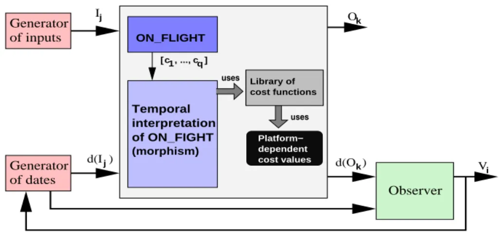
Figure 7 depicts a co-simulation of the application model composed with its associated temporal interpretation. At each iteration, the date of an output (d(Ok)) depends on the date of an input (d(Ij)) and thecontrol configuration represented by a “valuation” of a condition vector [c1, . . . , cq] corresponding to intermediate boolean signals B (cf. Fig. 6) computed in the original pro-gram. In a straightforward approach, it is possible to provide a set of vectors that covers all the possible combinations for the control flow. A better way is to take into account the existing relationships between these booleans such as provided by the clock calculus (this is expressed through the composition of the original program and its temporal interpretation). In addition, specific
observer processes, comparing dates or verifying some conditions (timing
re-quirements) for example, can be inserted into the model.
Comments. Execution time estimation is an important metric for per-formances in real-time system design. Some current practices for timing pre-dictability proceed by actually running programs on a set of test data and measuring execution times. One major drawback here concerns the degree of pertinence of this set of data w.r.t. the considered context. Other approaches such as [13] [12] have shown that timing issues can be successfully addressed at higher level languages (e.g. language C) rather than lower level languages (e.g. assembly language). In the case of the Signal language, the timing pre-dictability problem consists in simulating aSignal program which reflects the temporal dimension of an initial program. On the other hand, the tools and
O V d(I ) Generator Observer I of inputs Generator of dates d(O ) Temporal (morphism) j of ON_FIGHT i interpretation k j k c cost functions Library of [ , ..., ]1 q ON_FLIGHT c uses uses Platform− cost values dependent
Figure 7. Co-simulation of the application with its temporal interpretation. techniques available in Polychrony remain applicable on this temporal “im-age” (e.g. for the purpose of some formal verifications when the corresponding required abstractions are considered).
Several successful experiments have been done on sampleSignalprograms. For the ON FLIGHT model, some simplifications have been made because of the complexity of used data structures. So, the cost of the accesses to those data structures and related effects is not taken into account. The cost func-tion library currently considers simple data structures (e.g. integer, boolean, arrays). Others are considered as external. As a result, the current computed results are not relevant enough to be highlighted here. However, this library is being currently enhanced to allow more efficient experiments on programs with complex data structures. Thus, more relevant results will be available soon.
6
Conclusions
In this paper we illustrated an approach to the modeling of avionics applica-tions for the purpose of formal verification and analysis. The whole approach relies on the use of a single formalism of the Signallanguage. This is part of a more general design methodology for distributed embedded applications, de-fined within Polychrony. This methodology proceeds by successive transfor-mations on an initial Signalmodel that preserve semantic properties. During the transformations, “abstract” components can be instantiated in different ways from modules related to actual target architecture features, address-ing various purposes (embedded code generation, temporal validation, etc.). We considered models of APEX services [4] to describe avionics applications. Then, we used the Polychrony tool-set to analyze applications, in particular, we focused on the real-time behavior. The technique [10] is still being im-plemented in order to take into account Signal programs with complex data structures (such as the model of the partition ON FLIGHT described in this paper).
References
[1] A. Benveniste and G. Berry, The Synchronous approach to Reactive and Real-Time Systems, proc. of IEEE, vol. 79, No. 9, pages 1270-1282, April 1991.
[2] E. Closse, M. Poize, J. Pulou, J. Sifakis, P. Venier, D. Weil, and S. Yovine, TAXYS: a tool for the development and verification of real-time embedded systems, proc. of Computer Aided Verification, Paris, France, Springer-Verlag, July 2001.
[3] Airlines Electronic Engineering Committee, ARINC Specification 653: Avionics Application Software Standard Interface, Aeronautical radio, Inc., Annapolis, Maryland, January 1997.
[4] A. Gamati´e and T. Gautier, Modeling of Modular Avionics Architectures Using the Synchronous Language Signal, In the 14th Euromicro Conference on Real Time Systems, WiP session, IEEE Press, June 2002. (Complete version is available as INRIA research report n. 4678, December 2002).
[5] A. Gamati´e and T. Gautier, The Signal Approach to the Design of System Architectures, In the 10th IEEE International Conference and Workshop on the Engineering of Computer Based Systems, April 2003.
[6] T. Gautier and P. Le Guernic,Code generation in the SACRES project, Safety-critical Systems Symposium, Springer, Huntingdon, UK, February 1999.
[7] P. Le Guernic, T. Gautier, M. Le Borgne, and C. Le Maire, Programming real-time applications with Signal, in proc. of IEEE, 79(9), p. 1321-1336, September 1991. [8] D. Goshen-Meskin, V. Gafni and M. Winokur,Safeair: An Integrated Development
Environment and Methodology, INCOSE’01, Melbourne, July 2001.
[9] T. A. Henzinger, B. Horowitz and Ch. Meyer Kirsch, Embedded Control Systems Development with Giotto, proc. of LCTES. ACM SIGPLAN Notices, 2001.
[10] A. Kountouris and P. Le Guernic,Profiling of SignalPrograms and its application in the timing evaluation of design implementations, proc. of the IEE Colloq. on HW-SW Cosynth. for Reconfig. Systems, p. 6/1-6/9, HP Labs, Bristol, UK, February 1996. [11] F. Maraninchi and Y. R´emond,Mode-Automata: About Modes and States for Reactive
Systems, European Symposium On Programming, Lisbon, Portugal, Springer-Verlag, March 1998.
[12] C. Y. Park and A. C. Shaw,Experiments with a Program Timing Tool Based on Source-Level Timing Schema, IEEE Computer 24(5): 48-57, May 1991.
[13] P. Puschner and Ch. Koza,Calculating the Maximum Execution Time of Real-Time Programs, Journal of Real-Time Systems, vol 1, n. 2, p. 159-176, September 1989. [14] J. Sifakis, Modeling Real-Time Systems - Challenges and Work Directions,
EMSOFT’01, Tahoe City. Lecture Notes in Computer Science 2211, October 2001. [15] S. Vestal,MetaH Support for Real-Time Multi-processor Avionics, IEEE Workshop on