ARTICLE TEMPLATE
A semiparametric copula-based estimation of the regression function for right-censored data
Taoufik Bouezmarnia, Yassir Rabhib and Charles Fontainec
aDepartment of Mathematics, University of Sherbrooke, Sherbrooke Canada. Centre interuniversitaire de recherche en ´economie quantitative (CIREQ). Email:
[email protected];bState University of New York, Cortland, USA. Email: [email protected];c Institut Universitaire de Recherche Clinique, Universit´e de Montpellier 641, Ave du Doyen Gaston-Giraud 34090 Montpellier France. Email:
ARTICLE HISTORY
Compiled September 20, 2019
ABSTRACT
This paper addresses the semiparametric estimation of the regression function in a situation where the response variable is right-censored and the covariate(s) is com-pletely observed. We present a new copula-based method to estimate the regression function. The key concept presented in this manuscript is to write the regression function in terms of the copula density and marginal distributions. We suppose a parametric model for the copula density with unknown parameter(s) and we estimate the marginal distributions of the response and the covariate by the Kaplan-Meier estimator and the empirical distribution, respectively. We establish the asymptotic properties of our estimator and extend it to the multivariate case. The proposed method is then applied to analyze a data-set on lifetime with lung-cancer.
KEYWORDS
Semiparametric copula-based estimation; Regression function; Censored data; Parametric copula models; Kaplan-Meier estimator.
1. Introduction
Incident cohort design is usually adopted to study the time between an initiating event, say disease onset, to a terminating event, say death. The failure times of individuals recruited in such studies may however be subject to right-censoring due to voluntary retraction, emigration or end of study. Right-censoring on the response variable (failure time) arises when the followed subjects in a study cannot provide us information on the outcome of the study despite of our knowledge of the predictors for these subjects (e.g. age at disease onset).
The relation between these predictors and the response variable is one of the most
This work has been supported by the Natural Sciences and Engineering Research Council of Canada (NSERC), Canssi and Statlab-CRM (Canada) and Le Fonds de recherche du Qu´ebec (Nature et technolo-gies). The authors thank Prof Alexander Meister (the editor), the associate editor, and two referees for their helpful and constructive comments.
important problem in statistics. In particular, the regression model Y =m(X) +ε,
where m(x) = E[Y|X = x] is an unknown smooth function and ε is a random error (E[ε|X = x] = 0 and E[ε2|X = x] < ∞). The estimation of the regression function m have been extensively studied in literature under different data settings. At first, [18] and [11] proposed estimators based on the linear regression model with some methodological weaknesses since they both require a particular censoring pattern. Furthermore, based on the general linear model, the method proposed by [1] is an iterative sequence of estimators and has the drawback of not necessarily converging. In the work of [5,13,24,26–28], data transformations for censored data were presented. The problem with the linear regression models is that they are too restrictive. Nonparametric methods, for example Nadaraya-Watson or local linear kernel (see [6]), provide a flexible method, since they do not assume a specific model for the regression function. However, the nonparametric approaches suffer from the curse of dimensionality. More recently, several copula-based methods were proposed to estimate m for complete data. For instance, see the parametric approach of [25], [12] and [3], and the semiparametric method of [20].
Consider a response variableY, with distribution F0 and density f0, and a vector
ofdpredictorsX = (X1, ..., Xd) with joint distributionFX and joint densityfX. Let F1, . . . , Fd be the respective marginal distributions of X1, . . . , Xd, x = (x1, . . . , xd) and denoteF(x) = F1(x1), . . . , Fd(xd)
. From the copula theory, it is known that the multivariate distributionFY,X1,...,Xd is given by
FY,X1,...,Xd(y, x1, . . . , xd) =C(F0(y), F1(x1), . . . , Fd(xd)),
where C is the copula distribution of (Y, X1, ..., Xd) with uniform margins on [0,1].
Using this decomposition, the conditional density of Y given X = x can be written in terms of copula densities as
fY|X=x(y) =f0(y)
c(F0(y),F(x))
cX(F(x))
, (1)
wherec andcX are the respective copula densities of (Y, X1, ..., Xd) and (X1, ..., Xd). Using a copula-based parametric approach, [25], [12] and [3] investigated the re-lationship (1) for various copula families (e.g. Gaussian, Student, Farlie-Gumbel-Morgenstern (FGM), Iterated FGM, Archimedean) in order to estimate the regres-sion function m(x) for single and multiple covariates. For instance, if the copula density of (Y, X1) belongs to the FGM family with parameter θ, i.e. c(u0, u1) =
1 +θ(1−2u0)(1−2u1), then
m(x1) =E[Y] +θ(2F1(x1)−1) Z
F0(y) (1−F0(y)) dy.
For the multiple covariates case (d≥2), see [12]. Note that for θ = 0 Y and X1 are
then m(x) =E F0−1 Φ uTΣ−X1ρ+Z q 1−ρTΣ−1 Xρ ,
where u = (Φ−1(F1(x1)), . . . ,Φ−1(Fd(xd)))T, ρ = (corr(Y, X1), . . . , corr(Y, Xd))T,
Z ∼ N(0,1), Φ is the standard normal cdf and ΣX is the correlation ma-trix of X. For ρ = 0, Y and X are independent and m is simplified to m(x1) = E
F0−1(Φ(Z)) ≡ E[Y]. A semiparametric approach was taken re-cently by [20] to estimatemfor complete data. The latter assume a parametric model for the copula density and estimate the marginal distributions using nonparametric methods.
In this paper, we propose a semiparametric copula-based estimator for the regres-sion function when the response variable is subject to right-censoring. Here, we assume a parametric model for the copula density and we propose to estimate the marginal distributions F0 by the product-limit estimator and F1, . . . , Fd by their empirical counterparts. To the best of our knowledge, such method has never been proposed or studied in the literature. Assuming a parametric model for the copula density avoids the curse of dimensionality but requires the choice of the adequate copula model. The paper is organized as follows. In Section 2, we define our estimator for the regression function in the case of right censored data. In Section 3, we establish the asymptotic properties of the proposed estimator by providing its i.i.d. representation, and showing its uniform weak convergence and asymptotic normality. In section 4, we apply our methodology to analyze a data-set on lifetime with lung-cancer. The proofs of the theoretical results are presented in the appendix.
2. Estimator for right-censored data
Suppose that the response Y is subject to right-censoring by a random variable C and one observes the vector (Z, δ) = min(Y, C),I(Y ≤C), where δ indicates if Y is censored or not. We assume thatY andCare independent and we consider uncensored covariates X1, . . . , Xd. The data has the form
Zi, δi, X1,i, . . . , Xd,i
, i= 1, . . . , n . Based on the relationship (1), the regression function m(x) = E[Y|X =x] can be
expressed in terms of the copula density and the marginal distributions as
m(x) =E h Y w F0(Y),F(x) i = e(F(x)) cX(F(x)) , (2)
wherew(u0,u) =c(u0,u)/cX(u) and
e(u) =
Z 1 0
F0−1(u0)c(u0,u) du0,
with F0−1 the inverse of F0. In the particular cases of a single covariate (d = 1) or
Formula (2) allows different ways for estimatingm. One approach assumes a para-metric model for the copula densities and the marginal distributions. The parameters of the copula density and those of the marginal distributions can be estimated by using maximum likelihood (ML) or inference functions for margins method ((IFM)) in two steps [see [23] and [9]]. The IFM method provides results similar to that of maximum likelihood (ML) and is easier to implement This method is however too restrictive, and a misspecification of the parametric model leads to wrong conclusions. A second way is to estimate nonparametrically the copula density and the marginal distributions. For example, the method proposed by [8] and [2] to estimate the copula density can be adapted to right-censored data. However, this method suffers from the curse of dimensionality and requires practical bandwidth parameters. The third ap-proach is semiparametric. This method considers a parametric model for the copula density and nonparametrically estimates the marginal distributions. The semipara-metric approach is less restrictive than the parasemipara-metric method and avoids the curse of dimensionality of the nonparametric estimator. The estimation of the copula distri-bution based on a semiparametric approach have been proposed by [7], for complete data, and by [23] for right-censored data. Based on extensive simulations, [10] showed that the semiparametric approach outperforms the ML and IFM methods.
To estimate the regression function m, we consider a parametric model c(·,·;θ) for the copula density, where θ is an unknown parameter vector, and nonparametric estimators forF0andFj (j= 1, . . . , d). First, the marginal distribution of the response is replaced by the Kaplan-Meier estimator, Γn, defined as follows :
Γn(t) = 1− Y 1≤i≤n Z(i)<t n−i n−i+ 1 δ(i) ,
where Z(1), . . . , Z(n) are the ordered responses and δ(1), . . . , δ(n) their respective con-comitant censoring indicators. The marginal distributions of the covariates are esti-mated by the rescaled empirical distributionFbj(t):
b Fj(t) = 1 n+ 1 n X i=1 1(Xj,i ≤t),
withXj,1, . . . , Xj,n i.i.d random copies ofXj (j = 1, . . . , d).
Then, we estimate the copula parameter θ by the estimator ˆθ that maximises the pseudo maximum likelihood given in equation (11) of [23]. Therefore, an estimator for the numeratore(F(x)) is
ˆ e(Fb(x)) = n X i=1 Ziwic(Γn(Zi),Fb(x);θ),b (3) where Fb(x) = Fb1(x1), . . . ,Fbd(xd)
and wi is the mass attached to Zi under the Kaplan-Meier estimator, i.e., w1 = Γn(Z(1)) and wi = Γn(Z(i)) −Γn(Z(i−1)), i =
2, . . . , n. Now, using the fact thatcX(u) =E
h
c F0(Y),u i
denomi-natorcX(F(x)) by b cX(Fb(x)) = n X i=1 wic(Γn(Zi),Fb(x);θ),b (4)
Thus, our semiparametric estimator form(x) is
b m(x) = e(ˆFb(x)) b cX(Fb(x)) = n X i=1 Zi wic(Γn(Zi),Fb(x);bθ) Pn i=1wic(Γn(Zi),Fb(x);θ)b . (5)
In the particular case of a single covariate (d= 1), or mutually independent predictors X1, . . . , Xd, the estimator of m(x) is reduced to
b m(x) = n X i=1 Ziwic(Γn(Zi),Fb(x));θ).b (6)
LetL(z) =P[Z ≤z] andτ = sup{z: L(z)<1}<∞. Since the tail region information on the survival function ofY may not be identifiable in [τ,∞) due to right censoring, we note that Γn is defined on the interval [0, τ].
Remark 1.
1.We can consider other estimators,Γne andFje (j= 1, . . . , d), to estimate the response
and marginal distributions provided that the following conditions are satisfied : (i) eΓn(t) = Γn(t) +op(n−1/2).
(ii) Fej(t) =Fbj(t) +op(n−1/2), forj= 1, . . . , d.
2.The model in (2) can be extended to mixed (continuous and discrete) covariates. However, this model can’t be used for a discrete response. The idea proposed in [4], for complete data, can be adapted to our model by assuming a latent variable framework to describe discrete outcomes.
3. In the case where some of the predictors are subject to right-censoring, we may estimate their distributions by the Kaplan-Meier estimator instead.
4.The nonparametric kernel estimator (Nadaraya-Watson type)
b mNP(x) = n X i=1 wiKd(x−hX.,i) Pn `=1w`Kd(x −X.,` h ) Zi,
with Kd a kernel function defined on Rd and h the smoothing parameter, is a
robust alternative to our semiparametric estimator. This estimator requires less assumptions and is more flexible. However, the a.s. convergence rate of mb
NP is Oa.s. n−1log(n)1/(d+2) in the presence of d covariates. This rate becomes slower as the dimension of the covariates increases.
3. Asymptotic results
We start by presenting some notations and assumptions, on the copula and its parameters, needed for establishing the asymptotic properties of the regression function estimator. Denote ∂jc=∂c/∂uj for j = 0, . . . , d, ˙c = (∂c/∂θ1, . . . , ∂c/∂θp)T and letx∈Rdsuch that F(x)∈(0,1)d.
Assumption A: Let g be either c, ˙c or∂jc (j= 0, . . . , d).
(i) (u, θ) → gu0(u, θ) ≡ g(u0,u;θ) is continuous at (F(x), θ0), uniformly on u0 ∈
[0,1].
(ii) u0 →g(u0,F(x);θ0) is continuous on [0,1].
Assumption B:The parameter estimator θbsatisfies,
b θ−θ0= 1 n n X i=1 ζi+op(n−1/2),
whereζi are i.i.d. random variables with zero mean and finite variance.
As noted above, we consider the estimation ofθ proposed by Shih & Louis (1995) for a bivariate parametric copula model. This estimator satisfies Assumption B, and by a similar approach, we may extend the latter representation to a multivariate parametric copula model (d >2).
Assumption C:
The copula density is bounded and bounded away from zero on its compact support. The copula densitycis required to be bounded away from 0 for a regression model with multiple covariates. All the parametric copula densities (Gaussian, Student, Archimedean copula, etc) are bounded away from zero. These densities are bounded on (0,1)d, but some of them are unbounded at the corners of [0,1]d. To relax Assump-tion C, the proofs in the appendix can be adapted by considering a copula density that satisfies the condition
c(u0, u1, ..., ud) =O 1 q Qd j=0uj(1−uj) .
This condition is satisfied by many common copula densities (see [21]).
3.1. Main results
We begin by considering the case of one covariateX1 (d= 1). In Proposition 3.1, we
establish the uniform weak convergence of the proposed regression function estimator
b
m. The i.i.d. representation ofmb is derived in Theorem 3.2, while in Corollary 3.3, the
Proposition 3.1. Under Assumptions A and B we have sup x1 m(xb 1)−m(x1) =Op p n−1log logn .
Proof. The proof is given in the appendix.
Denote
ηi,1(x1) = Z τ
0
y ξi(y)∂0c(F0(y), F1(x1);θ0) dF0(y),
ηi,2(x1) = I(X1i≤x1)−F1(x1) Z τ 0 y ∂1c(F0(y), F1(x1);θ0) dF0(y), ηi,3(x1) = Z τ 0
y ζic(F˙ 0(y), F1(x1);θ0) dF0(y),
ηi,4(x1) = Z τ
0
ξi(y) dHx1(y),withHx1(y) =yc(F0(y), F1(x1);θ0).
withξi(y) the i.i.d. random term of the representation of the Kaplan-Meier estimator Γn, see [14]. The additional terms ηi,1, ηi,2 and ηi,4 are needed because the marginal
distributions are estimated in the first step.
Theorem 3.2. Let ηi =P4j=1ηi,j. Under Assumptions A and B,mb admits the i.i.d. representation b m(x1) =m(x1) + 1 n n X i=1 ηi(x1) +op(n−1/2) (7)
The proof is is given in the appendix. The representation of mb in (7) leads to the
following result.
Corollary 3.3. Under Assumptions A and B, √nm(xb 1)−m(x1)
converges to a
normal distribution with zero mean and varianceσ2(x1) =Eη21(x1)
.
3.2. Extension to the multivariate case
Following similar steps in proof of Proposition 3.1, we can establish the uniform weak convergence, with the same order as in Proposition 3.1, ofmb with multiple covariate.
Next, we extend the result in Theorem 3.2 to the multivariate cased≥2, by following similar arguments in Theorem 3.2’s proof. First, one can easily check that ˆe admits the representation ˆ e( ˆF(x))−e(F(x)) =n−1 n X i=1 ϕi(x) +op(n−1/2), (8)
wherex= (x1, . . . , xd), F(x) = (F1(x1), . . . , Fd(xd)) andϕi =P4j=1ϕi,j, with
ϕi,1(x) = Z τ
0
y ξi(y)∂0c(F0(y),F(x);θ0) dF0(y),
ϕi,2(x) = d X j=1 I(Xji ≤xj)−Fj(xj) Z τ 0 y ∂jc(F0(y),F(x);θ0) dF0(y), ϕi,3(x) = Z τ 0 y ζiTc(F˙ 0(y),F(x);θ0) dF0(y) and ϕi,4(x) = Z τ 0
ξi(y) dHx∗(y) withHx∗(y) =c(F0(y),F(x);θ0).
Second, one can show thatbcX has the representation
b cX( ˆF(x))−cX(F(x)) =n−1 n X i=1 φi(x) +op(n−1/2), (9)
whereφi=P4j=1φi,j, with φi,1(x) =
Z τ
0
ξi(y)∂0c(F0(y),F(x);θ0) dF0(y),
φi,2(x) = d X j=1 I(Xji≤xj)−Fj(xj) Z τ 0 ∂jc(F0(y),F(x);θ0) dF0(y), φi,3(x) = Z τ 0 ζiT c(F˙ 0(y),F(x);θ0) dF0(y) and φi,4(x) = Z τ 0 ξi(y) dHx∗(y). Combining (8) with (9) leads to the next main result. Theorem 3.4. Under Assumptions A, B and C, we have
b m(x)−m(x) =n−1 n X i=1 1 cX(F(x)) h ϕi(x)−m(x)φi(x) i +op(n−1/2).
Theorem 3.4 implies that √n b
m(x)−m(x)
follows asymptotically a normal distri-bution with mean zero and variance
σ2(x) =Var 1 cX(F(x)) h ϕi(x)−m(x)φi(x) i .
−20 0 20 40 60 1 2 3 4 5 6 7 Weight loss logar ithm of Lif etime (da ys)
(a) lifetime vs Weight-Loss.
0 5 10 15 20 25 1 2 3 4 5 6 7 Calories−Meal (x 100) logar ithm of Lif etime (da ys) (b) lifetime vs Calories-Meals.
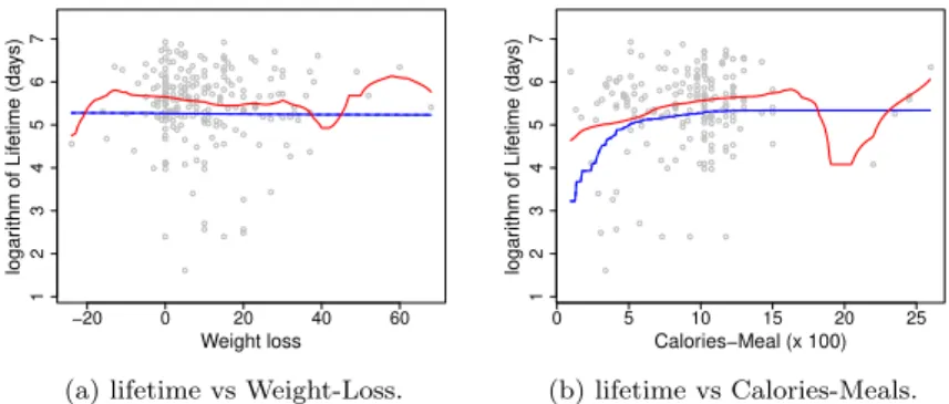
Figure 1. Regression function estimators of patients with lung cancer: (a) lifetime vs Weight-Loss, (b) lifetime vs Calories-Meals. Copula-based estimator (blue line) and nonparametric kernel estimator (red line).
4. Data analysis
4.1. Survival with lung cancer
We illustrate the methodology described in Section 2 by analysing a set of survival data from patients with advanced lung cancer collected by the “North Central Can-cer Treatment Group” (see [16]). The primary goal of [16] was the investigation of whether descriptive information from a patient-completed questionnaire could provide prognostic information that was independent from the one obtained by the physi-cian. The questionnaire (which contains different questions about age, calories intake, weight-loss in the last six months, etc) was completed by the patients before entering the study of lung cancer. This study was mainly focused on dietary and daily activities factors and their possible relation to risk of lung cancer. The data set contains the lifetimes of n = 228 individuals (men and women), among whom 165 died and 63 were right-censored during the follow-up. The survival timeY is defined as the time between onset of lung cancer and death. In this example, we consider two covariates: X1 as the weight loss in the last six months prior to entering the study andX2 as the
average of meal calories per day before entering the study; hence the two covariates are completely observed.
To choose the copula function for our semiparametric regression estimator, we con-sider the copula model {c(.;θ), θ ∈ Θ} that minimizes the weighted sum of squared residuals defined by n X i=1 wi h Zi−mbc(Xi) i2 . (10)
This leads to select the Gaussian and Clayton copulas for estimating the regression functions of Lifetime vs Weight-Loss and Lifetime vs Calories-Meals, respectively. Fig-ure 1 displays the plots of the semiparametric copula-based estimator (blue line) and the nonparametric kernel estimator (red line) defined by
b mNP(x) = n X i=1 wiK x−Xi hn n X `=1 w`K x−X` hn Zi, (11)
10 20 30 40 50 60 0 1 2 3 4
Age at Transplant (years)
logar
ithm of Lif
etime (da
ys)
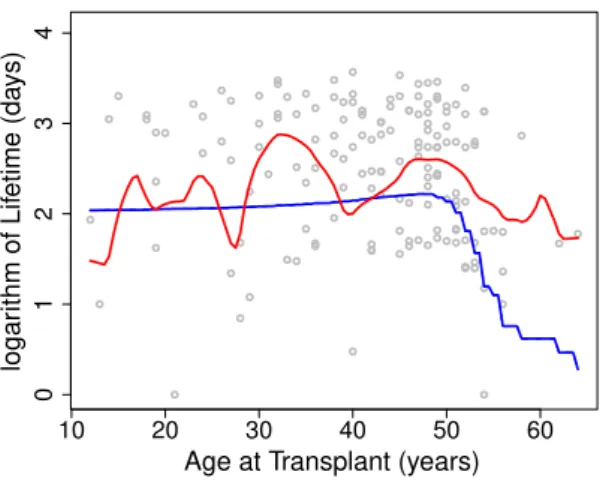
Figure 2. Regression function estimators of 157 heart transplant patients. Copula-based estimator with Joe’s copula (blue line) and nonparametric kernel estimator (red line).
where K(x) = 0.75(1 −x2) I(−1 ≤ x ≤ 1) and hn > 0 is a sequence of band-width tending to 0. Both estimators show similar behaviors and fluctuate about the survival-time e5.3 ≈ 200 days. The horizontal tendency of the copula-based estima-tors can be explained by the weak dependence between the response (lifetime) and the two covariates. In [22], we found that the estimates of Kendall’s tau measure of association is bτY,X1 = −0.0848, for Lifetime vs Weight-Loss, and bτY,X2 = 0.1335,
for Lifetime vs Calories-Meals. This indicates weak association between the response and the covariates. These results concur with the findings of [16]. Note that in (11) we select the bandwidth hn that minimizes the weighted integrated squared error WISE(h) =Rx>0 h b mN P(x;h)−m(x)i2dFX(x), given by b h= arg min h ( n X i=1 wi h b mN P−i (Xi;h)−Zi i2) ,
wherembN−iP(x) is a leave-one-out estimate ofm atx;
b mN−iP(x;h) = n X k=1 k6=i wkK x−Xk h n X j=1 j6=i wjK x−Xj h Zk.
4.2. Heart transplant data
The Stanford survival data were extracted from a program of heart transplant which began in October 1967 (see [19]). The patients had to be selected to take part of that program and therefore received a transplant. Some people die between the selection of
of the study was February 1980, and at this moment, the data about heart transplant of 184 patients was collected. The variables of interest in this analysis are the survival timeY (in days), the failure statusδ (1 if dead and 0 if alive and censored) and the age at the time of the first transplantX. We only keep patients who their mismatch score is not missing. Therefore, we get a sample ofn= 157 data with a censorship of 35%. Figure 2 illustrates the semiparametric copula-based estimator (blue line) and the nonparametric kernel-estimator (red line), given by (11). The copula-based estimator shows a slight increase up to Age-of-Transplant = 50, and then a decrease after that. This indicates a rapid decline in the survival of patients who received a transplant after the age of fifty. The Age-of-Transplat variable (X) seems to have an impact on the survival time (Y). In [22], the estimation of Spearman’s rho measure of association isρbY,X =−0.626. This reflects a moderate strong association betweenX and Y, and concurs with the finding of [19]. Note that we employed the weighted sum of squared residuals defined in (10) to select the Joe copula for this data.
5. Conclusion
We introduced a new copula-based estimator for the regression function when the response variable is subject to right-censoring and the covariate(s) is completely ob-served. The key element in the paper is to write the regression function in terms of the copula density and marginal distributions. The estimation method uses a parametric model for the copula density, with unknown parameter(s), and estimate nonparamet-rically the marginal distributions of the response and covariate(s). We studied the asymptotic behavior of our estimator analytically, and we extend it to the multivari-ate case. The proposed estimation method have shown satisfactory results in analyzing two real data-sets, concerning survival with heart-transplant and lifetime with lung-cancer.
Acknowledgement(s)
This work has been supported by the Natural Sciences and Engineering Research Council of Canada (NSERC), Canssi and Statlab-CRM (Canada) and Le Fonds de recherche du Qu´ebec (Nature et technologies).
References
[1] Jonathan Buckley and Ian James. Linear regression with censored data. Biometrika, pages 429–436, 1979.
[2] S. X. Chen and T. Huang. Nonparametric estimation of copula functions for dependent modeling. Canadian Journal of Statistics, 35:265–282, 2007.
[3] G.J. Crane and J. Van Der Hoek. Conditional Expectation Formulae for Copulas. Aus-tralian and New Zealand Journal of Statistics, 50:53–67, 2008.
[4] A. R. de Leon and B. Wu. Copula-based regression models for a bivariate mixed discrete and continuous outcome. Statistics and Medecine, 30:175–185, 2011.
[5] K. Doksum and B. Yandell. Properties of regression estimates based on censored survival data.In A festschrift for Erich L. Lehmann (eds P. J. Bickel, K. Doksum and J.L. Hodges Jr.), pages 140–156, 1983.
[6] J. Fan and I. Gijbels. Censored-regression: local linear approximations and their applica-tions. Journal of the American Statistical Association, 89:560–570, 1994.
[7] C. Genest, K. Ghoudi, and L.P. Rivest. A semiparametric estimation procedure of de-pendence parameters in multivariate families of distributions. Biometrika, 82:543–552, 1995.
[8] I. Gijbels and J. Mielniczuk. Estimating the density of a copula function.Communications in Statistics - Theory and Methods, 19, 1990.
[9] H. Joe and J. Xu. The estimation method of inference functions for margins for multivari-ate models. Technical Report, Department of Statistics, University of British Columbia, 166, 1996.
[10] G. Kim, M. Silvapulle, and P. Silvapulle. Comparison of the semiparametric and para-metric methods for estimating copulas. Computational Statistics and Data Analysis, 51: 2836–2850, 2007.
[11] H. Koul, V. Susarla, and J. Van Ryzin. Regression analysis with randomly right censored data. Annals of Statistics, 9:1276–1288, 1981.
[12] Yeo Keng Leong and Emiliano A Valdez. Claims Prediction with Dependence using Copula Models. Technical report, 2005.
[13] S. Leurgans. Linear models, random censoring and synthetic data. Biometrika, 74:301– 309, 1987.
[14] S. Lo, Y. Mack, and J. Wang. Density and hazard rate estimation for censored data via strong representation of the Kaplan-Meier estimator. Probability Theory and Related Fields, 80:461–473, 1989.
[15] S.H. Lo, Y.P Mack, and J.L Wang. Density and hazard rate estimation for censored data via strong reptresentation of the kaplan-meier estimator. Probability Theory and Relatd Fields, 80:473–473, 1989.
[16] C.L. Loprinzi et al. Prospective evaluation of prognostic variables from patient-completed questionnaires. North Central Cancer Treatment Group. J. Clin. Oncol., 12:601–607, 1994.
[17] X.L. Meng, Y. Bassiakos, and S.H. Lo. Large-sample properties for a general estimator of the treatment effect in the two-sample problem with right censoring. Ann. Statist., 19: 1786–1812, 1991.
[18] R. Miller. Least squares regression with censored data. Biometrika, 63:449–464, 1976. [19] R. Miller and J. Halpern. Regression with Censored Data.Biometrika, 69:521–531, 1982. [20] H. Noh, A. El Ghouch, and T. Bouezmarni. Copula-Based Regression Estimation and
Inference. Journal of the American Statistical Association, 108:676–688, 2013.
[21] M Omelka, I. Gijbels, and N Veraverbeke. Improved kernel estimation of copulas: Weak convergence and goodnees-of-fit testing. Annals of Statistics, 37:3023–3058, 2009. [22] Y. Rabhi and T. Bouezmarni. Nonparametric inference for copula density function under
random censoring. Technical report, Dept. of Mathematics, University of Sherbrooke., 2016. (Technical Report 2016-150).
[23] J. Shih and T. Louis. Inferences on the Association Parameter in Copula Models for Bivariate Survival Data. Biometrics, 51:1384–1399, 1995.
[24] C. Srinivasan and M. Zhou. Linear regression with censoring. Journal of Multivariate Analysis, 49:179–201, 1994.
[25] E. A. Sungur. Some observations on copula regression functions. Communications in Statistics-Theory and Methods, 34:1967–1978, 2005.
[26] Z. Zheng. Regression analysis with censored data.PhD Dissertation, Columbia University, 1984.
[27] Z. Zheng. A class of estimatord for the parameters in linear regression with censored data. Acta Math. Appl. Sin., 3:231–241, 1987.
[28] M. Zhou. Asymptotic normality of the ”synthetic data” regression estimator for censored survival data. Annals of statistics, 20:1002–1021, 1992.
Appendix A. Appendix: Proofs of main results
For a functionS defined on the setS, we denote by||S||= supx∈S|S(x)|in the proofs.
Proof of Proposition 3.1.
Recall that the copula densityc is a smooth function. The difference mb −m is equal to b m(x1)−m(x1) = Z τ 0 y h c Γn(y),Fb1(x1);θb −c F0(y), F1(x1);θ i dΓn(y) + Z τ 0 y c F0(y), F1(x1);θ dΓn(y)−F0(y)
LetHx1(y) =y c F0(y), F1(x1);θ
,Fb0(y) = Γn(y)−F0(y), ∆Hx1(t) =Hx1(t)−Hx1(t−)
and ∆Fb0(t) =Fb0(t)−Fb0(t−). By partial integration formula for the Lebesgue-Stieltjes
integral Z τ 0 Hx1(y −) d b F0(y) =Hx1(τ)Fb0(τ)−Hx1(0)Fb0(0)− Z τ 0 b F0(y−) dHx1(y)− X 0≤t≤τ ∆Hx1(t) ∆Fb0(t) =Hx1(τ)Fb0(τ)− Z τ 0 b F0(y−) dHx1(y),
becauseHx1(0) = 0 and ∆Hx1(t) = 0, sinceHx1 is continuous on [0, τ]. Hence
b m(x1)−m(x1) = Z τ 0 yhc Γn(y),Fb1(x1);θb −c F0(y), F1(x1);θ i dΓn(y) +Hx1(τ)Fb0(τ)− Z τ 0 b F0(y−) dHx1(y). (A1)
By using Mean Value Theorem for a multivariate real-valued differentiable functions in the 1stterm on the R.H.S. of (A1), and the uniform convergence resultskΓ
n−F0k=
Oa.s. p
n−1log log(n)
,kFb1−F1k=Oa.s. p
n−1log log(n)) and| b
θ−θ|=Op 1/√n
, the result follows.
Proof of Theorem 3.2.
Notice thatm(xb 1)−m(x1) can be expressed as
b m(x1)−m(x1) = Z y≥0 y h c Γn(y),Fb1(x1);θb −c F0(y), F1(x1);θ i d[Γn(y)−F0(y)] + Z y≥0 y h c Γn(y),Fb1(x1);θb −c F0(y), F1(x1);θ i dF0(y) + Z y≥0 y c F0(y), F1(x1);θ d[Γn(y)−F0(y)].
Let rn(x1), I2 and I3 denote, respectively, the first, second and thirds terms on
the R.H.S. of the latter equality. Using Taylor expansion of first order on c in I2, partial integration on I3 and the uniform convergence results kΓn − F0k =
Oa.s. p n−1log log(n) ,kFb1−F1k=Oa.s. p n−1log log(n) and|θb−θ|=Op 1/ √ n , we obtain b m(x1)−m(x1) =rn(x1) + Z y≥0 yΓn(y)−F0(y) ∂1c F0(y), F1(x1);θ dF0(y) + Z y≥0 yFb1(x1)−F1(x1) ∂2c F0(y), F1(x1);θ dF0(y) + Z y≥0 y b θ−θ ˙ c F0(y), F1(x1);θ dF0(y) + Z y≥0 Γn(y)−F0(y) dy c F0(y), F1(x1);θ +Op n−1log log(n) . (A2) Now, let’s focus onrn(x1). Divide [0, τ] intorsub-intervals [0, y1],[y1, y2], . . . ,[yr−1, yr] of equal length `=a0n−1/2(logn)q (q ≥1/2 and a0 >0 is some constant), so r is of
orderO n1/2(logn)−q. We have
rn(x1) ≤ r−1 X i=0 Z yi+1 yi y h c Γn(y),Fb1(x1);θb −c F0(y), F1(x1);θ i d[Γn(y)−F0(y)] ≤ r−1 X i=0 τ n kΓn−F0k.k∂1ck+kFb1−F1k.k∂2ck+|θb−θ|.kck˙ oZ yi+1 yi d Γn(y)−F0(y) ≤τ n kΓn−F0k.k∂1ck+kFb1−F1k.k∂2ck+|θb−θ|.kck˙ o × r−1 X i=0 sup u,v∈[yi,yi+1] Γn(v)−F0(v) − Γn(u)−F0(u) . (A3)
The sup-norm term, inside the summation, on the R.H.S. of (A3) is of order Oa.s. n−3/4(logn)1+2q, as n → ∞, by the oscillation result in [17] (see
proposi-tion 1, page 6). Since r and the 1st term in (A3) are of order O n−1/2(logn)−q
and Op n−1/2 log logn1/2, respectively, the term on the R.H.S. of (A3) is of order Oa.s. n−3/4(logn)α1(α 1≥1). Hence, sup x |rn(x1)|=Oa.s. n−3/4(logn)α1 ,
The result then follows from equation (A2) by using the i.i.d. representations of Γn−F0,
in [15], andθb−θ in Assumption B2.
Proof of Corollary 3.3. The result follows from Theorem 3.2 using Central Limit Theorem.
Proof of Theorem 3.4. First, remark that
b
m(x)−m(x) = 1
b
cX(x)
[be(x)−e(x)] + e(x)
b
cX(x)cX(x)
[bcX(x)−cX(x)].
Analogously to the proof of Proposition 3.1, by using the uniform results kΓn − F0k =Oa.s. p n−1log log(n) , kFbi−Fik =Oa.s. p n−1log log(n) (i= 1, . . . , d) and |θb−θ| = Op 1/ √ n, we obtain keb−ek = Op p n−1log log(n) and kbcX −cXk = Op p n−1log log(n) . Hence, b m(x)−m(x) = 1 cX(x)
[be(x)−e(x)] + e(x) c2 X(x) [bcX(x)−cX(x)] +Op log log(n) n .
By employing similar arguments to that of Theorem 3.2’s proof, one can derive the representations (8) and (9) ofbe(x) andbcX(x) using the representation of the