Urban Transit Frequency Setting using Multiple Tabu
Search with Parameter Control
V. Uvaraja1 and L.S. Lee1,2∗
1Department of Mathematics, Faculty of Science, Universiti Putra Malaysia,
43400 UPM Serdang, Selangor, Malaysia
2Laboratory Computational Statistics and Operations Research, Institute for Mathematical Research,
Universiti Putra Malaysia, 43400 UPM Serdang, Selangor, Malaysia
Urban transit frequency setting is one of the multiobjective problems in public transportation system, which aims to find optimal time interval between subsequent buses along the routes. In this study, a Multiple Tabu Search (MTS) algorithm is employed to determine the bus frequency of the routes that minimize the number of buses, total waiting times and overcrowding simultaneously. The efficiency of the algorithm is tested on benchmark dataset by changing the value of the total domains. The chosen parameter gives considerable effect on the objective functions compared to other parameters such as the size of tabu list and the number of iterations. Using statistical hypotheses evaluation, the results indicate that the number of domains determines the quality of solutions for different instances of the problem. Additionally, the frequency setting problem is extended by revising the passenger assignment procedure and frequency optimization process with time-dependent demand in order to reflect a real-world scenario. The extended results from different size of routes are presented to show the effectiveness of the proposed algorithm.
Keywords: transit frequency setting; multiple tabu search; parameter tuning
I. INTRODUCTION
The continuous rise in private car ownership leads to several transportation problems such as air pollution, high carbon emission and traffic congestion. The improvement of public transportation system can increase its ridership by satisfying the transportation demand which consequently reduces the problems in a cost-effective manner using available resources. One of the important practices in urban public transit planning is to determine service frequency based on passenger demand, passenger waiting time, transit capacity and available resources. Since frequency setting is tackled at tactical planning level of urban transportation, the decision maker may needs to explore different variant of solutions from the conflicting objectives between the operators and the passengers. This leads to the formation of a multiobjective combinatorial optimization problem.
Multiple Tabu Search (MTS) is a metaheuristic method that proven to solve many NP-hard optimization problems. It
employs adaptive memory properties to record attractive moves, apply responsive exploitation and exploration to avoid being trapped in local optimum and use multiple initial solutions to speed up the process for searching the best-known solution. A MTS algorithm includes a set of parameters such as tabu tenure, maximum iteration for intensification and termination as well as the number of initial solutions that need to be assigned appropriately to obtain desirable results. The importance of a parameter is usually depends on different versions of an algorithm that suit specific problem. The process of determining suitable values for the parameters during execution are time consuming and more challenging than before running the algorithm as it required automated scheme to control the parameters.
Section III explains the statistical test that will be applied for evaluating the MTS algorithm. A brief explanation on passenger assignment procedure and frequency optimization process are also presented. Section IV addresses the benchmark datasets and presents the computational results. Various number of domains for refining the algorithm are examined thoroughly in this section. Finally, Section V summaries the findings and concludes the paper.
II. LITERATURE REVIEW
The combination of different set of parameter values affects the rank of optimization algorithm in terms of computational time and the objective functions values. The parameter control in metaheuristic approaches can be conducted in several directions which are either fixed the parameter values before the execution or altering them during the process of optimization by dynamic and self-adaptive approaches (Xu et al., 1998). The study of parameter control is still inadequate in urban transportation problem. Only a limited number of studies are conducted for parameter identifications in TS algorithm. Since the focus of this research is on the improvement of MTS algorithm, the studies of frequency optimization problem are omitted.
A local search approach based on network flow model and TS algorithm is proposed by Xu and Kelly (1996) to solve a vehicle routing problem. The capacity constraints are relaxed using penalty terms whose parameter values are altered according to time and search feedback. The total number of network moves is also changed dynamically throughout the iterations. A computational experience is conducted on a set of benchmark test problems and compare them with the best-known solutions in the literature. Based on the experiment, higher value for penalty term and network moves able to drive the search toward feasibility and diversity respectively.
A combined simulated annealing and TS strategy (SA-TABU) for network design problem ranging from 36 to 332 links is developed in Zeng (1998). A heuristic evaluation function (HEF) is used according to the characteristic of the problem and search strategy. The main features of SA-TABU are error variable of HEF, Markov chain length, temperature dropping rate and tabu list length. The sensitivity analysis conducted to find best parameter values for all the components showed that good solutions are recorded in relatively short computational
times. Expanding approximately 10% of the links, produce high percentage improvement ranging from 73% to 97% for the five test networks.
The research by Gendreau et al. (1999) analysed user control parameters that require calibration such as neighbourhood size, tabu tenure and scaling parameter for diversification. A sensitivity analysis is performed by sequential process to find best possible values for solving heterogeneous fleet vehicle routing problem. After some experimentations, the adapted TS algorithm is able to find a good compromise results between the execution time and the solution quality by setting appropriate values for the parameters.
A simplex based TS algorithm is designed for capacitated network design (Crainic et al., 2000). The experiment results show that the algorithm is robust with respect to the parameter values in 16 parameter combinations and 10 problem instances. The criteria including tabu tenure chosen from higher value interval, initial solution with the activation of tabu logic and three paths for each commodity performed better than other alternatives.
Most of the studies show that the determination of suitable parameter values for TS algorithm based on the problems involved is an important criteria to produce significant results. This type of experiment is highly conducted in early years in 90’s by employing different
strategies such as comparing the success rate of each parameter values. In recent years, the contribution of its methodological structure becomes the primary concern. Despite its effectiveness in numerous types of problems, the algorithm can be improved further by assigning appropriate values for the selected parameters that directly influence the algorithm.
III. MULTIPLE TABU SEARCH
ALGORITHM FOR FREQUENCY OPTIMIZATION
A. Problem Formulation and Algorithm Development
The setting of transit frequency can be expressed as a bi-level process that consist of passenger assignment procedure and frequency optimization. This is an iterative procedure to achieve consistency in the route frequencies as both demand and frequency are dependent on each other. The assignment model takes initial setting of route frequencies and origin-destination demand as the input. Its output is the passengers demand flow for all the routes. The frequency share rule and multinomial logit model are adopted from Baaj and Mahmassani (1991) and Afandizadeh et al. (2013) respectively to determine the passenger route choice as these models are able to approximate better passenger’s behaviour using the
total travel time and have been employed extensively in the previous literature. Thus, the same procedures from the respective researchers are applied in this paper to allow for a fair comparison between the algorithms.
After generating the number of passengers travelling at each route, frequency of routes are determined using multiobjective optimization model with the aim of minimizing the number of buses, total waiting times and overcrowding. The first objective represents the operator cost such that higher frequency can directly affect the number of buses required. At the same time, the second and third objectives represent the preferences of passengers which also influenced by the frequency. Both of their preferences are contrary to each other where operators intended to reduce the total buses needed with lower frequency while passengers prefer to wait less at bus stops which require more bus frequency. The assignment strategy and model formulations are defined further in Uvaraja and Lee (2019).
The first model finds the suitable frequencies based on total passenger’s demand of each route, similar to the approaches
done in many literatures; the second extends the previous model by including timeslots to optimize routes frequencies according to time-dependent demands assumption that reflects the actual situation in real life. In other words, the passenger’s
demand obtained from the first level is divided into peak and off-peak hours throughout the time horizon studied. The demand on the peak hours is assumed to be doubled the demand on the off-peak hours.
For frequency optimization, the MTS algorithm is employed with appropriate parameter values as mentioned in Uvaraja
and Lee (2019). The MTS algorithm is an iterative procedure that select the best move to find optimal solution from solution space beyond local optimality and implement intensification and diversification with adaptive memory structure to exploit and explore the search space respectively. The MTS algorithm works with several initial frequency that chosen from different subsets (domains) of the search space within the minimum frequency of 1 per hour and a maximum of 20 per hour. The neighborhood solutions are formed by adjusting the current solution based on a variable step size. To access a potential move, every solution in the neighborhood is evaluated for its dominance. The dominated solutions at every iteration are grouped together. The selected solution is kept in a tabu list for a number of iteration based on its size to avoid repeated moves. For this study, the tabu list size is set to be doubled the number of routes. When there is no acceptable solution available, intensification or diversification are conducted subject to the availability of the feasible solution in the intermediate memory structure. This process is repeated until there is no improvement in the best-known solution for a number of iterations for all the routes. As there are several solutions from different domains, the best result among the domains which minimize all the objectives is chosen.
B. Statistical Analysis
At first, the chi-square value is calculated using equation (1) and the p-value is approximated. These statistical analysis are performed using Microsoft Excel 2010. By using the chi-square distribution table, the acceptance of the hypothesis is decided according to the degree of freedom (equation (3)) and the significant level. The observed values represent the objective function values, the number of rows indicate total number of domains which is 8 (3 – 10 domains) in this experiment and the columns show the number of objective functions. The expected values are computed based on the observed values using equation (2).
𝜒2= ∑ ∑ (𝑂𝑖,𝑗−𝐸𝑖,𝑗)2
𝐸𝑖,𝑗
𝑐 𝑗=1 𝑟
𝑖=1 , (1)
𝐸𝑖𝑗=
∑𝑟𝑖=1𝑂𝑖𝑗 × ∑𝑐𝑗=1𝑂𝑖𝑗
∑𝑟𝑖=1∑𝑐𝑗=1𝑂𝑖𝑗
, (2)
Degree of freedom = (𝑟 − 1) × (𝑐 − 1), (3)
where,
𝜒2= Chi-square probability
𝑂𝑖,𝑗= observed values in the 𝑖-th row and 𝑗-th column
𝐸𝑖,𝑗= expected values in the 𝑖-th row and 𝑗-th column
𝑟 = number of rows
𝑐 = number of columns
The dependency on the number of domains on the solution quality is analyzed from the values of every objective functions. The value of overcrowding is not included as it is always zero. The number of buses and the total waiting times are compared using p-value and chi-square value under the confidence level of 95%. The null hypothesis states that the capability of obtaining best solution is not depends on the number of domain used. The p-value must be higher than 0.05 (alpha) and the chi-square value should be lesser than 14 to accept the null hypothesis and conclude that there is no significant difference exist between the means. Conversely, if the statistical values are not within the limits, then the dependency to the total domains is assured.
IV. COMPUTATIONAL
EXPERIMENT
In this section, two computational experiments are performed. First, the effect of number of domains on the solution quality in
term of total buses and waiting times are investigated. The purpose of this experiment is to affirm the analysis conducted in Uvaraja and Lee (2019) that the total domains used will affect the performance of the algorithm. Then, the capability of MTS algorithm on the extended model is tested for higher number of routes using the accepted number of domains. The MTS algorithm with a parameter tuning is tested on Mandl’s Swiss Network. The network is defined with 15 nodes, 21 undirected edges and 15570 passenger demands. The MTS algorithm is coded in ANSI-C language and executed on 2.30 GHz Intel® Core™ i3-2350M CPU with 2GB of RAM under Windows 7 operating system.
A. Analysis of Total Domains
In the MTS algorithm, the number of domains is used to divide the search space into several subsets. This parameter is chosen as it gives significant effect on the quality of solutions and computational times. Note that if the number of domains increases, the computational time also increases as the algorithm runs sequentially according to the domains. The number of domains within the interval of 3–10 is used to conduct the analysis. The total domain of 1 is not considered because the feature of MTS algorithm to start the search with multiple solutions is not utilized whereas the total domain of 2 might not always produce significant solutions as the division of the search space is not effective.
most of the solutions from every route set are equivalent to the previous results that generated using different algorithms. Therefore, the comparison does not give significant indication on the effectiveness of MTS algorithm.
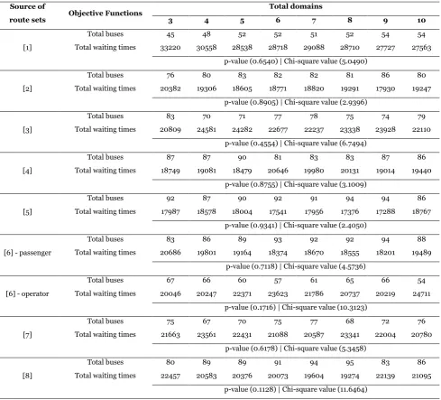
Based on Table 1, the source of route sets are stated in the first column. The second column indicate the objective functions studied. Columns 3–10 record the values of respective measurements in column 2 such that the values in last column is obtained from Uvaraja and Lee (2019). For all the routes of size 4, the solutions from the total domains of 3–9 are comparable with the domain of 10. The number of buses increases as the total waiting times decreases and vice-verse. The results of Uvaraja and Lee (2019) dominate the solutions
from the total domains of 9 for Mandl (1980) and of 4 and 8 for Chakroborty (2003). The total waiting times from the current experiment are higher although the total buses are greater or equal as compared to the previous results. On the other hand, the hypothesis test revealed that the number of domains does not affect the level of solutions for 4 routes as all the p-values are higher than 0.05 and the chi-square values are lower than 14 according to the distribution table.
Table 1. Comparison of results between numbers of domains for 4 routes
Source of
route sets Objective Functions
Total domains
3 4 5 6 7 8 9 10
[1]
Total buses 45 48 52 52 51 52 54 54
Total waiting times 33220 30558 28538 28718 29088 28710 27727 27563
p-value (0.6540) | Chi-square value (5.0490)
[2]
Total buses 76 80 83 82 82 81 86 80
Total waiting times 20382 19306 18605 18771 18820 19291 17930 19247
p-value (0.8905) | Chi-square value (2.9396)
[3]
Total buses 83 70 71 77 78 75 74 79
Total waiting times 20809 24581 24282 22677 22237 23338 23928 22110
p-value (0.4554) | Chi-square value (6.7494)
[4]
Total buses 87 87 90 81 83 83 87 86
Total waiting times 18749 19081 18479 20646 19980 20131 19014 19440
p-value (0.8755) | Chi-square value (3.1009)
[5]
Total buses 92 87 90 92 91 94 94 86
Total waiting times 17987 18578 18004 17541 17956 17376 17288 18767
p-value (0.9341) | Chi-square value (2.4050)
[6] - passenger
Total buses 83 86 89 93 92 92 94 88
Total waiting times 20686 19801 19164 18374 18670 18555 18201 19489
p-value (0.7118) | Chi-square value (4.5736)
[6] - operator
Total buses 67 66 60 57 61 65 66 54
Total waiting times 20046 20247 22371 23623 21786 20737 20219 24711
p-value (0.1716) | Chi-square value (10.3123)
[7]
Total buses 75 67 70 75 77 68 72 76
Total waiting times 21663 23561 22431 21088 20587 23341 22004 20780
p-value (0.6178) | Chi-square value (5.3458)
[8]
Total buses 80 89 89 91 94 95 83 86
Total waiting times 22457 20583 20376 20073 19604 19274 22139 21095
p-value (0.1128) | Chi-square value (11.6464)
Note:
[6]:Nikolić and Teodorović (2014); [7]:Arbex and da Cunha (2015); [8]:Buba and Lee (2018); [9]:Baaj and Mahmassani (1991); [10]:Shih and Mahmassani (1994); [11]:Bagloee and Ceder (2011)
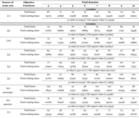
For 5 routes (see, Table 2), the solutions from every total domains are equivalent to each other except for the total domains of 7 and 9 where the total waiting times is reduced for the former solutions with equal number of buses. When compared with the solutions from Uvaraja and Lee (2019), the number of buses are greater with lesser total waiting times. The values of objective functions are significantly different in between the values of total domains which reflects its dependency. On the other hand, the number of domains does not affect the performance of MTS algorithm for some of the route sets of size 6 without including the route sets from Arbex and da Cunha (2015), Chew et al. (2013), Nikolić and Teodorović (2013) and Buba and Lee (2018). For these route
sets, there are at least one parameter value that considerably different from the usual pattern. For examples, 77 buses (total domain of 3) from Chew et al. (2013), 80 buses (total domain of 5) from Nikolić and Teodorović (2013), 77 buses (total domain of 8) from Arbex and da Cunha (2015) and 75 buses (total domain of 3) from Buba and Lee (2018) are highly differ with the respective solutions from the total domain of 10. The statistical test also show that the number of domains affects the quality of solutions. Other route sets produce comparable solutions that are close to each other that prevent their dependency to the number of domains.
Table 2. Comparison of results between numbers of domains for 5 and 6 routes
Source of route sets
Objective Functions
Total domains
3 4 5 6 7 8 9 10
5 routes
[7]
Total buses 87 71 79 73 74 69 74 64
Total waiting times 19275 22856 21468 22696 22472 24326 22518 26262
p-value (0.01550) | Chi-square value (17.3039) 6 routes
[9]
Total buses 74 80 76 79 79 81 83 76
Total waiting times 20181 18680 19647 18883 18713 18328 17911 19558
p-value (0.8590) | Chi-square value (3.2690)
[10] Total buses 72 74 78 81 80 79 83 82
Total waiting times 22547 21342 20883 20097 20281 20527 19686 19869
p-value (0.7010) | Chi-square value (4.6631)
[3]
Total buses 83 97 85 93 99 87 97 88
Total waiting times 19869 16641 19361 17515 16201 18582 16709 18433
p-value (0.0728) | Chi-square value (12.9706)
[4]
Total buses 77 99 109 94 100 106 101 101
Total waiting times 22902 17603 15789 18305 17142 16291 17028 17457
p-value (1.39 x 10⁻⁴) | Chi-square value (29.1021)
[5]
Total buses 90 97 80 92 82 89 100 100
Total waiting times 20761 18485 22597 19147 21726 20200 18040 18147
p-value (0.0129) | Chi-square value (17.7984)
[6] - passenger
Total buses 103 84 91 98 101 102 94 98
Total waiting times 18941 22898 21501 19850 19325 19001 20545 19697
p-value (0.1153) | Chi-square value (11.5248)
[6] - operator
Total buses 76 60 62 68 69 63 66 61
Total waiting times 20780 26518 25595 23199 23164 25020 24198 25946
p-value (0.0931) | Chi-square value (12.2334)
[7] Total buses 65 58 71 64 71 77 73 63
p-value (0.0384) | Chi-square value (14.8200)
[8]
Total buses 75 92 80 91 93 81 92 85
Total waiting times 26554 21437 24580 21536 21157 24768 21310 23091
p-value (0.0099) | Chi-square value (18.5115)
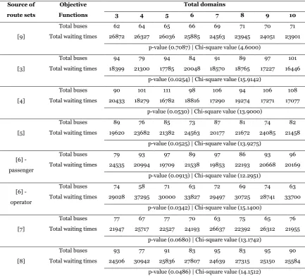
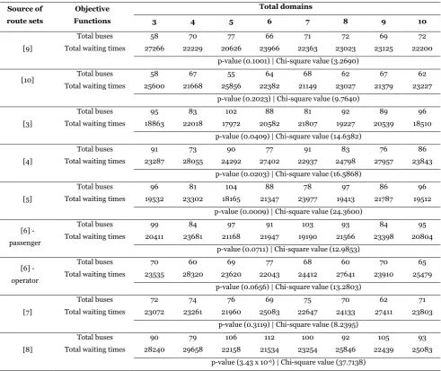
For 7 routes (see, Table 3), 5 out of 8 route sets able to maintain their independency towards the total domain. The route sets of Buba and Lee (2018), Mumford (2013) and Nikolić and Teodorović (2014) show their reliance on total domains based on the lower p-values and higher chi-square values. Likewise, for 8 routes (see, Table 4), the results for Chew et al. (2013), Nikolić and Teodorović (2013), Buba and Lee (2018) and Mumford (2013) depend on the number of domain used. Overall, the quality of solutions from every parameter values
from 3 to 9 are quite similar to the solution from total domains of 10. Some of the solutions from this study are dominated by the solution published in Uvaraja and Lee (2019), by producing higher total waiting times with the same number of buses. Apart from that, the objective functions values for the route sets ofShih and Mahmassani (1994) from the total domain of 8 is better than the output from the total domain of 10 with lesser waiting times.
Table 3. Comparison of results between numbers of domains for 7 routes
Source of route sets
Objective Functions
Total domains
3 4 5 6 7 8 9 10
[9]
Total buses 62 64 65 66 69 71 70 71
Total waiting times 26872 26327 26036 25885 24563 23945 24051 23901
p-value (0.7087) | Chi-square value (4.6000)
[3]
Total buses 94 79 94 84 91 89 97 101
Total waiting times 18399 21300 17785 20048 18570 18765 17227 16446
p-value (0.0254) | Chi-square value (15.9142)
[4]
Total buses 90 101 111 98 106 94 106 108
Total waiting times 20433 18279 16782 18816 17290 19274 17271 17077
p-value (0.0530) | Chi-square value (13.9000)
[5]
Total buses 89 76 85 73 87 81 74 82
Total waiting times 19620 23682 21382 24563 20177 21672 24085 21458
p-value (0.0525) | Chi-square value (13.9275)
[6] - passenger
Total buses 79 93 97 89 97 86 93 96
Total waiting times 24535 20994 19709 21538 19853 22193 20668 20169
p-value (0.0913) | Chi-square value (12.2951)
[6] - operator
Total buses 74 58 71 63 72 69 74 63
Total waiting times 29028 37295 30000 33827 29497 30725 28741 33700
p-value (0.0342) | Chi-square value (15.1400)
[7]
Total buses 77 67 77 70 63 75 65 76
Total waiting times 21947 25717 22527 24193 26637 22392 26312 21955
p-value (0.0680) | Chi-square value (13.1742)
[8]
Total buses 93 77 91 83 95 83 95 90
Total waiting times 24506 30942 25836 27807 24639 27315 25150 25584
p-value (0.0486) | Chi-square value (14.1512)
For the route sizes from 9–12 as shown in Tables 5 and 6, solutions from all the route sets are highly dependent on the total domains. This is because the solutions between the total
number of buses while decreasing the total waiting times. Generally, the dependency of the solution towards number of domains increases as the route size becomes larger. It can be seen clearly that most of the solutions are analogous to each other. The objective functions values are always conflicting
such that the increase in number of buses attributes to the reduction in total waiting times and vice versa. This experiment proves that the result produced by Uvaraja and Lee (2019) that total domain of 10 yield acceptable solutions for all the route sets.
Table 4. Comparison of results between numbers of domains for 8 routes
Source of route sets
Objective Functions
Total domains
3 4 5 6 7 8 9 10
[9]
Total buses 58 70 77 66 71 72 69 72
Total waiting times 27266 22229 20626 23966 22363 23023 23125 22200
p-value (0.1001) | Chi-square value (3.2690)
[10] Total buses 58 67 55 64 68 62 67 62
Total waiting times 25600 21668 25856 22382 21149 23027 21379 23227
p-value (0.2023) | Chi-square value (9.7640)
[3]
Total buses 95 83 102 88 81 92 89 96
Total waiting times 18863 22018 17972 20582 21807 19227 20539 18510
p-value (0.0409) | Chi-square value (14.6382)
[4]
Total buses 91 73 90 77 91 83 76 86
Total waiting times 23287 28055 24292 27402 22937 24798 27957 23843
p-value (0.0203) | Chi-square value (16.5868)
[5]
Total buses 96 81 104 88 78 97 86 96
Total waiting times 19532 23302 18165 21347 23977 19413 21787 19512
p-value (0.0009) | Chi-square value (24.3600)
[6] - passenger
Total buses 99 84 97 91 103 93 84 95
Total waiting times 20411 23681 21168 21947 19190 21566 23398 20804
p-value (0.0711) | Chi-square value (12.9853)
[6] - operator
Total buses 70 60 69 77 68 60 70 65
Total waiting times 23535 28320 23620 22043 24412 27641 23910 25479
p-value (0.0656) | Chi-square value (13.2803)
[7]
Total buses 72 74 76 69 75 70 62 71
Total waiting times 23072 23261 21960 25083 22647 24133 27411 23803
p-value (0.3119) | Chi-square value (8.2395)
[8]
Total buses 90 79 106 112 100 92 105 93
Total waiting times 28240 29658 22158 21534 23254 25846 22439 25083
p-value (3.43 x 10⁻⁶) | Chi-square value (37.7138)
Table 5. Comparison of results between numbers of domains for 9, 10, and 11 routes
Source of route sets
Objective Functions
Total domains
3 4 5 6 7 8 9 10
[7]
9 routes
Total buses 72 62 71 70 59 70 61 58
Total waiting times 27738 31618 27166 28671 34001 28914 32775 34381
p-value (0.0312) | Chi-square value (15.4026) 10 routes
Total buses 106 80 70 94 80 74 87 81
Total waiting times 18293 24373 28055 20285 24090 26009 22066 23903
11 routes
Total buses 95 72 96 78 72 60 62 67
Total waiting times 19509 25221 18885 23673 25257 30237 30009 26863
p-value (2.69 x 10⁻¹³) | Chi-square value (73.6541)
Table 6. Comparison of results between numbers of domains for 12 routes
Source of route sets
Objective Functions
Total domains
3 4 5 6 7 8 9 10
[11]
Total buses 91 80 66 83 77 83 78 73
Total waiting times 19511 20780 25625 20031 21649 20203 21259 22520
p-value (0.0162) | Chi-square value (17.1845)
[6] - passenger
Total buses 97 79 97 86 77 95 88 95
Total waiting times 20910 29941 25181 27303 29892 24734 27178 24675
p-value (6.15 x 10⁻³) | Chi-square value (25.5122)
[6] - operator
Total buses 89 70 58 80 67 62 61 52
Total waiting times 20949 26274 29243 22746 27905 28916 29665 33828
p-value (1.17 x 10⁻⁹) | Chi-square value (55.5247)
[7]
Total buses 48 95 71 62 84 74 68 62
Total waiting times 43269 20854 27891 32334 23020 26169 29226 31162
p-value (4.21 x 10⁻¹⁷) | Chi-square value (92.2755)
[8]
Total buses 138 108 88 71 73 87 81 72
Total waiting times 21453 28214 35844 42043 32989 37630 38458 42468
p-value (7.57 x 10-37) | Chi-square value (186.6765)
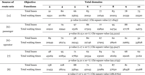
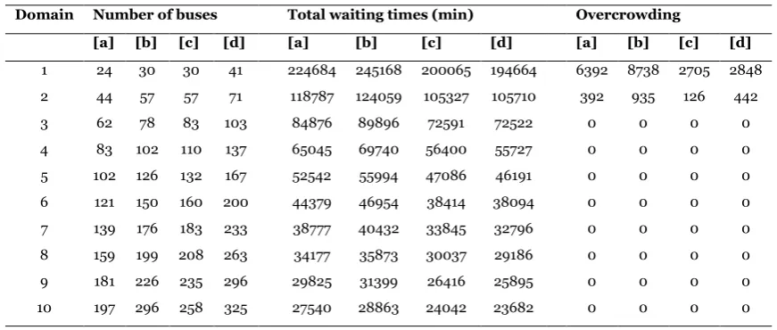
B. Results of Extended Model
In Uvaraja and Lee (2019), the route set of size 4 from Buba and Lee (2018) are experimented. In this study, the investigation is continued for 6–12 routes using the extended model. The algorithm is run for 10 times and the average solution for every domain are tabulated. As there is no previous solution in the literature, comparison is not possible for all the routes.
Based on the Table 7, the number of buses increase and the total waiting times decrease as the domains become higher. This is due to the range of frequency allocated for every domain also increases from 27 to 369 for the time period of 18 hours. Moreover, the first two domains show overcrowding which caused by inadequate number of buses to fetch all the passengers at a timeslot of the routes. The number of buses and total waiting times are greater as compared to the solutions in Tables 1– 6 although same data sets and setting for the MTS algorithm are employed. For instance, the number of buses and total waiting times for the
standard model without timeslot are 85 buses and 23091 munites respectively for 6 routes from Buba and Lee (2018) as shown in Table 2. According to Table 7, the objective values
from domain 6 for 6 routes are 121 buses and 44379 minutes of waiting times. The increase in total buses and waiting times are caused by the addition of layover time and dwell time into the bus route trip and the difference in frequency for various timeslots that changes the time interval between consecutive buses. Overall, the number of buses increase when the size of route sets also escalate. The total waiting times and
overcrowding are not directly influenced by the increase in number of routes as they are calculated based on the routes frequency which is in the same range for each domain regardless of the number of routes.
passenger’s point of view is measured, the solution with lower
total waiting times is chosen.
V. CONCLUSIONS
In this paper, we conducted an analysis with varies parameter values to evaluate the efficiency of MTS algorithm for urban transit frequency optimization problem. A statistical test is employed to check the dependency of the number of domains on the solution quality. Besides, in order to extend the computational study of frequency optimization problem, MTS algorithm is tested with larger route sets from Mumford (2013). The results of this study leads to the following remarks: (1) the values of total buses and waiting times are
subject to the number of domains and its dependency increases as the route size becomes higher; (2) larger number of domains must be assigned to obtain better solutions that reduce both of the objective values and therefore the number of domains of 10 is most preferred as it is able to produce better solutions for most of the route sets than other number of domains; (3) feasible solutions are obtained for higher number of route sets with sizes 6, 7, 8, and 12 that indicates the effectiveness of MTS algorithm. Based on the experiments, the performance of MTS algorithm for frequency optimization problem is highly influenced by the number of domains although it gives comparable solutions as compared to other methods.
Table 7. Results obtained for extended model
Domain Number of buses Total waiting times (min) Overcrowding
[a] [b] [c] [d] [a] [b] [c] [d] [a] [b] [c] [d]
1 24 30 30 41 224684 245168 200065 194664 6392 8738 2705 2848
2 44 57 57 71 118787 124059 105327 105710 392 935 126 442
3 62 78 83 103 84876 89896 72591 72522 0 0 0 0
4 83 102 110 137 65045 69740 56400 55727 0 0 0 0
5 102 126 132 167 52542 55994 47086 46191 0 0 0 0
6 121 150 160 200 44379 46954 38414 38094 0 0 0 0
7 139 176 183 233 38777 40432 33845 32796 0 0 0 0
8 159 199 208 263 34177 35873 30037 29186 0 0 0 0
9 181 226 235 296 29825 31399 26416 25895 0 0 0 0
10 197 296 258 325 27540 28863 24042 23682 0 0 0 0
Note: [a]: 6 routes; [b]: 7 routes; [c]: 8 routes; [d]: 12 routes
VI. ACKNOWLEDGMENT
This research was supported by Fundamental Research Grant Scheme (FRGS) 01-01-16-1867FR (Ministry of Higher Education, Malaysia). The authors would like to thank reviewers for their time to thoroughly review and provide constructive comments for improvements of the manuscript.
VII.REFERENCES
Afandizadeh, S, Hassan, K & Narges, K 2013, ‘Bus fleet optimization using genetic algorithm a case study of Mashhad’,International Journal of Civil Engineering, vol. 11, no. 1, pp. 43–52.
159 pp. 355–376.
Baaj, MH & Mahmassani, HS 1991, ‘An AI-based approach for transit route system planning and design’, Journal of Advanced Transportation,vol.25, no. 2, pp. 187–209. Bagloee, SA & Ceder, AA 2011, ‘Transit-network design
methodology for actual-size road networks’,Transportation Research Part B: Methodological, vol. 45, no. 10, pp. 1787– 804.
Buba, AT & Lee, LS 2018, ‘A differential evolution for simultaneous transit network design and frequency setting problem’,Expert Systems With Applications, vol. 106, pp. 277–89.
Chakroborty, P 2003, ‘Genetic algorithms for optimal urban transit network design’, Computer-Aided Civil and Infrastructure Engineering, vol. 18, no. 3, pp. 184–200. Chew, JSC, Lee, LS & Seow, HV 2013, ‘Genetic algorithm for
biobjective urban transit routing problem’, Journal of Applied Mathematics, Article. ID 698645, 15 pages.
Crainic, TG, Gendreau, M & Farvolden, JM 2000, ‘A simplex-based tabu search method for capacitated network design’,INFORMS Journal on Computing, vol. 12, no. 3, pp. 223-236.
Gendreau, M, Laporte, G, Musaraganyi, C & Taillard, ÉD 1999, ‘A tabu search heuristic for the heterogeneous fleet vehicle routing problem’,Computers & Operations Research, vol. 26, no. 12, pp. 1153-1173.
Mandl, C 1980, ‘Evaluation and optimization of urban public transportation networks’,European Journal of Operational Research, vol. 5, no. 6, pp. 396–404.
Mumford, CL 2013, ‘New heuristic and evolutionary operators for the multi-objective urban transit routing problem’, In IEEE Congress of Evolutionary Computation, pp. 939–46. Nikolić, M & Teodorović, D 2013, ‘Transit network design by
bee colony optimization’,Expert Systems With Applications, vol.40, pp. 5945–55.
Nikolić, M & Teodorović, D 2014, ‘A simultaneous transit network design and frequency setting: Computing with bees’, Expert Systems With Applications, vol.41, no. 16, pp. 7200– 09.
Shih, MC & Mahmassani, HS 1994, ‘A design methodology for bus transit networks with coordinated operations’,Technical Report.
Uvaraja, V & Lee, LS 2019, ‘Multiple tabu search for multiobjective urban transit scheduling problem’, ASM Science Journal, vol. 12, special issue 1, pp. 150–173. Xu, J & Kelly, JP 1996, ‘A network flow-based tabu search
heuristic for the vehicle routing problem’, Transportation
Science, vol. 30, no. 4, pp. 379-393.
Xu, J, Chiu, SY & Glover, F 1998, ‘Fine‐tuning a tabu search algorithm with statistical tests’,International Transactions in Operations Research, vol. 5, no. 3, pp. 233–44.