Error control co d in g for co n stra in ed ch a n n els
A thesis subm itted for the degree of Doctor of Philosophy
in Electronic and Electrical Engineering
June 1999
Chris M atrakidis
UCL
ProQuest Number: 10011209
All rights reserved
INFORMATION TO ALL USERS
The quality of this reproduction is dependent upon the quality of the copy submitted.
In the unlikely event that the author did not send a complete manuscript and there are missing pages, these will be noted. Also, if material had to be removed,
a note will indicate the deletion.
uest.
ProQuest 10011209
Published by ProQuest LLC(2016). Copyright of the Dissertation is held by the Author.
All rights reserved.
This work is protected against unauthorized copying under Title 17, United States Code. Microform Edition © ProQuest LLC.
ProQuest LLC
789 East Eisenhower Parkway P.O. Box 1346
A cknow ledgem ents
I wish to express my thanks to my supervisor, Professor John J. O ’Reilly for his advice and guidance throughout the course of this study.
A b stract
Channel coding is an im portant consideration influencing the design of a com m unications system. In particular, error control coding is used to detect an d /o r correct errors and line coding to modify the characteristics of the tran sm itted signal to suit other constraints of the channel, such as restricted frequency re sponse.
This thesis explores aspects of channel coding for such constrained channels w ith emphasis given to error control coding.
Specifically, the first chapter of this thesis presents a general overview of channel coding, presents the organisation of the thesis and details the main contribu tions.
T he second chapter gives an overview of the principles of error control cod ing and line coding and explains a few term s th a t are commonly used in the rem ainder of the thesis.
One kind of constrained channel investigated here is the binary asymm etric error channel, where error transitions from one to zero occur w ith different probability th an from zero to one. Error correcting codes for this channel and their properties are investigated in the th ird chapter.
Run length lim ited channels are the subject of the fifth chapter. A new cod ing structure is proposed th a t offers advantages in performance over the one conventionally used for error control in such channels.
The sixth chapter introduces peak power constraints present in m ulti-carrier systems. Codes th a t can be used limit the peak to average power ratio of such systems are presented and the application of the coding structure of the fifth chapter is also discussed.
Table o f contents
Acknowledgements ... 2
A bstract ... 3
Table of contents ... 5
List of figures ... 10
List of tables ... 13
1 Introduction ... 15
1.1 Organisation of this thesis ... 16
1.2 Outline of main contributions ... 17
1.3 Sum m ary ... 20
2 Aspects of channel coding ... 21
2.1 Introduction ... 21
2.2 Brief description of common coding term s ... 21
2.2.1 Code rate ... 21
2.2.2 Hamming distance ... 22
2.2.3 E rror correcting/detecting capability ... 22
2.3 Line coding ... 23
2.3.1 D isparity control line c o d in g ... 23
2.3.2 R un length limiting line coding ... 24
2.4 E rror control c o d in g ... 24
2.5 Sum m ary ... 26
3 Asymmetric error control c o d e s ... 27
3.1 Introduction ... 27
3.2 Asymmetric errors ... 27
3.3 Asymmetric distance ... 29
3.4 Error correcting capabilities of a code C ... 30
3.5 Relation between the asymmetric Z-channel error correcting and sym metric error correcting ca p a b ilitie s... 33
3.5 Code word properties ... 34
3.5.1 New properties ... 35
3.5.2 Code size ... 38
3.6 Integer programming upper b o u n d ...39
3.7 Lower bound on the number of code-words ... 41
4 Combined disparity and error control coding ... 44
4.1 Introduction ... 44
4.2 Line coding ... 44
4.2.1 Disparity limited line c o d e s ... 45
4.3 A lternate dictionary line codes ... 46
4.4 E rror correcting line c o d e s ... 49
4.4.1 Proposed technique... 50
4.4.2 Exam ple... 52
4.5 Asymmetric error correcting codes ... 53
4.5.1 A lternative encoding scheme... 59
4.6 Summary ... 60
5 Combined run-length limited and error control coding ... 62
5.1 Introduction ... 62
5.2 Overview ... 63
5.3 Proposed line code ... 64
5.3.1 Im plem entation details ... 67
5.4 Implementing a line code ... 70
5.3.3 E rror extension ... 75
5.4 Examples of designed codes ... 76
5.5 Summary ... 77
6 Peak power constrained coding for m ulti-carrier systems ... 80
6.1 Introduction ... 80
6.2 M ulti-carrier m o d u la tio n ... 81
6.3 Peak to average power ratio ... 83
6.4 Encoder structure ... 86
6.5 Binary phase shift keying (BPSK) ... 87
6.5.1 Search algorithms ... 91
6.5.2 R e s u lts ... 92
6.6 Q uadrature phase shift keying (QPSK) ... 95
6.7 Consideration of systems w ith a large number of c a r r ie r s ... 101
6.8 Aspects of error control ... 101
6.9 Summary ... 102
7 Concluding remarks ... 104
7.1 Introduction ... 104
7.3 Suggestions for further w o r k ... 106
A Limits of constant weight codes ... 108
A .l Introduction ... 108
A .2 Trivial values ... 108
A .3 Johnson’s bounds ... 109
A .4 Bounds using linear programming ... 110
A .4.1 D elsarte’s bound ... 110
A .4.2 Van P u l’s bound ... I l l A .4.3 Additional constraints ... 117
A .5 Tables of upper and lower bounds of A(n, d,w ) ... 117
A .5 Summary ... 118
List o f figures
1.1 Subdivisions of c o d in g ... 15
2.1 Family tree of error correcting codes ... 25
3.1 A general binary communication channel ... 27
3.2 Z channel ... 28
3.3 Illustrating the quantity A (x , u) and the asymmetric distance of two binary vectors ... 29
3.4 T he Hamming distance of two binary vectors ... 30
3.5 An error p ath between two code-words w ith d// = 3 in a symmetric error channel ... 31
3.6 An error between the same co de-words as in Fig. 3.5 in the Z-channel 32 3.7 A code w ith n = f |A ] ... 37
3.8 A code w ith n = 3A, when A is even ... 38
4.1 Some co de-words and their disparity ... 46
4.2 Frequency response of the 3B4B line code of table 4 . 2 ... 48
4.3 A cascaded error control and line coding system ... ... 49
4.4 The 3 bit code-word space ... 51
4.6 Frequency response of the new 9-b it error correcting line code .... 54
4.7 Power spectral density of the new 11-bit asymmetric Z-channel error correcting line code ... 56
4.8 Power spectral density of the reduced 11-bit asymmetric Z-channel error correcting line code ... 58
4.9 Power spectral density of the same 11-bit code using the more...com plicated e n c o d e r ... 59
5.1 Conventional cascaded coding arrangem ent ... 62
5.2 Bliss’ coding sc h e m e ...64
5.3 E rror correcting line code encoding and decoding arrangem ent .... 64
5.4 Proposed coding arrangement ... 65
5.5 Shuffling of the bits to satisfy run-length bounds ... 65
5.6 Exam ple of bit insertion in a code-word ... 66
5.7 N um ber of configurable logic blocks for different values of the cost f u n c tio n ... 72
5.8 Num ber of configurable logic blocks for different values of th e modified cost function ... 75
5.9 Num ber of CLBs for different code-word le n g th s ... 78
6.1 Envelope power of a four sub-carrier signal ... 84
6.3 PA PR reduction possible with Jones’ scheme ... 88
6.4 Uncoded and system atic bits as a function of the PA PR gain for a 4 sub-carrier system ... 93
6.5 Uncoded and system atic bits as a function of the PA PR gain for an 8 sub-carrier system ... 93
6.6 Uncoded and system atic bits as a function of the PA PR gain for a 12 sub-carrier system ... 94
6.7 Uncoded and system atic bits as a function of the PA PR gain for a 16 sub-carrier system ... 94
6.8 Uncoded and system atic bits as a function of the PA PR gain for a 4 sub-carrier QPSK system ... 97
6.9 Uncoded and system atic bits as a function of the PA PR gain for a 6 sub-carrier QPSK system ... 98
6.10 Uncoded and system atic bits as a function of the PA PR gain for an 8 sub-carrier QPSK system ... 98
6.11 Possible PA PR gain for one redundant carrier ( Q P S K ) ... 100
6.12 Peak power reduction w ith added redundant carrier (QPSK) ... 100
List
o ftables
3.1 Bounds on the asymmetric Z-channel error correcting code size ... 40
4.1 A 3B4B alternate line code w ith the last bit indicating inversion of the code-word ... 47
4.2 A 3B4B alternate line code employing zero disparity words in b o th dictionaries ... 48
4.3 An error correcting alternate line code w ith 9 bits and minimum dis tance 3 ... 53
4.4 New 11-b it single asymmetric Z-channel error correcting line code w ith 95 code-word pairs ... 57
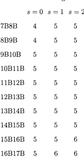
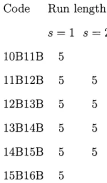
5.1 M aximum run-length of various codes, s is the number of uncon strained bit positions ... 68
5.2 Codes of table 5.1 presenting an improvement in run-length. s is the number of unconstrained bit positions ... 69
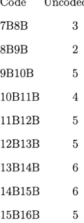
5.3 Maximum number of uncoded bits th a t can be present in line code .. 74
5.4 Uncoded bits for various codes including the unconstrained one ... 77
6.1 Num ber of encoded bits required for Jones’ scheme ... 89
6.2 P A PR gain possible by using simple code compared w ith best possible gain using comparable scheme ... 90
6.4 PA PR gain possible by using simple code compared to the best pos
sible gain using comparable code (QPSK) ... 96
6.5 Encoder and decoder arrangement for 2dB g a i n ... 99
A .l A (n ,4 ,rc).. ... 112
A .2 A { n ,6 ,w ).. ... 113
A .3 A (n ,8 ,u ;).. ... 114
A .4 A{n, 10, rc) ... 115
A .5 A{n, 12, w) ... 116
1 In trod u ction
This thesis addresses a number of points relevant to coding for communica tions transm ission and storage. In general, coding is the mapping of one d ata sequence into another in such a way th a t a desired property is achieved.
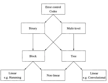
Figure 1.1 shows the main categories th a t coding theory deals with. These are cryptography, where the source data are modified to improve security, channel coding where redundancy is added in order to improve reliability and source coding th a t attem p ts to remove any redundancy present in the source data. This thesis deals with channel coding, which is also shown as subdivided into error control and line coding.
Coding
Channel
coding
Line
coding
Cryptography Source
coding
Error control
coding
Figure 1.1: Subdivisions of coding
transm ission. In contrast, error control coding is used to correct a n d /o r detect transm ission errors after they have occurred.
The m otivation for this work was th a t the techniques normally designed for generalised channels are not applicable to certain constrained channels. In general, we may wish to m atch the signal to th e channel in more subtle ways th a n normal, or to incorporate more th an one coding objective in a single code. An example of the former is coding to control errors which affect asymm etrically “I ’s” and “O’s” (asymmetric channel). An example of the la tte r is when a channel requires both line and error control coding: the use of cascaded codes has some disadvantages compared w ith a single code designed to m eet b o th requirements.
1.1 O rg a n isa tio n o f th is th e sis
Following this introduction, the next chapter provides a brief description of the basic principles of channel coding. Several commonly used term s are explained and some commonly used terms are introduced. Continuing this chapter, line and error control codes are discussed in more detail, and their various subdivi sions are described.
The fourth chapter deals w ith coding for channels where bo th disparity control (see section 2.3.1) and error control are desirable. A new error correcting line code structure is proposed th a t can be applied to codes designed for the binary sym m etric and asymmetric channels.
The fifth chapter deals w ith coding for channels where run length lim iting com bined w ith error protection is required. High rate codes th a t can be combined w ith system atic error control codes are discussed th a t exhibit negligible reduc tion of the error correcting capability of the error control code. Furtherm ore, a technique to design line codes is proposed th a t optimises the source word to channel word mapping to allow efficient implem entation of the code.
The sixth chapter discusses coding techniques th a t can be applied in systems where multiple carriers are utilised simultaneously. The m ain aim here is to reduce the peak to average power ratio of such systems, w ith a small increase in redundancy and a low level of im plem entation complexity.
Finally, the seventh chapter concludes the thesis and provides some suggestions for future work.
1.2 O u tlin e o f m ain co n trib u tio n s
The m ain contributions of this thesis are the following:
• Identification of previously unknown asymmetric error correcting code prop erties.
• E laboration of a new disparity error correcting line coding structure.
• D em onstration for the first tim e of asymmetric error correcting line codes for disparity control.
• Presentation of a coding structure th a t can achieve overall high coding rate in combined run length limited codes together w ith conventional system atic error correcting codes, without a noticeable increase in error rate.
• Development of optim isation techniques th a t provide a reduction in th e hard ware complexity of line codes.
• Study of the trade-off between im plementation complexity and performance in high rate peak to average power ratio reducing codes for m ulti-carrier systems.
The following papers have been published or have been accepted for publication during the course of this study.
[1] S. Fragiacomo, C. M atrakidis, and J. J. O ’Reilly, “A new error correct ing line code,” in IT S /IE E E ROC&C International Telecommunications Symposium, (Acapulco, Mexico), pp. 54-58, Oct. 1996.
[2] S. Fragiacomo, C. M atrakidis, and J. J. O ’Reilly, “Exploiting soft decision decoding for error correcting line codes,” in IE E E IC C S /IS P A C S Confer ence Proceedings, vol. 2, (Singapore), pp. 638-642, Nov. 1996.
[3] S. Fragiacomo, C. M atrakidis, and J. J. O ’Reilly, “Soft decision error cor recting line code for optical data storage,” in LEO S Conference Proceed
[4] S. Fragiacomo, Y. Bian, A. Popplewell, C. M atrakidis, and J. J. O ’Reilly, “An accelerated simulation technique for evaluating communication sys tems using EEC,” in Proceedings of the European Conference on Networks and Optical Communications, vol. 2, (Antwerp, Belgium), pp. 145-148, June 1997.
[5] C. M atrakidis and J. J. O ’Reilly, “A block decodable line code for high speed optical communication,” in IE E E International Symposium on Inform ation
Theory, (Ulm, Germany), p. 221, June 1997.
[6] S. Fragiacomo, C. M atrakidis, and J. J. O ’Reilly, “A class of low complex ity line codes,” in IE E E International Symposium on Inform ation Theory,
(Ulm, Germany), p. 219, June 1997.
[7] S. Fragiacomo, G. M atrakidis, and J. J. O ’Reilly, “Class of low complexity line codes for optical data storage and communications,” in The Pacific R im Conference on Lasers and Electro-Optics, (Ghiba, Japan), pp. 92-93, July 1997.
[8] C. M atrakidis and J. J. O’Reilly, “Limiting the maximum ru n -len g th of block turbo codes,” in Proceedings of the International Symposium on
Turbo Codes & Related Topics, (Brest, France), pp. 220-222, Sept. 1997.
[10] s. Fragiacomo, C. M atrakidis, and J. J. O ’Reilly, “M ulticarrier transm is sion peak-to-average power reduction using simple block code,” Electronics Letters^ vol. 34, pp. 953-954, May 1998.
[11] S. Fragiacomo, C. M atrakidis, A. Popplewell, and J. J. O ’Reilly, “Novel accelerated technique for low bit error rate communication system s,” lE E Proceedings on Communications, vol. 145, pp. 337-341, Oct. 1998.
1.3 S u m m a ry
2 A sp ects o f channel coding
2.1 In tr o d u c tio n
Channel coding is the process whereby the reliability of a channel is improved by adding redundancy into the transm itted data. Channel coding is usually subdivided into two categories, line coding and error control coding, th a t use this redundancy in different ways. Line coding modifies some properties of the tran sm itted sequence trying to improve the reliability of the transm ission, while error control coding attem pts to correct a n d /o r detect errors at th e receiver.
The m ain aim of this chapter is to provide a brief introduction to those two channel coding categories. We begin by outlining in section 2.2 the common term s th a t are going to be used in the rem ainder of the thesis. In section 2.3 we tu rn our attention to briefly describing the background and key ideas of line coding. Section 2.4 consists of an overview of the principles of error control coding. Finally, the chapter concludes w ith a short summary.
2.2 B r ie f d escrip tio n o f com m on co d in g term s
There are several common terms relating to channel coding th a t are used throughout this thesis. The more im portant ones are as follows.
2.2.1 Code rate
the number of encoded symbols th a t represent the same information. If several coding stages are cascaded, then the overall rate is the product of the rates of all stages.
2.2.2 Hamming distance
The Hamming distance between two sequences is the number of symbol posi tions in which the two sequences differ. Also of im portance is the minimum Hamming distance of a code, which is the minimum Hamming distance calcu lated between all possible pairs of co de-words in the code.
2.2.3 E rror correcting/detecting capability
The error correcting/detecting capability of a code is the maxim um num ber of single symbol or bit errors th a t are guaranteed to be corrected/ detected by the code. However, depending on the actual code used and the decoder im plem entation, there may be specific patterns of more errors th a t can be cor rec te d / detected.
2.2.4 E rror extension
2.2.5 System atic codes
W hen the information symbols th a t are to be tran sm itted are present unm odi fied in the encoded sequence then the code is a system atic one, otherwise it is called non-system atic. The symbols of a code-word of a system atic code can be divided into information symbols and redundancy symbols. Many commonly used error correcting codes are systematic, while most line codes are not.
2.3 L ine co d in g
Lines codes are codes designed to modify the characteristics of the tran sm itted d a ta in a way th a t suits the transmission channel. This improves the reliability of th e transmission. The prim ary common requirements of a line code are[12]:
• to minimise vulnerability to inter-sym bol interference (ISI) and noise;
• to enable extraction of a timing reference; and
• to achieve the first two ends w ith only modest redundancy.
T he two most common categories of line coding are disparity control and run length limiting.
2.3.1 Disparity control line coding
tra n sm itter and the receiver and facilitates transmission through channels w ith poor signal to noise ratio at low frequencies [13].
A disparity control line code utilises the added redundancy to limit the disparity of the tran sm itted sequence between bounds at any point in the sequence. This is usually achieved by bounding the value of the disparity at th e end of each code-word.
2.3.2 R un length limiting line coding
A run is a sequence of consecutive identical symbols; run length is the number of consecutive identical symbols. Run length limiting coding is used when the length of the runs needs to be limited. An upper limit allows the extraction of th e tim ing information from the transm itted sequence by guaranteeing the presence of enough signal transitions. A lower limit in the run length is also used on several systems to reduce the inter-sym bol interference [14].
2.4 Error con trol co d in g
E rror control codes (ECCs) are codes designed to detect or correct errors th a t were inserted during the d a ta sequence transmission. The two m ain categories of ECC are forward error correction (EEC) where some error correction is per formed at the receiver, and autom atic repeat request (ARQ) where the receiver detects the errors and requests the retransm ission of the corrupted informa- tion[15].
Block Binary
Non-linear Error control
Codes
Linear
e.g. Hamming
Linear
e.g. Convolutional Multi-level
Tree
Figure 2.1: Family tree of error correcting codes
split into two other sub-categories, namely block and tree codes. Block codes only depend on the current information word for encoding and decoding, while tree codes utilise memory and the encoding and decoding of each code-word is dependent on a specific number of previous code-words. Furtherm ore, both tree and block codes can be subdivided into linear and nonlinear codes. Convo lutional codes are an im portant category of linear tree codes, while Hamming, BCH and Reed-Solomon are three well known categories of linear block codes. Reed-Solomon codes are multi-level, while the other are usually binary.
The error correcting capability t of a code is usually (i.e. for symm etric errors) dependent on the minimum Hamming distance d between all pairs of code words. For such codes this relationships is given by the formula
Alternatively, the same code can be used to detect up to 2t errors or to correct
2t erasures.
A nother im portant distinction in forward error control systems is to do w ith the way the decoder performs the detection. The simplest decoder architecture only uses the received word hard-lim ited to ones and zeros (in the binary case) and assumes th a t possible errors are equally probable in all the symbols. This kind of decoder is called a hard decision decoder. An alternative is a decoder th a t uses inform ation about the probability of error in all symbols, obtained from the analogue value of the received information. These are called soft decision decoders and can typically correct more (up to 2t) errors th an hard decision ones. However, their im plem entation is more complicated and under extrem e conditions there is the possibility th a t the may correct fewer errors th a n a hard decision decoder.
2.5 S u m m ary
3 A sym m etric error control codes
3.1 In tr o d u c tio n
This chapter begins with a brief description of the asymmetric channel. Some well known properties of asymmetric Z-channel error correcting codes are th en described, followed by a number of properties th a t were discovered during this study of the channel. Those properties are subsequently used to derive upper bounds on the size of codes th a t correct asymmetric Z-channel errors.
3.2 A sy m m e tr ic errors
0 0
1
1-p
Figure 3.1: A general binary communication channel
a 1, then we have a 0-error, and its probability is shown in the figure w ith the symbol q.
In m ost cases, those two probabilities are considered to be independent and equal. In such cases we have w hat is known as the binary symm etric channel.
There are some cases though, where these two probabilities cannot be considered equal. Then, we have an asymmetric error channel.
1
1-p
Figure 3.2; Z channel
One such (extreme) case is the Z-channel, which is shown in figure 3.2. In this case, the probability of a 0-error is zero, b ut the probability of 1-erro r is p. This is the case in some optical communication systems [16] and some d a ta storage systems [17].
3.3 A sy m m e tr ic d ista n ce
An im portant concept for the understanding of Z-channel error-control codes is the asymmetric distance.
0 0 1 1
I\ A V
B
1 0 0 0Figure 3.3: Illustrating the quantity A'(x, u) and the asymmetric distance of two binary vectors: A ( A ,B ) = 1, A (B , A ) = 2 and d^(A , B) = m ax{A (A , B ), A (B , A )} = 2
The asymmetric distance is best defined using the quantity A (x , u) which is defined by A (x , u) = \{i\xi = OAu% = 1}|, where x, u are equal length and w ith symbols = 1 ,2 ,.... This means th a t A (x, u) is the num ber of positions where x is zero and u is one.
Figure 3.3 dem onstrates the one directional nature of A (x , u). In the above example, A (A , B) = 1 and A (B , A) = 2.
Now, the asymmetric distance u) is defined as
dy^(x, u) = m ax{A (x, u), A (u , x)}.
So, in the example shown in figure 3.3, B) = 2.
0 0 1 1
I\ l\
\l M
B
1 0 0 0Figure 3.4: The Hamming distance of two binary vectors d //(A ,B ) = A (A , B) + A (B , A ) = 3
In figure 3.4 we see the same two vectors, only this tim e the arrows are bidi rectional, denoting the symmetric nature of the Hamming distance. In this example, d //(A , B) = 3.
As we can easily see, d ^(x , u) < d/f(x, u) < 2d^(x, u). The exact relation between dA and d n is
2dy^(x, u) = d //(x , u) + |w(x) - tc(u)|,
where tc(x) is the Hamming weight of the binary vector x and is equal to the num ber of “I ’s” in the vector.
3 .4 Error co rrectin g c a p a b ilities o f a co d e C
T he error correcting capabilities of a code C can be described by using two quantities, the minimum asymmetric distance A, and the minimum Ham m ing distance d.
T he minimum Hamming distance is defined by
and the minimum asymmetric distance by
A = m in{d^(x, u) | x, u G C; x u}.
As is the case between the asymmetric and the Hamming distance of two code words, it is fairly easy to show th a t A < d.
Error
!---000
001
o il
111
Figure 3.5: An error path between two code-words with d n = 3 in a symmetric error channel
Code C can correct up to K symmetric errors when 2 K + 1 < d. An example of why this is the case can be seen in figure 3.5. In this example the two code words A = {0, 0,0} and B = {1,1,1} are shown along w ith a possible error p a th between them. The Hamming distance between these words is 3. If during the transm ission through a symmetric error channel, the word {0,0,1} is received, there are two possible cases. Either A was tran sm itted and one error occurred, or B was transm itted and two errors occurred. Assuming the probability of one error occurring is bigger th an the probability of two errors occurring, we have to assume th a t one error occurred. This however means th a t we can’t correct two errors in such a code.
Error
A H
---( B
000
001
o i l
111
Figure 3.6: An error path between the same code-words as in Fig. 3.5 in the Z-channel. Note th a t dA is also 3
is also 3. Now if the word {0,0,1} is received after the transm ission through a z-channel, we know th a t B was transm itted and two errors have occurred. There is no way th a t A was transm itted and one error occurred, due to the one directional nature of the errors in this channel. (Note the arrows in figure 3.6).
We have seen an example, and it can be proved th a t for a given code the maxim um values of T and K have the relationship Tmax > d^max be. a code can correct at least as many asymmetric Z-channel errors as symm etric ones. This is opposite to the relationship between the symmetric and asymmetric distance, A < d.
However, Varshamov[18] has proven th a t most linear codes can correct the same num ber of symmetric and asymmetric Z-channel errors, so in order to gain from the use of asymmetric codes, nonlinear codes have to be used in most cases.
distance 4 can be used to correct any combination of up to a single 0-error and up to two 1-errors.
We can also have codes th a t can correct either symmetric or asymm etric er rors. The necessary and sufficient condition for a code C correcting either K
symm etric or T asymmetric errors where T > K is given in [19], and is
d > K + T - \ - l A A > T + 1.
3.5 R e la tio n b e tw e e n th e a sy m m etric Z—ch an n el error co r r e c tin g and
sy m m e tr ic error co rrectin g ca p a b ilities
A code C w ith minimum asymmetric distance A and minimum Hamming dis tance d can correct up to T = A — 1 asymmetric Z-channel errors or up to K
symm etric errors if d > 2 K -|- 1.
From the definitions of d and A it is clear th a t
A < d < 2A.
If K and T are the maximum number of symmetric and asymm etric Z-channel errors th a t C can correct, then we have the following cases;
If d is odd, then d = 2 K -f 1 and
2 K + l = d < 2 A = 2( T + l ) ^ K < T + ^
and since K and T are integers,
If d is even, then d = 2 K + 2 and even simpler
2 K + 2 = d < 2 A = 2 { T ^ l ) ^ K < T .
So, even though d > A , K < T and C can correct at least the same num ber of asymm etric Z-channel errors as it can correct symmetric ones, which was expected since asymmetric Z-channel errors are a special case of symm etric errors.
3.5 C od e w ord p ro p erties
A code C w ith code-words of length n and minimum asymm etric distance A (A < n) has the following properties:
On a code C with m inim um asym m etric distance A , there can be one and only
one code-word with weight less than A.
If there is no code-word w ith weight less th an A then the all zero code-w ord 0 can be added to the code. For each code word u, where w{u) > A we have dA (u,0) = w {u) > A.
Suppose there are two code words x, u w ith weight less th a n A. From th e definition of d n it is obvious th a t d //(x, u) < w(x) 4- w{u). Then, assuming w(x) > w{u) we have
2dA(x, u) < w{x) + w{u) + \w{x) — w{u)\ = 2w{x.) < 2A. So there can be at most one code word w ith weight less th a n A.
Similarly, there can be one and only one code-word w ith weight more th a n
I f a code C contains a code-word with weight less that the m inim um asym m etric distance A , then this code-word can be substituted with the all zero code-word
0, w ithout decreasing the m inim um asymmetric distance o f the code.
Suppose X is the code-word with weight less th an A. Then for each code-word
u in the code, where u / x we have w{u) > ic(x) and
2d^(u, x) < w( u) + w (x) + \w(u) —tc(x)| = 2w{u) = 2 d^(u, 0).
In the same way, the code-word with weight more th an n — A can be substituted w ith the all one code-word 1.
3.5.1 New properties
In this section, some new properties of the code C w ith code-words of length
n and minimum asymmetric distance A (A < n) are presented, together w ith some constructions for such codes.
A code C with m inim um asym metric distance A can be turned into a code with the same m inim um asym metric distance containing at least one code-word o f
weight A.
w ith weight A. In this case, for any code-word u G C,where u ^ x, 0 we have u) > d //(x , u) - A: so
2dA(x% u) > d/f (x, u) - /c + \w{u) — (ic(x) — k)\
= djy(x, u) + |tc(u) — w{x)\ = 2d^(x, u).
As in the previous cases, a code can be transform ed to have at least one code word w ith weight n — A .
A code C with code-words o f length n and m inim um asym m etric distance A,
w ith A < ^ can have at least two code-words o f weight A .
As shown in the previous case, C can be transform ed to have the all zero code word 0 and a code-word u w ith weight A. If the code word w ith the next biggest weight is x and has weight A + A:, then it can have at m ost k common ones w ith u. If they have m common ones, then d //(x , u) = 2A + A: — 2m, and we know th a t
2 d /t(x ,u ) = d //(x ,u ) + |u;(x) — w (u)| > 2A
=> 2A + A: — 2m — |A + A: — A| > 2A k > m.
code-word v G C, where v ^ 0 ,x ,u , we have d //( x ',v ) > dii/(x, v) — k so
2dy^(x% v) > d //(x, v) - /c + |w(v) - (w(x) - k)\
= d //(x, v) + |ic(v) - w(x)| = 2dA(x, v).
Again, we can transform C if n > 2A to have at least two code-words w ith weight n — A.
A corollary of the above statem ent is th a t if n = 2A, then C can have up to 4 code-words, one w ith weight 0, one with weight n and two w ith weight A.
A code C with code-words o f length n and m inim um asym m etric distance A ,
w ith n > I A can have at least two code-words o f weight A and at least another two code-words o f weight n — A.
Lfj
rfi
Lfj
rfi
ffi
w = 0 0- •0 0- 0 O' 0 O' 0 O' 0
w = A 1- • 1 1- '1 O' 0 O' 0 O' 0
w = A 0- •0 O' 0 1 ' '1 1 ' '1 O' 0
w = n --A 0- •0 1- '1 1 ' '1 O' 0 1 ' '1
w = n - A 1- • 1 O' 0 O' 0 1 ' '1 1 ' '1
w = n 1- • 1 1 ' '1 1 ' '1 1 ' '1 1 ' '1
Figure 3.7: A code w ith n = |"|A ]
Figure 3.7 shows the construction of a code th a t has n — [5A / 2] and has six code-words, w ith the above mentioned properties. Therefore, any code w ith
Finally, the following construction shows th a t a code w ith even n and n = 3A can have at least 12 code-words.
A 2 A 2 A 2 A 2 A 2 A 2
1C = 0 0- •0 0- •0 0- •0 0- •0 0- •0 0- •0
w = A 1- •1 1- • 1 0- •0 0- •0 0- •0 0- •0
w = A 0- •0 0- •0 1- • 1 1- • 1 0- •0 0- •0
w = A 0- •0 0- •0 0- •0 0- •0 1- • 1 1- • 1
w — n /2 0- •0 1- • 1 0- •0 1- • 1 1- • 1 0- •0
w = n /2 1- •1 0- •0 1- • 1 0- •0 1- • 1 0- •0
w - n /2 0- •0 1- • 1 1- • 1 0- •0 0- •0 1- • 1
w = n /2 1- • 1 0- •0 0- •0 1- • 1 0- •0 1- • 1
w = n — A 0- •0 0- •0 1- • 1 1- • 1 1- • 1 1- • 1
w = n — A 1- • 1 1- • 1 0- •0 0- •0 1- • 1 1. • 1
w = n — A 1- • 1 1- • 1 1- • 1 1- • 1 0- •0 0- •0
w = n 1- • 1 1- • 1 1- • 1 1- • 1 1- • 1 1- • 1
Figure 3.8: A code with n = 3A, when A is even
3.5.2 Code size
From the above sections we can derive the following bounds for th e size Z of an asymm etric Z-channel error control code w ith code-words of length n and m inim um asymmetric distance A, (A < n):
Z = 2 n < 2A
% = 4 2A < n < 5 A /2
Z > 6 5 A /2 < n
Let n = 2A + x w ith x < A /2 and ci, C2 be the two code-words w ith weight A. The minimum weight for a fourth code-word w ith distance at least A from ci and C2 is 2(A — x) + X = 2A — x. Now, n — (2A — x) = 2A -\-x — 2A + x = 2x and since x < A / 2 this code-word is in the area where only one code-word exists. Therefore the code can have up to 4 code-words.
3.6 In teg er p rogram m in g up p er b ou n d
This section describes the procedure used to calculate the upper bound Z{n, A) to the size of an asymmetric Z-channel error correcting code C w ith code-words of length n and minimum asymmetric distance A.
For this purpose, relations between the number of code-words w ith different weight are used. Let Ai be the number of code-words th a t have weight i.
Kl0ve[2O] proves th a t
w
A { s , 2 A , w — j ) A j < A ( n s , 2 A , w )
j — W — S
w ith s = 0 , 1 , . . . , rc and tc = 0 , 1 , . . . , n. A{n, d, w) is the m axim um num ber of code-words in a code of length n and minimum distance d th a t have constant weight w. W hen the value of A{ n , d, w) is not known, the lower bound can be used on the left hand side while the upper bound can be used on the right hand side. Tables of bounds on the size of A(n, d, w) can be found in the appendix.
Furtherm ore, some additional constraints can be exploited. As we have seen earlier,
Aq — A ^ — 1,
Ai = 0 Z = 1 , . . . , A — 1,72 — A + 1, ...,72 — 1,
It m ust be noted here th a t the quantities Ai are integers, therefore integer program m ing can be used in place of linear programming to give more accu rate results. For this purpose, the branch and bound technique was imple m ented as described by Sultan[21], with additional refinements described by Walukiewicz[22], Some additional constraints given by Weber et. al. [23] can also be utilised to improve the accuracy of the results.
,A 2 3 4 5 6 7
5 6 2 2 2 — —
6 12 4 2 2 2 —
7 18 4 2 2 2 2
8 36 7 4 2 2 2
9 62 12 4 2 2 2
10 108-117 18-uj 6 4 2 2
11 180&-210 30+ 8 4 2 2
12 340z-410 54-63 12 4 4 2
13 652b-786 98-108 18 6 4 2
14 12046-1500 186-208 30-34 8 4 4
15 2216z-2828 266-384 44-46 12 6 4
16 42326-5430^ 364-734 66-88 16-17 7 4
17 79686-10374 647-1278 122-160 26+ 8 4
18 146246-19898 1218-2380 234-308 36-44 12 6
19 280326-38008 2050-4242 450-602 46-80 15*-16+ 7 20 538566-73174^ 2564-8068 860-1144w 54-138 22*-25 9 21 1015766-140798 4251-14162 1628-2094 62-230 32*-36 12 22 1957006-271953 8450-26679 3072-4081 88-412 48*-64 1 4 ,-1 6 23 349536-523584 16388-50200 4096-7260 133-742 65*-110 1 9 ,-2 2
Table 3.1: Bounds on the asymmetric Z-channel error correcting code size. Upper bounds obtained from linear
programming, w ith new tighter ones shown in bold, except + obtained through exhaustive search and w
Table 3.1 shows the upper bounds obtained in this way, w ith the exception of the values marked by + th a t are discussed later and the ones marked w ith w
th a t were taken from reference [24]. In th a t reference, there were a few tighter upper bounds for the case A = 5. However these depend on th e values of
A{n, 10, w), which reference [28] states are unreliable, as further discussed in the appendix.
The upper limits noted w ith + were obtained by performing an exhaustive search on all words th a t have weight w > n /2 w ith n odd. The upper limit is clearly twice the number of code-words found w ith this search. The upper bounds th a t are tighter th a t any previously published ones are shown in bold.
3.7 Lower b o u n d on th e num ber o f c o d e -w o r d s
Table 3.1 also shows the lower bound to the number of code-words. Most of these values were taken from [29], except for the values noted w ith s[25], z[26], 6[27] and * th a t will be discussed later.
All values in the table w ith up to 12 code-words have been verified as exact by using exhaustive search. However, this search becomes com putationally infeasible as the number of code-words increases. In practice, it was impossible to exhaust th e search space for any code w ith more th an 12 code-words.
Based on this technique, a new procedure was developed. The original algorithm was searching the code space in order, while the new one was modified to search using a random sequence. After a few trials employing different random search sequences, some new codes were obtained. These code sizes are marked w ith an asterisk in the table.
3.8 S u m m ary
In this chapter, the basic properties of the asymmetric error Z-channel were discussed, together w ith the properties of the error correcting codes used specif ically for this channel.
It was shown, th a t such a code can be modified to include the all zero and all one code-words. Furthermore, if the code can have more code-words then it can be modified to include at least two with weight equal to the minimum asymm etric distance A. Moreover, two code constructions were presented showing th a t a code w ith length n = [ |A ] can have at least six code-words and a code w ith n = 3A can have at least twelve code-words when A is even.
Finally, new lower and upper bounds on the number of code-words th a t are available for a specific code-word length and asymm etric distance were ob tained. The upper bounds were calculated by either solving integer programmes incorporating those properties, or by performing exhaustive searches on subsets of the code space. The lower bounds were improved by obtaining new codes using a heuristic search technique.
4 Com bined disparity and error control coding
4.1 In tr o d u c tio n
There are two areas of coding th a t are of particular interest in th e design of a communications system. These are error control coding, used to detect a n d /o r correct errors and line coding, used to modify the characteristics of the tra n s m itted signal to m atch the requirements of the channel.
This chapter deals w ith the effects of the interaction of those two coding opera tions when present in the same system. First the disparity control requirem ents are discussed and a commonly used coding technique is presented. Then the ad vantages of a combined disparity and error control code are discussed and a new code structure is introduced. Finally, codes for combined disparity and asym m etric Z-channel error control coding are identified. The chapter concludes w ith a short summary.
4.2 L ine co d in g
Roughly speaking, the objective of a line code is to improve the quality of the tran sm itted data. In this respect, the primary requirem ents of a line code are [12]:
• to minimise vulnerability to ISI (inter-sym bol interference) and noise;
• to enable extraction of a tim ing reference; and
W hile the achievement of any two of the above is easy, meeting all three is more complicated.
The two most widely used categories of line codes are the disparity lim ited line codes and the run length limited line codes.
4.2.1 Disparity lim ited line codes
D isparity is a measure of the imbalance of the symbols being transm itted, and can be defined as follows (with the definition being applicable to any radix r).
Let ai be the zth digit of a sequence, and ô ï = r — 1 — be its complementary value. Then the disparity of the digit is dj = — 0 7, and the disparity of a n -d ig it word is
n n
d = ^ 2 di = 2 ai - n{r — 1).
i=l X—1
If we are using binary codes, as we will be doing for the rest of this chapter, th en the disparity of a code word is given as
d = 2 ^ 2 ai — n.
Z = 1
This is equal to the number of ones minus the num ber of zeros.
If the quantity of interest is the disparity of a single binary code-word c, then is called the Hamming weight of c, and is represented by w{c). Then,
d = 2w{c) — n.
Code-word
Disparity
0
B
0 1 0 1
1 0 1 1
0 1 0 0
+2
-2
Figure 4.1: Some code-words and their disparity
W hat we are really interested in is th a t the disparity of a tran sm itted signal should be bounded. This means th a t the imbalance of tran sm itted ones and zeros will never exceed a fixed value. This way we can achieve a frequency response w ith no DC com ponent[30, 31], which in effect limits the inter-sym bol interference [12]. The disparity of the transm itted signal is calculated by ac cum ulating a sum of the disparities of all the tran sm itted words. This sum is called the running disparity. If the running disparity is bounded, then it is clear th a t the disparity of the transm itted signal is also bounded.
4.3 A lte r n a te d ictio n a ry lin e cod es
running disparity is negative only code-words w ith positive disparity are used. A simple binary im plem entation adds one zero bit to each word in the input sequence, and the the alternate words are these and their inverse (which have opposite disparity) [32].
input + disparity —
000 n i l 0000
001 1101 0010
010 1011 0100
O il 1001 0110
100 0111 1000
101 0101 1010
110 0011 1100
111 1110 0001
Table 4.1: A 3B4B alternate line code w ith the last bit indicating inversion of the code-word
Such a code is shown in table 4.1. This is a 3B4B code because it encodes 3 bits of input inform ation into 4 bits th a t are to be transm itted. The encoding is done as follows: At the end of every three bits a zero is added. T hen depending on th e running disparity the new code-word is tran sm itted as is or inverted, w ith the last bit used to indicate the inversion at the decoder.
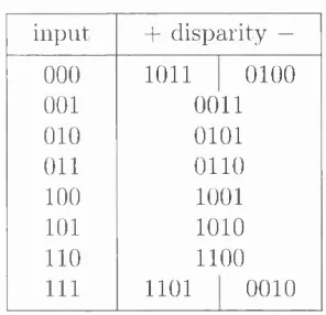
For the case where the number of bits n in the codeword is even, there exist words th a t have zero disparity. The transmission of such a word doesn’t affect th e running disparity, so it can be used in bo th dictionaries [33].
input + disparity —
000 1011 0100
001 0011
010 0101
Oil 0110
100 1001
101 1010
110 1100
111 1101 0010
Table 4.2: A 3B4B alternate line code employing zero disparity words in both dictionaries
tighter disparity bounds than the code in table 4.1 whose disparity is bounded by ±3.
o 0.: 0)
Q.
0.6
0.4
0.2
0.2 0.3 0.4
N o r m a lise d
0.5 0.6
N o r m a lis e d F r e q u e n c y
0.7 0.9
Figure 4.2: Frequency response of the 3B4B line code of table 4.2
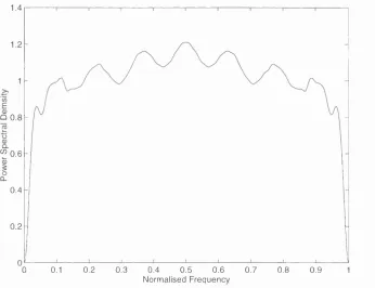
In figure 4.2 we see the frequency response of the 3B4B line code from table 4.2; this was obtained using the procedure described in [34, 35, 36, 37]. There is no DC component in the frequency response and the low frequency content is limited, the main objective which improves the immunity of the coded signal to inter-sym bol interference.
4 .4 Error co rrectin g lin e cod es
A common requirement in a coding system is to have bo th error protection and line coding properties.
Line encoder
Line decoder
ECC decoder ECC
encoder
Figure 4.3: A cascaded error control and line coding system
A commonly used arrangem ent in such a case is shown in figure 4.3. A line code is used to give the required line coding properties to the tran sm itted sequence, while an outer error control code is used to correct any errors th a t occur. There are two significant drawbacks in such a system. The first is th a t b o th codes add redundancy, and thereby the overall rate of the code may be significantly reduced. Furtherm ore, many line codes give rise to w hat is known as error extension: Since the line codes offer no error control, it is possible th a t an error th a t occurred in the channel will confuse the line decoder and will result in more errors th a t the error control code will have to correct.
have the desired line coding properties, while at the same tim e they are valid error correcting code words. Therefore, it is possible to effect the error correc tion before the line decoding, avoiding possible error extensions. Moreover, it is possible to achieve higher coding rates by using such codes,albeit potentially at the expense to some degree of the overall system complexity.
One such code th a t can be used when bounded disparity is desired together w ith error protection has been proposed[39] th a t partitions an error correcting code into two alternate dictionaries th a t have positive and negative disparity respec tively. The code used is a systematic linear transparent code and is divided in such a way th a t every code-word corresponds to its binary inverse in the alter nate dictionary. Using this partition scheme, one bit in the tran sm itted word is used to indicate whether the code-word has been inverted for transm ission, while the code-word is still valid.
To achieve higher efficiency, a scheme w ith more complicated encoding and decoding has also been proposed [40] where code-words th a t have zero disparity are used in b o th of the alternate dictionaries. Using this m ethod, the num ber of available entries in the dictionary increases.
4.4.1 Proposed technique.
is the previously nientioned teclini(iue, where both alternate code-words are the same, and therefore have zero Hamming distance.
110
Oil
010
000
101
100
001
Figure 4.4: The 3 bit code-word space
Figure 4.4 helps illustrate this point. Here, the eight possible 3 bit code-words are dis])layed as a cube. All code-words that have distance one are connected with a line. It is fairly easy to see that a disparity code with minimum Hamming distance two can only have three code-words.
010
Oil
000
001 101
110
100
However, we can select two alternate pairs, w ith each pair having distance two from the other pair, while the code-words of each pair have distance one. This is shown in figure 4.5, where each pair is connected w ith a thick line. This simple example is used to dem onstrate th a t higher rate codes are possible using this technique.
4.4.2 Example.
It is possible to design error correcting line codes th a t have more code-words pairs th a n the p artition into two sets of the longest possible error correcting code of the same length.
A more practical example is given in table 4.3. This is a 9 -b it distance 3 code where the possible number of pairs is 21. However, the maximum num ber of CO d e -words in a 9 -b it error correcting code is 40 [28]. Therefore this code can give error correcting line codes with more code-word pairs th an is possible using a norm al error correcting code. In the table, the pairs where the distance of the pairs is less th a n 3 are shown w ith an underlined word number. Only three of the 2 1 pairs meet the minimum distance constraint.
Figure 4.6 shows the power spectral density of this code.
word + disparity — 1 0 0 1 1 1 1 1 1 1 0 1 0 0 0 0 0 0 0 2 0 1 0 0 0 1 1 1 1 0 0 0 0 0 1 1 1 1 3 0 1 0 1 1 0 0 1 1 0 0 0 1 1 0 0 1 1 4 0 1 0 1 1 1 1 0 0 0 0 0 0 1 1 1 0 0 5 0 1 1 0 1 0 1 0 1 0 0 1 0 1 0 1 0 1 6 0 1 1 0 1 1 0 1 0 0 0 1 0 0 1 0 1 0 7 0 1 1 1 0 0 1 1 0 0 0 0 1 0 0 1 1 0 8 0 1 1 1 0 1 0 0 1 0 0 1 1 0 1 0 0 1 9 1 0 0 0 1 0 1 1 1 1 0 0 0 1 0 0 1 0 1 0 1 0 0 1 0 1 0 1 1 1 0 0 1 0 1 0 0 0 1 1 1 0 0 1 1 1 1 0 1 0 1 1 0 0 1 1 0 0 1 2 1 0 1 0 0 1 1 0 1 1 0 1 0 0 0 1 0 0 13 1 0 1 0 1 1 0 1 1 1 0 1 0 1 1 0 0 0 14 1 0 1 1 0 0 1 1 1 1 0 0 0 0 0 0 0 1 15 1 0 1 1 1 0 0 0 1 0 0 1 1 1 0 0 0 0 16 1 1 0 0 1 1 0 0 1 0 1 0 0 1 1 0 0 1 17 1 1 0 0 1 1 1 1 0 0 1 0 0 1 0 1 1 0 18 1 1 0 1 0 0 1 0 1 0 1 0 1 0 0 1 0 1 19 1 1 1 0 0 0 0 1 1 0 1 1 0 0 0 0 1 1 2 0 1 1 1 1 0 1 0 1 0 0 1 0 1 0 1 0 1 0 2 1 1 1 1 1 1 0 1 0 0 1 1 0 1 1 0 0 0 0
Table 4.3: An error correcting alternate line code w ith 9 bits and minimum distance 3. The underlined
words show the pairs with distance less th a t three
done w ith a similar procedure th a t selected words th a t had distance less th an three from their pair whenever possible. The whole procedure was repeated until no further improvement was obtained.
4.5 A sy m m e tr ic error co rrectin g cod es
û 0.
^ 0.6
0.4
0.2
0 0.1 0.2 0.3 0.4 0.5 0.6 0.7 0.8 0.9 1
N o r m a lis e d F r e q u e n c y
Figure 4.6: Frequency response of the new 9-l)it error correcting line code
disparity that can be alternatively used depending on the running disparity of the transniitted sequence.
The case where the asymmetric distance A is two (that is, single asymmetric Z channel error correcting codes), will be studied in more detail.
For a code with even word length, no improvement is possible with the proposed technicpie. Since the words with zero disparity can be transm itted in any case, the only improvement in code size would be possible if pairs of words with posi tive and negative disparity were possible with distance less than two. However, the difference in Hamming weight and the Hamming distance between the words of every possible pair are both greater than or equal to two. Therefore, from
the formula 2dA{a^b) = d,H(a,b) + \w{a) — w{b)\ we get th a t the asymm etric distance of the pair will be greater th an or equal to two.
However, in the case where the length of the code-words is odd, improvements are possible. It can be shown th a t any single asymmetric Z-channel error correcting code th a t consists of words of only positive (or negative) disparity can form one half of an alternate asymmetric Z-channel error correcting line code. Specifically, for two single asymmetric Z-channel error correcting codes, one w ith positive and one w ith negative disparity, a co de-word of one code will have distance less th an two w ith at most one code-word of the other code.
Assume three codewords c%, C2 and cg, w ith w{ci) < w{c2) < w{cs). Since
2dA{cL, b) = dnicL, b) \w{a) — w(b)\, we have th a t
2dA(ci, C2) +2dA(ci, C3) = d //(ci, C2) + d //( c i, C3)-\-w{c2)-w{ci)-\-w{c3)-w{ci).
However, d //(a, b) + d //(6, c) > d//(a, c) gives us
2dA(ci, C2) + 2dA(ci, C3) > d //(c2, C3) + w{c2) - w{ci) + w{cs) - w{ci) ^
<=> 2c/a(ci, C2) + 2dA(ci, C3) > 2d ^(c2, C3) + 2w{c2) - 2w{ci) <#>
dA(ci, C2) + dA(ci, C3) > dA(c2, C3) + w{c2) - w{ci).
If Cl has negative disparity, and C2, C3 have positive disparity, then w( c2) —
tu(ci) > 1 and since ^^(<^2, C3) > 2 we have
dA{ci,C2) + dA(ci,C3) > 3.
This helps the search for asymmetric Z-channel error correcting line codes with asymmetric distance at least 2 and an odd word length. For example the pro cedure that was described earlier can be used with the simplification th at only the positive disparity set needs to be searched since the existence of a negative counterpart is guaranteed. Assuming the code with the most code-words is found, a code with the same size but negative disparity words can be generated by inverting all words. Then all pairs of distance less than two can be identified, and the remaining code-words can be paired arbitrarily. The search space can be reduced further by employing the properties of the asymmetric Z-channel error correcting codes discussed in the previous chapter. The all one codeword and two other codewords of weight n — 2 can be selected as parts of any code, simplifying the search.
Q 0.
w 0.6
0.4
0.2
0.2 0.3 0.4
N o r m a lis e d
0.5 0.6
N o r m a lis e d F r e q u e n c y
0.7 0.9
Figure 4.7: Power spectral density of the new 1 1-bit asymmetric Z-channel error correcting line code
( 0 5 f , 0 0 0 ) , ( 0 b 7 , 0 0 3 ) , ( Oe b , OOc ) , ( O f c , 1 2 0 ) , ( O f f , 5 0 6 ) , ( 1 2 f , 4 1 0 ) ,
( 1 7 3 , 1 3 3 ) , ( 1 7 d , 2 e 4 ) , ( 1 9 d , 0 9 d ) , ( l b a , 2 8 0 ) , ( I c 7 , 0 c 7 ) , ( l d b , 6 4 5 ) ,
( l e e , 4 b 2 ) , ( 2 3 b , 2 2 8 ) , ( 2 6 7 , 0 3 2 ) , ( 2 7 0 , 5 5 2 ) , ( 2 9 0 , 2 9 6 ) , ( 2 a d , l l l ) ,
( 2 c f , 6 8 2 ) , ( 2 d 5 , 0 4 9 ) , ( 2 f 2 , 4 0 5 ) , ( 2 f 9 , 4 e 8 ) , ( 3 1 7 , 0 6 4 ) , ( 3 3 f , l 0 O ) ,
( 3 4 d , 4 c O ) , ( 3 5 a , 3 1 a ) , ( 3 6 b , 1 1 c ) , ( 3 7 4 , 3 7 0 ) , ( 3 8 b , 2 5 0 ) , ( 3 a 6 , 0 9 8 ) ,
( 3 b l , 3 9 1 ) , (3 b c ,4 7 4 ), ( 3 d 6 , 3 2 c ) , ( 3 e 8 , 1 4 2 ) , ( 3 0 f , l b 4 ) , ( 3 f 5 , 4 4 3 ) ,
( 3 f a , 3 8 8 ) , ( 4 3 d , O a l ) , ( 4 6 e , 4 4 e ) , ( 4 7 7 , 6 d 0 ) , ( 4 8 f , 4 8 b ) , ( 4 b b , 5 9 8 ) ,
( 4 d 3 , 7 0 0 ) , ( 4 d d , 5 0 d ) , ( 4 e 5 , 4 a 5 ) , ( 5 1 b , 2 0 6 ) , ( 5 3 6 , 4 0 a ) , ( 5 4 f , 4 5 9 ) ,
( 5 5 5 , 1 5 5 ) , ( 5 6 9 , 5 6 1 ) , ( 5 7 a , 2 5 c ) , ( 5 7 f , O f l ) , ( 5 9 0 , 2 3 5 ) , ( 5 a 3 , 1 8 4 ) ,
( 5 a c , 0 1 b ) , ( 5 a f , 3 4 4 ) , ( 5 b 5 , 7 0 3 ) , ( 5 c a , 4 9 4 ) , ( 5 d 7 , 0 d a ) , ( 5 f 0 ,0 5 6 ) ,
( 5 f 9 , 6 1 1 ) , ( 6 1 f , 5 c 4 ) . ( 6 4 b , 5 3 0 ) , (6 5 6 ,0 7 8 ), ( 6 6 d , 5 2 a ) , ( 6 7 1 , 2 6 1 ) ,
(67b,2bO ), ( 6 9 9 , 0 a 6 ) , ( 6 a a , 2 a a ) , ( 6 b 4 , 2 8 5 ) , ( 6 b d , 1 9 2 ) , ( 6 c c , 6 8 c ) ,
( 6 d a , 4 1 7 ) , ( 6 d f , l a 9 ) , ( 6 e 3 , 3 c 2 ) , ( 6 e e , 0 3 e ) , ( 7 0 0 , O c c ) , ( 7 2 5 , 7 a 0 ) ,
( 7 3 3 , 2 c 9 ) , ( 7 3 8 , 6 3 8 ) , ( 7 5 9 , 2 5 3 ) , ( 7 5 0 , 3 2 2 ) , ( 7 6 2 , 6 6 2 ) , ( 7 6 7 , 5 8 1 ) ,
( 7 8 7 , 2 0 f ) , ( 7 9 2 , 7 4 8 ) , ( 7 9 b , 6 2 4 ) , ( 7 a 9 , 4 2 9 ) , ( 7 b 6 , 2 4 a ) , ( 7 c l , 7 1 4 ) ,
( 7 c d , 0 6 d ) , ( 7 e 4 , 1 2 5 ) , ( 7 f 3 , 1 8 e ) , ( 7 f c , 1 6 6 ) , ( 7 f f , 1 4 b )
Table 4.4: New 11-b it single asymmetric Z-channel error correcting line code with 95 code-word
pairs (in hexadecimal). Underlined are the pairs w ith asymmetric distance less th a n two
This code was generated with the above procedure, with an added step. After a code of 94 code-words was generated, an added optimisation step was used. This tried to improve all subsets of the code with size 94 — k, where k was progressively increased, by exhaustively searching all possible combinations of the remaining words with positive disparity. The result of 95 words was obtained for k = 5. For values of k higher than 6 this optimisation was found to be computationally infeasible.
o 0.,
CL
W 0.6
0.4
0.2
0.4 0.5 0.6
N o r m a lis e d F r e q u e n c y
0.7 0.9
0.1 0.2 0.3
Figure 4.8; Power spectral density of the reduced 11-b it asymmetric Z-channel error correcting line code
This code can be transformed to satisfy a tighter disparity bound, by removing the all one and all zero code-words. The power spectral density of the resulting 94 word code is shown in figure 4.8, where a small reduction of the low frequency content can be seen.
4.5.1 Alternative encoding scheme.
Another improvement that recpiires more complicated encoding is possible using a technicjue similar to that described in [9]. This requires that the code-words are paired in such a way that words with high positive (negative) disparity are ])aired with words with low negative (positive) disparity. The encoder can then select the code-word that gives a value of disparity closer to zero which on occasion will have the same sign as the running disparity. A small example will illustrate the point. If the current disparity is —1 and the words in the pair that is to be transm itted have disparities of +7 and —1, selecting based on the sign the disparity would become +6, while selecting the other one the disparity
becom es —2.
0.4
0.2
0 0.1 0.2 0.3 0.4 0.5 0.6 0.7 0.8 0.9 1
N o r m a lis e d F r e q u e n c y