Microalgae classification using semi-supervised and active learning based on Gaussian mixture models

(1)

DOI 10.1007/s13173-013-0121-y O R I G I NA L PA P E R

Microalgae classification using semi-supervised and active

learning based on Gaussian mixture models

Paulo Drews-Jr. · Rafael G. Colares · Pablo Machado · Matheus de Faria· Amália Detoni· Virgínia Tavano

Received: 12 November 2012 / Accepted: 16 August 2013 / Published online: 8 September 2013 © The Brazilian Computer Society 2013

Abstract Microalgae are unicellular organisms that have different shapes, sizes and structures. Classifying these microalgae manually can be an expensive task, because thousands of microalgae can be found in even a small sample of water. This paper presents an approach for an automatic/semi-automatic classification of microalgae based on semi-supervised and active learning algorithms, using Gaussian mixture models. The results show that the approach has an excellent cost-benefit relation, classifying more than 90 % of microalgae in a well distributed way, overcoming the supervised algorithm SVM.

Keywords Active learning·Semi-supervised learning· Microalgae classification

1 Introduction

Microalgae are unicellular organism that can be found in a variety of sizes, structures and forms. These characteristics allows us to classify microalgae into different phytoplankton taxonomic groups. Microalgae classification is relevant to biology and oceanology, because the description of

microal-P. Drews-Jr. (

B

)·P. Machado·M. de Faria

Centro de Ciências Computacionais, Universidade Federal do Rio Grande (FURG), Rio Grande, RS, Brazil

e-mail: [email protected] R. G. Colares

Departamento de Ciência da Computação, Universidade Federal de Minas Gerais (UFMG), Belo Horizonte, MG, Brazil e-mail: [email protected]

A. Detoni·V. Tavano

Instituto de Oceanografia, Universidade Federal do Rio Grande (FURG), Rio Grande, RS, Brazil

gae species at a certain time and place is important to the understanding of how energy is transferred from the food

chain base to higher trophic levels [5]. Furthermore, it reflects

changes in fish stocks and the carbon cycle of a given environ-ment. The classification of microalgae and characterization of the predominant taxonomic groups has a diversity of appli-cations, such as understanding of a phytoplankton

commu-nity’s structure. A recent census of marine life [4] gathered

research from more than 80 nations, and lasted one decade, in order to obtain a global benthic biomass map predicted to the seafloor, phytoplankton included.

Microalgae are classified in groups based on different characteristics, with huge morphological variations such as round, oval, cylindrical, and fusiform cells, as well as projec-tions like thorns, cilia, etc. In addition to the taxonomic clas-sification, phytoplankton organisms can be classified

accord-ing to their sizes: picoplankton (0,2–2 µm), nanoplankton

(2–20µm), and microplankton (20–200µm). Specific

com-position, size structure and biomass studies about phyto-plankton communities are being developed through the

clas-sic method of optic microscopy [13], in which an observer

has to manually manipulate a small water sample requiring more than a day for a complete analysis.

(2)

The proposed approach combines two types of learning: semi-supervised and active. The first assumes that only a small part of data has known ranking a priori, and tries to use information from non-ranked data to improve the clas-sification. The second, active, searches the non-ranked data for the one that provides the most information gain, and then asks the user the rank of that data. In this work, both learning types were combined to improve microalgae classification. The process is initialized with semi-supervised learning, and then is improved using active learning.

In order to acquire the microalgae data, a FlowCAM

par-ticle analyzer [15] was used. It is capable of obtaining

infor-mation concerning microorganism in water samples. Four experts analyzed and ranked the obtained data in order to validate the proposed approach.

2 Related work

Most studies found in the literature try to classify plankton, which, although not exactly the focus of this work, shares

some similarities with our goal. Blaschko et al. [1] presented

a comparison of supervised approaches to learning and classi-fying plankton. Those approaches are used to classify larger organisms than the targets of this work, thus presenting a greater number of relevant features, facilitating the learn-ing process. Furthermore, those approaches used extensive supervised data, which makes it very costly and not

extensi-ble. Finally, Blaschko et al. [1] also used the FlowCAM and

the best results obtained were around 70 %.

Another work of interest was proposed by Xu et al. [21],

which uses a restrict set of supervised data classified with a SVM classifier, using non-ranked data to improve the learn-ing. Although the presented approach is adequate to this work, it does not use experts as an information source. They obtain the information through a density method technique, which is sensitivity to the microalgae size. Due to the small size of the microalgae used in this study, the amount of infor-mation is reduced, which makes this approach unfeasible.

The work of Sosik and Olson [19] used the FlowCytobot

equipment to extract features from the phytoplankton, on a similar process to the FlowCAM. The results obtained in the automatic classification were around 68 and 99 %, depending on the type of organism that were classified. They obtained least significant results to smaller plankton, the focus of this work.

Another work from Hu and Davis [14] usesco-occurrence

matrices techniques and SVM to classify plankton. Using both supervised learning techniques, they obtained around 72 % of accuracy.

The problem of classification of microalgae was addressed

in the work of Drews, Jr., et al. [9], where Gaussian

mix-ture models were used together with semi-supervised and

active learning. The present work is an extension of the pre-vious work, where the methodology is detailed. Furthermore, we present and discuss a more thorough experimental data acquired using FlowCAM.

3 Methodology

As explained on Sect.1, this work uses an approach based

on the combination of two learning types: semi-supervised and active, with the objective to classify microalgae. The first step of the work was to obtain the data of the microal-gae using the FlowCAM. Given a water sample, this equip-ment is capable of finding and analyzing microalgae in order to identify up to 26 different features to compose the data-bases used in this work. This work used only seven of these features: ESD diameter, ESD volume, width, length, aspect ratio, transparency, and CH1 peak.

We selected the best of these features using the approach

proposed by Peng et al. [16]; the method is an optimal

first-order approximation of the mutual information criteria. The selected features are in accordance with FlowCAM software

manual [11], which defines these seven features as good

fea-tures in general cases. Four experts analyzed and classified these datasets in order to generate a ground truth to validate

the proposed approach. Fig.1shows the FlowCAM interface.

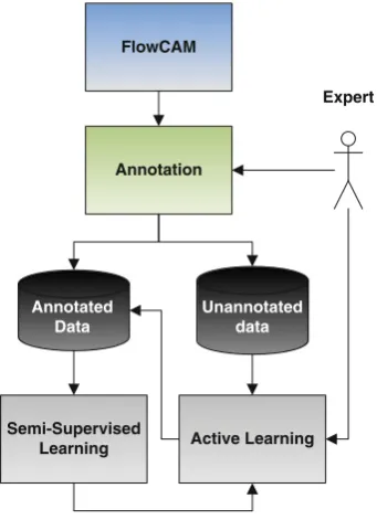
The first step of this proposed method is the development of a semi-supervised algorithm to classify the microalgae. IN this step, the algorithm receives as input just a small sample of ranked data, wherein at least one instance of each class needs to be provided. This allow that the algorithm is able

(3)

FlowCAM

Annotated Data

Unannotated data

Annotation

Semi-Supervised

Learning Active Learning Expert

Fig. 2 Proposed approach

to identify and cluster microalgae with similar characteris-tics, creating a model of the microalgae class. This model allows new instances, non-ranked, to be observed and classi-fied through their characteristics, updating the model simul-taneously.

When the semi-supervised algorithm finishes, the active algorithm analyzes the instances that were not ranked and searches among them for the one that provides the largest information gain for the model. In order to identify which

instance this is, three methods were used:least confident

sam-pling,margin samplingandentropy-based sampling. Then, the chosen instance is presented to the user, who will indi-cate the class to which it belongs. This class is incorporated into the model, which is then updated and tries to classify the other non-ranked instances. This process is repeated as long as the user finds it to be favorable or until the information

gain is too small. Figure2illustrates the described process.

In the following sections, we describe the semi-supervised and active learning algorithms.

3.1 Semi-supervised learning

Due to the nature of the data used on this work, where the instances have similar characteristics when they belong to the same class, it is costly to rank a large set of instances. Thus, it favors an approach that uses clustering to classify microalgae. Furthermore, as the number of classes, species

of microalgae on a sample are known and small,1 and the

1_{This size is dependent of the environment. Typically, we have around}

ten different classes.

classes are relatively well separated, the use of theGaussian

mixture model(GMM) withexpectation-maximization(EM)

becomes a natural choice [7].

3.1.1 Gaussian Mixture Models

The Gaussian mixture model (GMM) is a probability den-sity function (PDF) given by a linear combination of a Gaussian PDF. More specifically, the function is a mixture of a Gaussian PDF if it has the following form:

p(x|K, θ)=

K

k=1

πkN(x|μk,k), (1)

where K is the number of the Gaussian PDF andπk is the

weight of each one in the mixture. This weight can be inter-preted as the a priori probability that the random variable

value was generated by the Gaussiank.

Considering, 0 ≤πk ≤ 1 and

K

k=1πk = 1, the GMM

can be defined by the parameter listθ, which represents the

parameters from each Gaussian and their respective weights,

i.e.,θ= {π1, μ1,1, . . . , πK, μK,K}, whereμandare

the mean and the covariance matrix, respectively.

The problem with estimating the Gaussian mixtures lies in

determiningθ, given that onlyKand the data are known and

the other parameters are unknown (πkandθk =(μk,k)).

ConsideringY = {y1, . . . ,yn, . . . ,yN}with yn ∈ RM,

the independent sample set, whereM is the size of the data

sample space andN is the number of samples. In this work,

ynrepresents the dataset instances, the microalgae. It is

pos-sible to estimate the probability p(yn|K, θ)directly for each

K. However, a logarithmic function of the probability is

nor-mally used for ease of handling numbers. Thus, we have:

ˆ

θ=argmax

θ,K

logp(y|K, θ). (2)

Solving the Eq.2is not an easy task [8,10]. The number

of variables to be estimated can grow exponentially with the

size of K andθ, thus making the computation very costly.

We used the EM algorithm to solve this problem.

3.1.2 EM algorithm

The EM algorithm is used to determine the class of each data

[7]. The algorithm aims to solve problems in which we do

not know all the information needed for the solution. The algorithm is composed of two steps:

E-step: On this step, the missing data are estimated using the observed data and the actual status of the model para-meters.

(4)

The EM algorithm seeks to classify theyndata on classes,

or Gaussian, and, later, to re-estimate each class value. Using

Bayes’ rule the probability that a pointynbelongs to classkis

computed. Consideringθ(i)to be theθvalue on the iterative

stepiof the algorithm and known in this step, the probability

ofE-stepis given by:

p(k|yn, θ(i))=

πk·N(yn|θk(i))

K

l=1πl·N(yn|θ_l(i))

. (3)

Calculating these probabilities makes it possible to

esti-mateθandπ. These equations below show how each value

is estimated in the maximization step (M-step). First, one

normalizing parameterNkis estimated by the posterior

esti-mation of new values forπk, μk,k. From this, the update

equations from step M can be defined:

Nk = N

n=1

p(k|yn, θ(i)), (4)

πk =

Nk

N , (5)

μk =

1

Nk N

n=1

ynp(k|yn, θ(i)), (6)

k =

1

Nk N

n=1

(yn−μk)·(yn−μk)Tp(k|yn, θ(i)). (7)

The algorithm initialization is critical for a good

perfor-mance, i.e., theθ(0). In this work, the initialization is done

based on the ranked data available, generating a initial model using random initialization. Thereafter, using non-ranked data information, this model is updated. This approach has the major advantage of ensuring that data labeled as distinct classes remain this way.

The approach of Zhu and Goldberg [22] was used to

esti-mate the GMM model from ranked and non-ranked data. The ranked data are computed distinctly in the E-step. This way, the ranked data have their probability set to 100 % for their class and 0 % to the other classes.

3.2 Active learning

After executing the semi-supervised learning algorithm, it is possible to divide the dataset into two groups: ranked

instances and non-ranked instances. Considering X =

{x1, . . . ,xn, . . . ,xN}as the set of non-ranked instances andk

the possible classes, the active algorithm must find anxi ∈ X

that maximizes the amount information added to the system

when it is classified askj.

In order to define which instancexi is going to be

pre-sented to the user, three metrics were used to calculate the information contained therein. The three metrics, based

on the work of Settles [18] and Friedman et al. [12], are

described below:

1. Least-confident sampling: involves choosing the instance with the least probability of belonging to the class with

the most probability. The instancex to be chosen is the

one that:

x=argmin

i

p(zi = ˆk|xi) (8)

wherekˆ=argmaxk p(zi =k|xi)is the class with most

probability.

2. Margin sampling: involves choosing the instance with the least margin between the class with most probability and

the one with the secondmost probability. The instancex

to be chosen is the one that:

x=argmin

i

[p(zi = ˆk1|xi)−p(zi = ˆk2|xi)] (9)

wherek1ˆ andk2ˆ are the most likely classes.

3. Entropy-based sampling: involves choosing the instance with the most entropy of the classes’ probabilities. The

instancexto be chosen is the one that:

x=argmax

i

−

k

p(zi=k|xi)log p(zi =k|xi) (10)

After defining which instance is the most informative, the user must inform the system its rank. This classification is used by the EM algorithm in order to find the best model for the data, ranked or non-ranked, with this new information. Such model is initialized with the best representation until the present moment.

4 Experimental results

The results were obtained using two different datasets acquired using the FlowCAM equipment. The Oceano-graphic Institute of FURG collected the data during an oceanographic expedition on the Atlantic Ocean in different place and depth. In order to validate the results, four different experts classified these datasets. Doubtful data were

elimi-nated, typically they were small microalgae, around 1µm, or

really big microalgae, which were problems on the

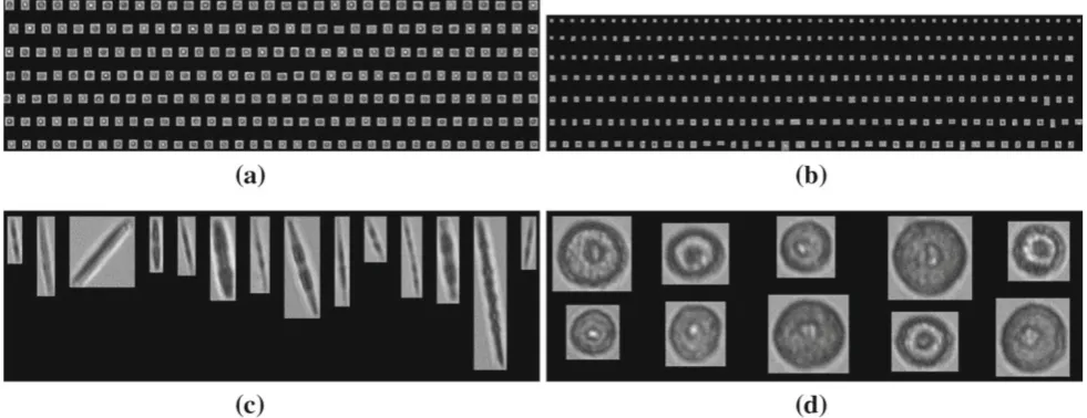
acquisi-tion by the FlowCAM or were microalgae colonies. Figure3

illustrates some excluded data during the process.

The first dataset was classified on four different classes:

flagellates (Fig. 4a), mesopores (Fig.4d), pennate diatoms

(Fig.4c) and others (Fig.4b). An important characteristic,

usually found in this kind of data, is the unbalance of classes. The flagellates and the others classes represent more than

(5)

Fig. 3 Some examples of microalgae acquired by FlowCAM that were excluded due to acquisition problems or the presence of microalgae colonies. The presence of colonies is due to a failure in the segmentation process of FlowCAM. These fail are common due to the acquisition process of the FlowCAM device

are reduced size data with few characteristics, which makes the classification problem difficult to solve.

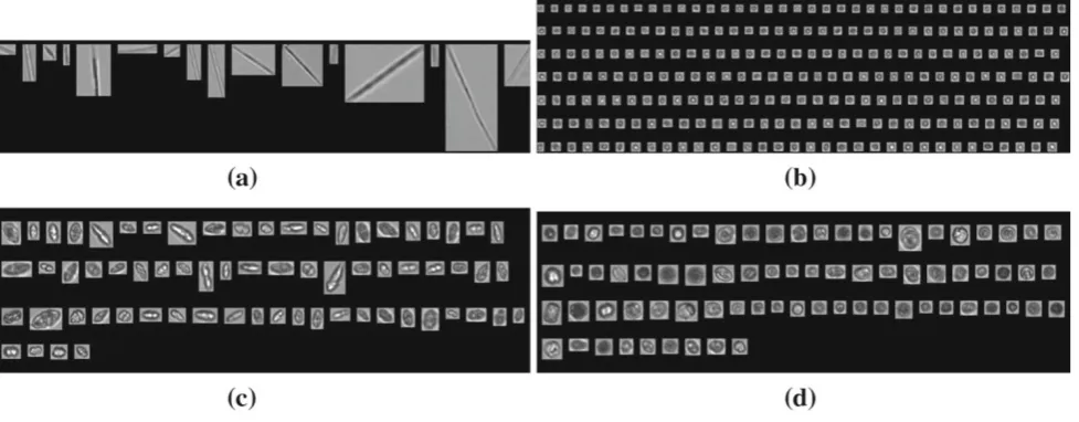
The second dataset was classified on four different classes:

pennate diatoms (Fig.5a), flagellates (Fig.5b), gymnodinium

(Fig. 5c) and prorocentrales (Fig. 5d), respectively. Both

datasets have two similar species of microalgae and two different ones. This is due to different place and, mainly, depth where the samples were acquired. The characteristics of the data are similar, both datasets are unbalanced and with reduced size data.

In order to validate the proposed approach, we used some evaluation metrics. As there are multiple classes, the

metrics need to deal with this kind of information. It was

used the F-score metric [17], defined by the Eq.11, which is

the harmonic mean between the recall(r)and the precision

(p),defined by Eq.12.

F_β =(1+β) pr

(β2_p₎₊_r, (11)

whereβis a constant factor. At the present work,βwas equal

to 1, obtaining the F1-score metric.

rk =

T pk

T pk+F pk,

pk=

T pk

T pk+F nk,

(12)

where,T pkis the number of correctly classified microalgae

for classk;F pkis the number of false positives, the number

of microalgae that were wrongly classified as classk;F nkis

the number of false negatives, the number of microalgae that

are from classk, but were defined to another class;kis the

microalgae class. These metrics are defined for each class.

The F1-score values are defined on the interval(0,1), and

if they are near one they represent a better classification, while small values, near zero, represent a low classification quality. However, to evaluate the performance for all classes was used the micro-averageandmacro-averagemetrics [20]. These metrics evaluate the average performance of the classifier,

based on precision and recall metrics. Themacro-average

metric gives an average where every class is treated with same

importance, while themicro-averagemetric gives an average

where the microalgae are treated with the same importance. It is important to evaluate these two metrics due the

fact that the micro-averageis more influenced by the

clas-sifier performance on classes with large samples, while the macro-averageis more influenced by classes with less

Fig. 4 Examples of the four classes of microalgae acquired by Flow-CAM on the first dataset. This dataset were classified on four different classes:aflagellates,cpennate diatoms,dmesopores, andbothers.

(6)

Fig. 5 Examples of the four classes of microalgae acquired by Flow-CAM on the second dataset. This dataset were classified on four dif-ferent classes:apennate diatoms,bflagellates,cgymnodinium and

dprorocentrales. As in the previous figure, it shows some important characteristics of this data as the unbalance and the reduced informa-tion about each microalgae

samples. Thus, using both metrics, the F1-score was

evalu-ated. It is called maxF1 when obtained usingmacro-average

and minF1 when obtained usingmicro-average. In the case of

multiple classes, the minF1 has the same value as the metric

known as accuracy (Ac), which is defined by Eq.13. Thus,

this work uses these two metrics: accuracy, or minF1, and maxF1.

Ac=

kT pk

N , (13)

whereN is the total number of samples on the data base and

kis the sum for all classes.

Some results were obtained in order to validate the approach using these two datasets completely classified. The first dataset is composed by 1,526 microalgae divided into four classes, as previously described, each one with 1,003 (Flagellates), 500 (others), 14 (pennate diatoms) and 9 sam-ples (mesopores). The second dataset is composed by 923. It is also divided in four classes, as previously described, each one with 112 (Pennate Diatoms), 669 (Flagellates), 65 (gymnodinium) and 77 samples (prorocentrales).

From these datasets, smaller classified bases were ran-domly generated, with approximately 1, 3, 5, 10, 20 and 50 % of the original dataset, where each class should have at least one sample. In order to obtain quantitative results, for each percentage were generated ten different instances. Forty-eight samples were actively selected and classified.

4.1 Evaluation of the active learning

Firstly, the active learning capabilities were evaluated using

three different metrics: Least Confidence Sampling,

Mar-gin Sampling e Entropy, when compared with a random

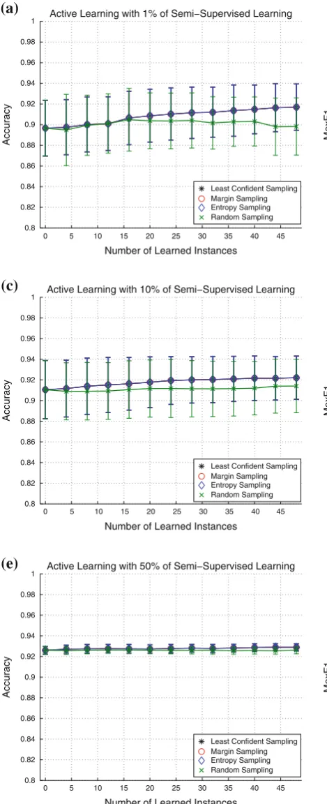
selection. The results obtained in the first dataset is shown

in Fig. 6. It shows the results for 1, 10 and 50 % of

ini-tial supervision using both evaluation metrics: Accuracy and maxF1.

Figure6a and b show the results for 1 % of initial

semi-supervision, in which the random selection presents a small accuracy and maxF1 raises with the addition of new sam-ples. On the other hand, the other metrics had a significant improvement, especially on accuracy, which means a better classification independently of the classes.

On Fig.6c and d, the results for 10 % of initial

supervi-sion are shown. It can be noted that the accuracy starts at a higher value than 1 % of semi-supervision and increases smoother for all metrics and the random selection. For the results obtained with 50 %, the variance is even smaller, as

shown in Fig. 6e and f. Moreover, in this case, the active

learning presents a small improvement for accuracy and maxF1.

The random selection can be seen as a semi-supervised addition of samples, thus, it can be noted that the active learn-ing represents a significant gain, especially when there is little initial information.

Considering the second dataset, the results are similar to the ones obtained with the first dataset. One important differ-ence between the datasets is the mean of accuracy and maxF1. The second dataset has different classes of microalgae, and the intraclass variability is larger than the first dataset. Thus, it is hardier to classify.

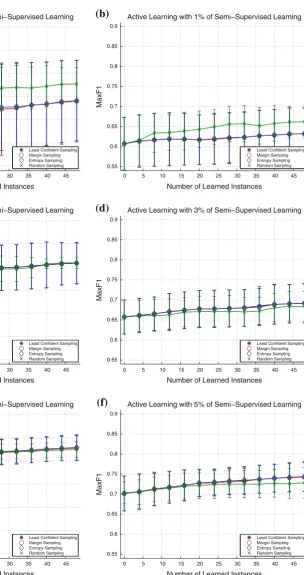
Figure7shows the results for 1, 3 and 5 % of initial

super-vision. It is interesting to see in Fig.7a and b that the random

(7)

0 5 10 15 20 25 30 35 40 45 0.8

0.82 0.84 0.86 0.88 0.9 0.92 0.94 0.96 0.98

1 Active Learning with 1% of Semi−Supervised Learning

Accuracy

Number of Learned Instances

0 5 10 15 20 25 30 35 40 45 0.8

0.82 0.84 0.86 0.88 0.9 0.92 0.94 0.96 0.98

MaxF1

0 5 10 15 20 25 30 35 40 45 0.8

0.82 0.84 0.86 0.88 0.9 0.92 0.94 0.96 0.98

Accuracy

Least Confident Sampling Margin Sampling Entropy Sampling Random Sampling

0 5 10 15 20 25 30 35 40 45 0.8

0.82 0.84 0.86 0.88 0.9 0.92 0.94 0.96 0.98

MaxF1

0 5 10 15 20 25 30 35 40 45 0.8

0.82 0.84 0.86 0.88 0.9 0.92 0.94 0.96 0.98

Accuracy

0 5 10 15 20 25 30 35 40 45 0.8

0.82 0.84 0.86 0.88 0.9 0.92 0.94 0.96 0.98

MaxF1

Fig. 6 Comparative of active learning metrics against a random selec-tion using thefirst dataset, with results showing mean and standard deviation for the datasets with ten different bases.The vertical axis represents the accuracy andthe horizontal axisrepresents the num-ber of active samples informed to the system.aAccuracy for 1 % of

initial semi-supervision,bMaxF1 for 1 % of initial semi-supervision,c

accuracy for 10 % of initial semi-supervision,dMaxF1 for 10 % of ini-tial semi-supervision,eaccuracy for 50 % of initial semi-supervision,

(8)

0 5 10 15 20 25 30 35 40 45 0.65

0.7 0.75 0.8 0.85 0.9 0.95

Active Learning with 1% of Semi−Supervised Learning

Accuracy

0 5 10 15 20 25 30 35 40 45 0.55

0.6 0.65 0.7 0.75 0.8 0.85 0.9

MaxF1

0 5 10 15 20 25 30 35 40 45 0.65

0.7 0.75 0.8 0.85 0.9 0.95

Accuracy

0 5 10 15 20 25 30 35 40 45 0.55

0.6 0.65 0.7 0.75 0.8 0.85 0.9

MaxF1

0 5 10 15 20 25 30 35 40 45 0.65

0.7 0.75 0.8 0.85 0.9 0.95

Accuracy

0 5 10 15 20 25 30 35 40 45 0.55

0.6 0.65 0.7 0.75 0.8 0.85 0.9

MaxF1

Fig. 7 Comparison of active learning metrics against a random selec-tion using thesecond dataset, with results showing the average and standard deviation for the datasets with ten different instances.The ver-tical axisrepresents the accuracy andthe horizontal axisrepresents the number of active samples informed to the system.aAccuracy for 1 % of

initial semi-supervision,bMaxF1 for 1 % of initial semi-supervision,

caccuracy for 3 % of initial semi-supervision,dMaxF1 for 3 % of initial semi-supervision,eaccuracy for 5 % of initial semi-supervision,

(9)

the active learning. The main reason for these results is due the large intraclass variance in this dataset. Thus, the sys-tem is not able to classify with a small number of supervised samples. In this case, the statistical selection falls into “local minima”. In this case, the random selection chooses samples that improve the results, while the statistical methods choose samples that obtain a small improvement in relation to the random one.

In Fig.7c and d, the results obtained by all selection

meth-ods are similar, with the maxF1 metrics of the random selec-tion being worse than the others are. Considering 5 % of initial supervision the statistical methods are better than

ran-dom selection, as shown in Fig.7e and f. This results remain

to the 10, 20 and 50 %. The entropy based sampling obtains a small advantage to the other metrics in all cases.

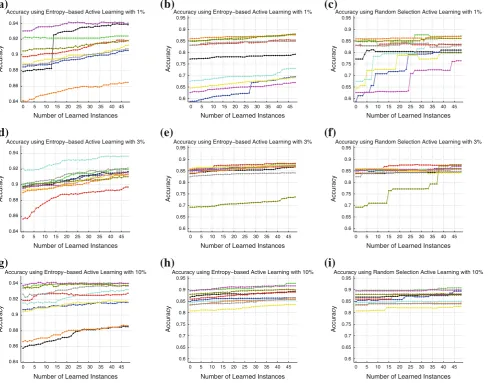
Figure8 shows the results for accuracy of each of the

ten generated bases from both datasets, considering a semi-supervision of 1, 3 and 10 %. The vertical axis represents the accuracy and the horizontal axis represents the number of active samples informed to the system. The accuracy results for the semi-supervised learning can be seen at number zero of the horizontal axis. As expected, the results shows that with a small semi-supervision, the accuracy is ruled by the chosen samples, and as the number of active samples increases, the variance decreases. The first two columns in this figure show the results using entropy for both datasets, and the last column using random selection for the second dataset.

On Fig.8a and b, it is possible to see the difference in

accu-racy obtained by the proposed methodology for both dataset using 1 % of supervision. The second dataset is hardier to classify, thus the results show bases with approximately 65 % in accuracy. In these two figures is possible to see an inter-esting characteristics of 1 % supervision, some samples are capable to improve the accuracy in more than 5 %, as the

base in black in Fig.8a and in blue in Fig.8b.

This phenomenon also happens, in Fig.8c, in a large scale,

where the random selection is used. It mainly occurs in bases where the initial accuracy is smaller. Thus, this base is com-posed by unrepresentative instances. Therefore, a represen-tative sample can improved the capability of the system to classify correctly the unclassified data. It explains the results

obtained in the Fig.7a and b.

Figure8d and e show the results for each base,

consider-ing 3 % of supervision. In this case, the first dataset shows a better accuracy value than the second dataset. The char-acteristics of the results are similar, with almost all bases with a small increasing in the accuracy with the active learn-ing. Moreover, both results presents a base with small initial accuracy. This base, as previously explained, is sensible to random selection that generated some steps in the accuracy,

as shown in Fig.8f. The other bases are less sensible to the

random selection, where the increasing in the accuracy is almost zero for the random selection, by the other side; the

entropy based sampling is able to select good samples that increases the accuracy.

On Fig.8d, there are two extreme cases. The first one, on

cyan, 92 % of accuracy is obtained with a small supervision, while, on the second one, on red, only 86 % of accuracy is obtained. It can be noted that all instances had an improve-ment when new samples are actively selected. This is clearer on the red instance that goes from 86 % to almost 90 %. This fact also occurs in both datasets.

The results obtained using 10 % of supervision with

entropy selection is shown in Fig. 8g and h. As seen in

the previous results, the first dataset present a better accu-racy than second dataset. The new actively selected samples improve in a small way the classification. This is due to a small capacity of generalization for this big group of sam-ples, which means that new samples adds little information.

It is also possible to see in Fig. 8i, the random selection

presents a very small improvement in the accuracy. In this case, there are only a small number of informative samples to be selected, and the random method has a small chance of selecting them. Although these facts, the entropy- based sam-pling select informative samples. It is shown by the increasing

in the accuracy of almost all bases, in Fig.8g and h.

In order to evaluate whether the obtained performance was adequate, the results were compared with the support vector

machine (SVM) [3] algorithm. This algorithm is considered

the state-of-art on supervised learning and classification. The

libSVM implementation [2] was used with a radial base

ker-nel function, which presented better results. All other para-meters were kept to its default.

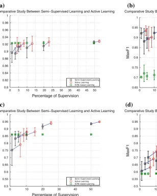
Figure9shows the results including the active learning as a

supervision addition. In black are shown the results obtained using only semi-supervised learning. The results after using the active learning are shown in red, which makes the super-vision percentage to be raised. The blue line links the data used on the initialization of the active learning after forty-eight instances, in percentage.

Figure9a and b shows semi-supervised learning, active

learning using entropy and SVM learning results to accu-racy and MaxF1 metrics for the first dataset. It can be noted that SVM has a small accuracy improvement with the increase of supervision, although it has better results than the supervised algorithm alone. Only for 50 % of semi-supervision the presented approach obtains a better accu-racy, while the active learning has similar results to the ones obtained by SVM.

(10)

0 5 10 15 20 25 30 35 40 45 0.84

(a)

(b)

(c)

(d)

(e)

(f)

(g)

(h)

(i)

0.86 0.88 0.9 0.92 0.94

Accuracy using Entropy−based Active Learning with 1%

Accuracy

0 5 10 15 20 25 30 35 40 45 0.6 0.65 0.7 0.75 0.8 0.85 0.9 0.95

Accuracy

0 5 10 15 20 25 30 35 40 45 0.6 0.65 0.7 0.75 0.8 0.85 0.9 0.95

Accuracy using Random Selection Active Learning with 1%

Accuracy

0 5 10 15 20 25 30 35 40 45 0.84 0.86 0.88 0.9 0.92 0.94

Accuracy

0 5 10 15 20 25 30 35 40 45 0.6 0.65 0.7 0.75 0.8 0.85 0.9 0.95

Accuracy

0 5 10 15 20 25 30 35 40 45 0.6 0.65 0.7 0.75 0.8 0.85 0.9 0.95

Accuracy

0 5 10 15 20 25 30 35 40 45 0.84 0.86 0.88 0.9 0.92 0.94

Accuracy

0 5 10 15 20 25 30 35 40 45 0.6 0.65 0.7 0.75 0.8 0.85 0.9 0.95

Accuracy

0 5 10 15 20 25 30 35 40 45 0.6 0.65 0.7 0.75 0.8 0.85 0.9 0.95

Accuracy

Fig. 8 Evaluation of the different instances of the semi-supervised data. In order to obtain statistical results, we generated ten different instances for each supervision percentage. The accuracy for all ten instances is shown using the proposed method with entropy, in the first two columns, and random selection, in the last column. The visual-ization is improved using different colors.the vertical axisrepresents the accuracy andthe horizontal axisrepresents the number of active samples informed to the system. It is important to call attention to the vertical axis, where the intervals are different between the results from

the first and the second datasets.aResults for 1 % of semi-supervision in thefirst dataset.bResults for 1 % of semi-supervision in thesecond dataset.cResults for 1 % of semi-supervision in thesecond dataset.

dResults for 3 % of semi-supervision in thefirst dataset.eResults for 3 % of semi-supervision in thesecond dataset.fResults for 3 % of semi-supervision in thesecond dataset.gResults for 10 in thefirst dataset.hResults for 10 % of semi-supervision in thesecond dataset.i

Results for 10 % of semi-supervision in the second dataset (color figure online)

that were correct classified, while the maxF1 cares for the number of samples classified for each class. In addition, it is interest of researchers to classify samples on all classes, especially the ones with small number of microalgae.

It is possible to notice that the gain obtained by the active learning is reduced as the semi-supervision increases. This effect happens with both metrics, accuracy and maxF1.

For the second dataset, the results are similar, but there are

small differences, as shown in Fig.9c and d. Due the large

intraclass variance, the SVM obtains a better accuracy only until 5 % of supervision, after it, the semi-supervised algo-rithm obtains a better results. The maxF1 metric shows the

main problem of the SVM results. The method has difficult to correct classify unbalanced datasets. But, it is a natural characteristics in this kind of dataset.

The accuracy obtained in the second dataset is smaller than the first one. However, the accuracy for bases with 50 % of supervision in the second dataset is greater than the first dataset, where after the active learning the accuracy is 95 %. Differently of the first dataset, the maxF1 continues increas-ing after active learnincreas-ing, even after 10 % of initial

supervi-sion, as shown Fig.9d. It can be seen be the inclination of

(11)

0 5 10 15 20 25 30 35 40 45 50 0.8

0.82 0.84 0.86 0.88 0.9 0.92 0.94 0.96 0.98 1

Comparative Study Between Semi−Supervised Learning and Active Learning

Accuracy

Percentage of Supervision

Semi−Supervised Learning Active Learning SVM−based Learning

(a)

0 10 20 30 40 50 60

0.65 0.7 0.75 0.8 0.85 0.9 0.95 1

MaxF1

(b)

0 10 20 30 40 50

0.5 0.55 0.6 0.65 0.7 0.75 0.8 0.85 0.9 0.95 1

Accuracy

(c)

0 10 20 30 40 50

0.5 0.55 0.6 0.65 0.7 0.75 0.8 0.85 0.9 0.95 1

MaxF1

(d)

Fig. 9 Comparative of semi-supervised learning, in black color, against active learning using entropy,in red color. It is important that the semi-supervised learning be used as initial step to the active learning. Therefore, the semi-supervised results is s linked to the active learning by ablue line. The results obtained using SVM method are trained from the same supervised data used in semi-supervised approach, ingreen

color. The mean and standard deviation are estimated and illustrated in the figure. Two different metrics are evaluated: accuracy and maxF1.

aAccuracy comparative in thefirst dataset.bMaxF1 comparative in the first dataset.cAccuracy comparative in thesecond dataset.dMaxF1 comparative in thesecond dataset(color figure online)

5 Conclusion

This work proposed an approach for the classification of microalgae using a combination of semi-supervised and active learning algorithms. At the proposed approach, the semi-supervised classification is done using Gaussian

mix-ture models together with the expectation-maximization

algorithm. This classification is improved by the use of an active learning.

Two metrics, accuracy and maxF1, were used to validate the proposed approach, which presented favorable results for both metrics, achieving around 92 % of accuracy. The approach was compared with a state of the art algorithm of supervised learning, SVM, presenting similar results of

accuracy and much better results of MaxF1. In this work, we presented three information evaluation metrics for the active learning, which had similar results with a small advantage to the entropy based sampling. The results show that the use of active learning improves the accuracy and the maxF1 with few samples.

The results obtained are relevant because, according to

Culverhouse et al. [6], the hit rate achieved by humans

remains between 67 and 83 %.

(12)

obtained by the FlowCAM are limited, and as shown in this work, have problems concerning segmentation of microal-gae. Thus, we will study image processing approaches to improve the segmentation and increase the amount of rele-vant features of the samples.

References

1. Blaschko MB, Holness G, Mattar MA, Lisin D, Utgoff PE, Hanson AR, Schultz H, Riseman EM, Sieracki ME, Balch WM, Tupper B (2005) Automatic in situ identification of plankton. In: IEEE work-shops on application of computer vision (WACV), Breckenridge, Co, USA, pp 79–86

2. Chang CC, Lin CJ (2011) LIBSVM: a library for support vector machines. ACM Trans Intell Syst Technol 2(3):1–27

3. Cortes C, Vapnik V (1995) Support-vector networks. Mach Learn 20(3):273–297

4. Costello MJ, Coll M, Danovaro R, Halpin P, Ojaveer H, Miloslavich P (2010) A census of marine biodiversity knowledge, resources, and future challenges. PLoS One 5(8):e12,110

5. Cullen JJ, Franks PJS, Karl DM, Longhurst A (2002) Physical influences on marine ecosystem dynamics. In: The sea, vol 12, chap 8, pp 297–336

6. Culverhouse P, Williams R, Reguera B, Herry V, Gonzlez-Gil S (2003) Do experts make mistakes? A comparison of human and machine identification of dinoflagellates. Mar Ecol Prog Ser 247:17–25

7. Dempster AP, Laird NM, Rubin DB (1977) Maximum likelihood from incomplete data via the EM algorithm. J R Stat Soc Ser B 39(1):1–38

8. Drews-Jr P, Núñez P, Rocha R, Campos M, Dias J (2010) Novelty detection and 3 D shape retrieval using superquadrics and multi-scale sampling for autonomous mobile robot. In: Proceedings of the IEEE international conference on robotics and automation-ICRA, Anchorage, Alaska, USA, pp 3635–3640

9. Drews-Jr P, Colares RG, Machado P, de Faria M, Detoni A, Tavano V (2012) Aprendizado ativo e semi-supervisionado na classifica-cao de microalgas (in portuguese). In: IX Encontro Nacional de Inteligência Artificial-ENIA, Curitiba, Brazil

10. Drews-Jr P, Silva S, Marcolino L, Núñez P (2013) Fast and adap-tive 3D change detection algorithm for autonomous robots based on Gaussian mixture models. In: Proceedings of the IEEE inter-national conference on robotics and automation-ICRA, Karlsruhe, Germany, pp 4670–4675

11. Fluid Imaging Technologies Inc (2011) FlowCAM manual, 3rd edn. 65 Forest Falls Drive, Yarmouth, Maine, USA

12. Friedman A, Steinberg D, Pizarro O, Williams SB (2011) Active learning using a variational Dirichlet process model for pre-clustering and classification of underwater stereo imagery. In: IEEE/RSJ international conference on intelligent robots and system-IROS, IEEE, pp 1533–1539

13. Hamilton P, Proulx M, Earle C (2001) Enumerating phytoplankton with an upright compound microscope using a modified settling chamber. Hydrobiologia 444(1):171–175

14. Hu Q, Davis C (2006) Accurate automatic quantification of taxa-specific plankton abundance using dual classification with correc-tion. Mar Ecol Prog Ser 306:51–61

15. Jakobsen H, Carstensen J (2011) FlowCAM: sizing cells and under-standing the impact of size distributions on biovolume of planktonic community structure. Aquat Microb Ecol 65:75–87

16. Peng H, Long F, Ding C (2005) Feature selection based on mutual information criteria of max-dependency, max-relevance, and min-redundancy. IEEE Trans Pattern Anal Mach Intell 27(8): 1226–1238. doi:10.1109/TPAMI.2005.159

17. van Rijsbergen CJ (1979) Information retrieval. Butterworth-Heinemann, Glasgow

18. Settles B (2009) Active learning literature survey. Technical Report 1648, Computer Sciences. University of Wisconsin-Madison 19. Sosik HM, Olson RJ (2007) Automated taxonomic classification

of phytoplankton sampled with imaging in-flow cytometry. Limnol Oceanogr Methods 5:204–216

20. Veloso A, Meira W Jr, Cristo M, Gonçalves M, Zaki M (2006) Multi-evidence, multi-criteria, lazy associative document classi-fication. In: ACM international conference on Information and knowledge management, pp 218–227

21. Xu L, Jiang T, Xie J, Zheng S (2010) Red tide algae classifica-tion using SVM-SNP and semi-supervised FCM. In: 2nd Interna-tional conference on education technology and computer-ICETC, pp 389–392