Single super-vortex as a proxy for ocean surface flow fields

Imre M. Jánosi1,2,3, Miklós Vincze3,4, Gábor Tóth1, and Jason A. C. Gallas2,5,6

1_{Department of Physics of Complex Systems, Eötvös Loránd University, Pázmány Péter s. 1/A, 1117 Budapest, Hungary} 2_{Max Planck Institute for the Physics of Complex Systems, Nöthnitzer Str. 38, 01187 Dresden, Germany}

3_{von Kármán Laboratory for Environmental Flows, Eötvös Loránd University,} Pázmány Péter s. 1/A, 1117 Budapest, Hungary

4_{MTA-ELTE Theoretical Physics Research Group, Pázmány Péter s. 1/A, 1117 Budapest, Hungary} 5_{Complexity Sciences Center, 9225 Collins Avenue Suite 1208, Surfside, FL 33154, USA}

6_{Instituto de Altos Estudos da Paraíba, Rua Silvino Lopes 419-2502, 58039-190 João Pessoa, Brazil}

Correspondence:Imre M. Jánosi ([email protected]) Received: 22 February 2019 – Discussion started: 1 March 2019

Revised: 13 June 2019 – Accepted: 27 June 2019 – Published: 17 July 2019

Abstract. Empirical flow field data evaluation in a well-studied ocean region along the US west coast revealed a surprisingly strong relationship between the surface integrals of kinetic energy and enstrophy (squared vorticity). This re-lationship defines a single isolated Gaussian super-vortex, whose fitted size parameter is related to the mean eddy size, and the square of the fitted height parameter is proportional to the sum of the square of all individual eddy amplitudes obtained by standard vortex census. This finding allows very effective coarse-grained eddy statistics with minimal com-putational efforts. As an illustrative example, the westward drift velocity of eddies is determined from a simple cross-correlation analysis of kinetic energy integrals.

1 Introduction

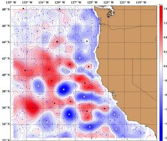
Mesoscale eddies (MEs) are energetic, swirling, time-dependent circulatory flows on a characteristic scale of around 100 km (see Fig. 1), which are observed almost ev-erywhere in satellite altimetry data of global sea surface height (Chelton et al., 2007, 2011). The total volume trans-port by drifting eddies is comparable in magnitude to that of the large-scale wind-driven and thermohaline circulations (Zhang et al., 2014); therefore, MEs play a crucial role in global material and heat transport and mixing of oceans. In spite of their importance, it is far from trivial to identify and characterize MEs from remote sensing data.

Figure 1.Visualization of the geostrophic flow field on a randomly chosen day (13 October 2013) from the data set over the US west coast by Risien and Strub (2016). Sea level anomalies (η) are color coded; blue stream lines indicate flow directions. The centers of cyclonic (yellow dots) and anticyclonic (black dots) eddies are determined by a standard algorithm (Chelton et al., 2011).

The original aim of our work was a detailed analysis of ki-netic energy budget of the oceanic surface flow field along the US west coast. At the evaluation of integrated kinetic energy and enstrophy (squared vorticity), we found a non-trivial strong temporal correlation between these quantities. Since the dominating flow features are obviously mesoscale eddies (Fig. 1), it is rather straightforward to formulate an ex-planation related to the description of individual ocean vor-tices. One of the basic models is the Gaussian geostrophic vortex exhibiting the attractive features of finite total energy and total enstrophy over an infinite domain, and a simple closed relationship between them. We demonstrate here that a single Gaussian super-vortex properly describes the empir-ical energy/enstrophy ratio over an extended region; further-more, the height and radius of such super-vortex are strongly related to the mean values over the same area obtained by classical vortex census.

2 Shielded Gaussian vortices

As for the shape of ocean MEs, the common picture is that they are close to Gaussian humps or troughs (Hopfinger and van Heijst, 1993; Chelton et al., 2011). A detailed fitting pro-cedure of about 5 million SLA profiles by Wang et al. (2015) revealed that around 50 % of MEs are indeed Gaussian,

an-other ∼40 % are Gaussian over a sloping background or merger of two close Gaussian eddies, and the rest have a quadratic core resembling Rankine vortices.

An isolated Gaussian circular eddy in geostrophic equilib-rium (where the hydrostatic pressure gradient force is bal-anced by the local Coriolis force) can be characterized by the following radial profiles of heightη, tangential velocityv and vertical vorticityξ (in cylindrical coordinates):

η(r)=η0exp

− r

2

2R2

, (1)

v(r)= −η0g

f R2rexp

− r

2

2R2

, (2)

ξ(r)= η0g

f R2

_r2

R2−2

exp

− r

2

2R2

. (3)

Here,η0andRare the height and size parameters for the vor-tex, respectively,gis the gravitational acceleration, andf=

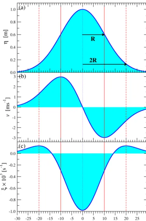
2sin(ϕ)is the local Coriolis parameter at latitudeϕ with =7.292×10−5s−1for the Earth. The label “shielded” in the title of this section refers to the core of such a vortex being surrounded by a ring of opposite vorticity (Tóth and Jánosi, 2015); see Fig. 2c.

Figure 2.Characteristics of a shielded Gaussian geostrophic vor-tex with peak height η0=1 m and size parameterR=10 km at an approximate location of 45◦N latitude (Coriolis parameterf= 10−4s−1).(a)Amplitude (see Eq. 1),(b)tangential velocity (see Eq. 2) and(c)vertical vorticity (see Eq. 3) as a function of radial distancer. Note thatRis the radial distance of maximum tangen-tial velocity (vertical red line), and 2R is the distance of maximal vorticity in the shielding ring (dashed vertical red line). The “visual” radius based on closed contours of zero height anomaly is around 2.5–3R.

the two-dimensional (2-D) barotropic Navier–Stokes equa-tions in a co-rotating frame of reference (Bracco et al., 2004). In the absence of dissipative processes, such a model con-serves the total kinetic energyRRKE=1

2

RR

v2dAand total enstrophy RR

Z=1

2

RR

ξ2dA. An appealing property of an isolated Gaussian vortex is that its total kinetic energy and enstrophy are finite over an infinite domain of integration:

IKE=1

2 ∞ Z

0

2π rv2(r)dr=g

2_{π η}2 0

2f2 , (4)

3 Data analysis

Simple visual inspection of a reconstructed geostrophic flow field (Fig. 1) reveals that MEs are indeed the dominating fea-tures. The area shown in Fig. 1 is an extremely well-studied region of the California Current System (CCS) both by ob-servations and calibrated high-resolution numerical simula-tions (Kelly et al., 1998; Strub and James, 2000; March-esiello et al., 2003; Castelao et al., 2006; Stegmann and Schwing, 2007; Capet et al., 2008a, b; Checkley and Barth, 2009; Matthews and Emery, 2009; Kurian et al., 2011; Mole-maker et al., 2015; Yuan and Castelao, 2017). Openly avail-able data compiled by Risien and Strub (2016) comprise a set of fields of sea level anomalies by combining gridded daily altimeter fields with coastal tide gauge data (Saraceno et al., 2008). The geographic area covers 32.0–48.5◦N (latitude) and 135.0–111.25◦W (longitude) with a spatial resolution of 0.25◦×0.25◦. Daily mean geostrophic velocity fields are produced for the period 1 January 1993–31 December 2014 (8035 d). The primary validation compares geostrophic ve-locities calculated from the SLA values and veve-locities mea-sured at four mooring sites in the test region (Risien and Strub, 2016).

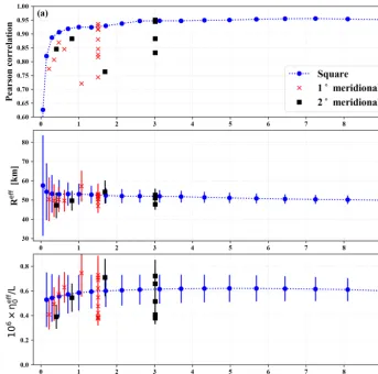
Figure 3 illustrates the total enstrophy (squared vorticity) and total kinetic energy (sum of squared velocity compo-nents) integrated over the offshore region (see the dashed frame in Fig. 4) for each day of the record. The correlation is strikingly strong, and it is not trivial. When the shore region is included, much larger differences appear, especially when the area of integration is restricted to a narrow band along the shoreline. Figure 5a clearly demonstrates that large correla-tion coefficients require large enough areas of integracorrela-tion; a value of 0.95 is reached aroundA=2.7×105km2 (∼202 grid cells or 5◦×5◦). Nevertheless, the geometry of the area must not be a square. The red and black symbols in Fig. 5a belong to meridional stripes of width of 1 and 2◦_longitudes (smaller areas are stripes eastward from 125.0◦_{W where the} meridional length is restricted by the land). Their apparent scatter, however, is not random; the correlation coefficients in equal areas of integration (symbols lined up vertically in Fig. 5a) systematically increase with the distance from the shoreline.

Figure 3. (a)The 10 years of daily values for total enstrophy (red) and rescaled total kinetic energy (blue) integrated over the offshore region (westward from 125.0◦W longitude; see Fig. 4) and(b)correlation plot of the two quantities. The rescaling factor for the kinetic energy integral is 7.97×10−10(see text).

Figure 4.Visualization of the geostrophic flow field on the same day as in Fig. 1 (13 October 2013) from the data set over the US west coast by Risien and Strub (2016). Empirical vertical vorticity (ξ) is color coded; blue stream lines indicate flow directions. The color mesh illustrates the spatial resolution well. The heavy dashed frame indicates the offshore region, where the integrated quantities in Fig. 3 are determined, and the yellow circle demonstrates the size of the hypothetical “super-vortex” related to mean vortex statistics on the given day over the offshore region (see text). Black squares illustrate the first 15 growing integration frames centered at the location 40.125◦N, 130.125◦W (see Fig. 5).

effective size parameter of a hypothetical Gaussian super-vortex as Reff=

q

2RRKE/RRZ. Results for the temporal mean values of this quantity are shown in Fig. 5b. Note that the obtained Reff≈50 km scale belongs to the 1σ width of a Gaussian profile given by Eq. (1). A visual contour of the super-vortex on a SLA map would have a radius closer to

∼2.5–3Reff≈125–150 km (see Figs. 2a and 4).

As for the height parameter of the super-vortex, Eq. (4) is used for an estimate ofηeff₀ shown in Fig. 5c. Since it is obtained from the total kinetic energy integrated over var-ious areas A, an appropriate comparison requires a proper normalization. A practical choice somewhat correcting shape differences is the characteristic length scaleL=

√

conse-Figure 5. (a)Pearson correlation coefficient for the total kinetic energy and enstrophy as a function of the area of integration. Blue circles indicate growing correlations for square-shaped areas around a central grid cell in the offshore region (40.125◦N, 130.125◦W); see Fig. 4. Red crosses (black squares) denote correlation coefficients for meridional stripes of width of 1◦(2◦) longitude.(b)Fitted mean scale param-eterRefffor a super-vortex determined from the ratio of integrated kinetic energy and enstrophy (in kilometers). Notations are the same as in panel(a).(c)Fitted mean height parameterηeff₀ normalized by the square root of the area of integrationL(and rescaled for the sake of convenience) for a super-vortex determined from the integrated kinetic energy; see Eq. (4). Notations are the same as in panel(a).

quence of the marked annual oscillations shown in Fig. 3a. These oscillations are canceled when the ratio of strongly correlated kinetic energy and enstrophy is considered. Simi-larly to the correlation coefficients in Fig. 5a, the fitted height values ofη₀efffor the meridional stripes (red crosses and black squares) exhibit systematic changes with the distance from the shoreline, as discussed below.

4 Eddy census

The super-vortex fit makes only sense when the parameters have some relationship with the existing MEs. In order to make such a comparison, we implemented the eddy census procedure of Chelton et al. (2011) based on closed SLA con-tour searches. The methodology is described in Chelton et al. (2011) and Oliver et al. (2015); here, we emphasize three par-ticular details. (i) The SLA fields in the data bank (Risien and

Figure 6. (a)Normalized eddy-scale distributions obtained by in-dividual eddy census with the closed contour SLA method (Chel-ton et al., 2011) at three different level spacing parameters1l; see legends. Vertical dotted lines indicate the mean values of the his-tograms. Black curve denotes the normalized histogram ofReff pa-rameter of the super-vortex. The logarithm of frequencies is scaled on the vertical scale.(b)Normalized eddy height distributions ob-tained by individual vortex census as in panel(a). The inset shows the histogram for the height parameter of the super-vortex fitηeff₀ in meters. Both the eddy census and super-vortex fit were performed over the offshore region (westward from 125.0◦W longitude; see Fig. 4).

identify smaller eddies in a larger number. The oscillations at smaller eddy scales are due to the discretization error; the area of an eddy is composed of an integer number of grid cells. It is clear that the fitted super-vortex parameter Reff fluctuates around the mean values of eddy-scale histograms (black curve in Fig. 6a). We reiterate here thatReffis an 1σ radius of a Gaussian vortex, whileSis closer to a “real” vi-sual radius based on a closed contour estimate of zero height anomaly. As for the super-vortex heightη₀eff, Fig. 6b illus-trates that it is much larger than the height of individual ed-dies, as expected, because it is related to the total kinetic en-ergy over the test area (the offshore region, in the particular case). For this reason, we compare the square of eddy ampli-tudes in what follows.

The significant advantage of using the super-vortex pic-ture emerges when the fits are performed over subregions of the test area. We have shown already results for meridional

Figure 7. (a)Fitted mean super-vortex radiusReff and mean eddy scalehSifrom eddy census, determined in meridional bands and plotted as a function of mean distance from the shore.(b)Square of fitted mean super-vortex height

ηeff₀

2

and the sum of squares

of all individual eddy heightsP

η2₀normalized by the area of in-tegration or eddy censusA.(c)Estimated westward drift velocities by evaluating the cross-correlation function (Eq. 6) and from vortex tracking of MEs living at least 60 d.

ratio of around 2 arises in each meridional stripe; that is, the long-term mean value of kinetic energy for individually identified eddies is∼50 % of the total kinetic energy in the test region. Interestingly, Amores et al. (2018) reported on a partition ratio between 1 and 5 fluctuating strongly in time; however, they note that the total kinetic energy obtained for satellite altimetry accounts only for half of the real value. The tendency of initial growth up to∼150 km (see Fig. 7b) might be related to the fact that eddies are generated mostly along the shore, and later they slowly decay during the drift in open water.

A well-known characteristic of eddy trajectories is the strong tendency for purely westward propagation (Cushman-Roisin et al., 1990; Chelton et al., 2007, 2011; Kurian et al., 2011). Chelton et al. (2007) found globally that only about 0.25 % of the eddies have mean drift directions that devi-ated by more than 10◦ from pure zonal; however, Kurian et al. (2011) and Stegmann and Schwing (2007) obtained stronger dispersion in the CCS study area. Together with the traditional eddy-tracking algorithm, we used our approach to evaluate the cross-correlations of total kinetic energyI (t )=

1 2

RR

v2dAbetween neighboring meridional bands of width of a single grid cell (0.25◦):

X(τ )=h[I(t )i−Ii][I(t±τ )i−1−Ii−1]i

σiσi−1

, (6)

where the time lagτ represents a temporal shift between the two time series byτ days, overbar denotes temporal mean, and σ is the standard deviation in the given band. Indeed, we find clear maxima at nonzero time lags (actual values are between 5 and 8 d) indicating that total kinetic energy and enstrophy are mostly advected in the offshore region; pro-duction or loss is almost negligible (considering geostrophic flow). The time lag and distance of neighboring bands permit an easy estimate of westward drift velocities; the results are shown in Fig. 7c. Drift velocity values in the literature are of the same order of magnitude (Stegmann and Schwing, 2007; Kurian et al., 2011; Chelton et al., 2007, 2011), similarly to our test. As for a direct validation, all individual eddy tracks are evaluated which had longer lifetime than 60 d (432 cy-clonic and 422 anticycy-clonic MEs are identified). The cut at 60 d is somewhat arbitrary; however, we think that the detec-tion error from both the limited spatial and temporal resolu-tions is larger for short living vortices (note that the typical

5 Conclusions

We proposed a simple description of geostrophic ocean sur-face flow fields by exploiting the following results. Firstly, a shielded Gaussian vortex has a finite total kinetic energy and finite total enstrophy; the ratio of them is proportional to the square of the radius of the vortex. Secondly, these two quan-tities determined from empirical velocity data are strongly correlated, and their ratio correlates with the mean eddy size obtained from traditional eddy census. Thirdly, the fitted am-plitude parameter is strongly related to the sum of all squared eddy amplitudes. While this description cannot replace tradi-tional eddy census algorithms, it is certainly able to extract coarse-grained eddy statistics in order to follow temporal and regional changes of eddy activity.

Data availability. The ocean flow field data are acces-sible at https://doi.org/10.1038/sdata.2016.13 (Risien and Strub, 2016). A direct link to the data download page is https://doi.org/10.7267/N9639MWJ.

Author contributions. IMJ designed the research; IMJ and MV performed the research; GT and JACG contributed new numeri-cal/analytical tools; IMJ and GT analyzed data; and IMJ, MV and JACG wrote the paper.

Competing interests. The authors declare no conflict of interest.

Acknowledgements. This work was supported by the Max-Planck Institute for the Physics of Complex Systems in the framework of an Advanced Study Group on “Forecasting with Lyapunov Vectors”. Jason A. C. Gallas was supported by CNPq, Brazil.

Financial support. This research has been supported by the Hungarian National Research, Development and Innovation Office (grant nos. FK-125024 and K-125171).

Review statement. This paper was edited by Eric J. M. Delhez and reviewed by two anonymous referees.

References

Amores, A., Jordà, G., Arsouze, T., and Le Sommer, J.: Up to what extent can we characterize ocean eddies using present-day grid-ded altimetric products?, J. Geophys. Res.-Oceans, 123, 7220– 7236, https://doi.org/10.1029/2018JC014140, 2018.

Beron-Vera, F. J., Hadjighasem, A., Xia, Q., Olascoaga, M. J., and Haller, G.: Coherent Lagrangian swirls among submesoscale motions, P. Natl. Acad. Sci. USA, 1–6, https://doi.org/10.1073/pnas.1701392115, 2018.

Bracco, A., von Hardenberg, J., Provenzale, A., Weiss, J. B., and McWilliams, J. C.: Dispersion and mixing in quasi-geostrophic turbulence, Phys. Rev. Lett., 92, 084501, https://doi.org/10.1103/PhysRevLett.92.084501, 2004.

Capet, X., McWilliams, J. C., Molemaker, M. J., and Shchep-etkin, A. F.: Mesoscale to submesoscale transition in the California Current System. Part I: Flow structure, eddy flux, and observational tests, J. Phys. Oceanogr., 38, 29–43, https://doi.org/10.1175/2007JPO3671.1, 2008a.

Capet, X., McWilliams, J. C., Molemaker, M. J., and Shchepetkin, A. F.: Mesoscale to submesoscale transition in the California Current System. Part II: Frontal processes, J. Phys. Oceanogr., 38, 44–64, https://doi.org/10.1175/2007JPO3672.1, 2008b. Castelao, R. M., Mavor, T. P., Barth, J. A., and Breaker, L. C.: Sea

surface temperature fronts in the California Current System from geostationary satellite observations, J. Geophys. Res.-Oceans, 111, C09026, https://doi.org/10.1029/2006JC003541, 2006. Checkley, D. M. and Barth, J. A.: Patterns and processes in

the California Current System, Progr. Oceanogr., 83, 49–64, https://doi.org/10.1016/j.pocean.2009.07.028, 2009.

Chelton, D. B., Schlax, M. G., Samelson, R. M., and de Szoeke, R. A.: Global observations of large oceanic eddies, Geophys. Res. Lett., 34, L15606, https://doi.org/10.1029/2007GL030812, 2007.

Chelton, D. B., Schlax, M. G., and Samelson, R. M.: Global ob-servations of nonlinear mesoscale eddies, Progr. Oceanogr., 91, 167–216, https://doi.org/10.1016/j.pocean.2011.01.002, 2011. Cushman-Roisin, B., Tang, B., and Chassignet, E. P.:

Westward motion of mesoscale eddies, J. Phys. Oceanogr., 20, 758–768, https://doi.org/10.1175/1520-0485(1990)020<0758:WMOME>2.0.CO;2, 1990.

Escudier, R., Renault, L., Pascual, A., Brasseur, P., Chel-ton, D., and Beuvier, J.: Eddy properties in the Western Mediterranean Sea from satellite altimetry and a numeri-cal simulation, J. Geophys. Res.-Oceans, 121, 3990–4006, https://doi.org/10.1002/2015JC011371, 2016.

Hadjighasem, A., Farazmand, M., Blazevski, D., Froyland, G., and Haller, G.: A critical comparison of Lagrangian meth-ods for coherent structure detection, Chaos, 27, 053104, https://doi.org/10.1063/1.4982720, 2017.

Haller, G.: Lagrangian coherent structures, Annu. Rev. Fluid Mech., 47, 137—162, https://doi.org/10.1146/annurev-fluid-010313-141322, 2015.

Haller, G., Karrasch, D., and Kogelbauer, F.: Material barriers to diffusive and stochastic transport, P. Natl. Acad. Sci. USA, 115, 9074–9079, https://doi.org/10.1073/pnas.1720177115, 2018. Hopfinger, E. J. and van Heijst, G. J. F.: Vortices in

rotating fluids, Annu. Rev. Fluid Mech., 25, 241–289, https://doi.org/10.1146/annurev.fl.25.010193.001325, 1993. Kelly, K. A., Beardsley, R. C., Brink, R. L. K. H., Paduan, J. D.,

and Chereskin, T. K.: Variability of the near-surface eddy ki-netic energy in the California Current based on altimetric, drifter, and moored current data, J. Geophys. Res., 103, 13067–13083, https://doi.org/10.1029/97JC03760, 1998.

Kurian, J., Colas, F., Capet, X., McWilliams, J. C., and Chelton, D. B.: Eddy properties in the Califor-nia Current System, J. Geophys. Res., 116, C08027, https://doi.org/10.1029/2010JC006895, 2011.

Li, Q.-Y., Sun, L., and Lin, S.-F.: GEM: a dynamic tracking model for mesoscale eddies in the ocean, Ocean Sci., 12, 1249–1267, https://doi.org/10.5194/os-12-1249-2016, 2016.

Li, Q.-Y., Sun, L., and Xu, C.: The lateral eddy viscosity derived from the decay of oceanic mesoscale eddies, Open J. Marine Sci., 8, 152–172, https://doi.org/10.4236/ojms.2018.81008, 2018. Marchesiello, P., McWilliams, J. C., and Shchepetkin, A.:

Equilib-rium structure and dynamics of the California Current System, J. Phys. Oceanogr., 33, 753–783, https://doi.org/10.1175/1520-0485(2003)33<753:ESADOT>2.0.CO;2, 2003.

Mason, E., Pascual, A., and McWilliams, J. C.: A new sea surface height–based code for oceanic mesoscale eddy tracking, J. Atmos. Oceanic Technol., 31, 1181–1188, https://doi.org/10.1175/JTECH-D-14-00019.1, 2014.

Matthews, D. K. and Emery, W. J.: Velocity observations of the Cal-ifornia Current derived from satellite imagery, J. Geophys. Res., 114, C08001, https://doi.org/10.1029/2008JC005029, 2009. Molemaker, M. J., McWilliams, J. C., and Dewar, W. K.:

Subme-soscale instability and generation of meSubme-soscale anticyclones near a separation of the California Undercurrent, J. Phys. Oceanogr., 45, 613–629, https://doi.org/10.1175/JPO-D-13-0225.1, 2015. Nencioli, F., Dong, C., Dickey, T., Washburn, L., and McWilliams,

J. C.: A vector geometry–based eddy detection algorithm and its application to a high-resolution numerical model product and high-frequency radar surface velocities in the Southern California Bight, J. Atmos. Oceanic Technol., 27, 564–579, https://doi.org/10.1175/2009JTECHO725.1, 2010.

Oliver, E. C. J., O’Kane, T. J., and Holbrook, N. J.: Projected changes to Tasman Sea eddies in a future climate, J. Geophys. Res.-Oceans, 120, 7150–7165, https://doi.org/10.1002/2015JC010993, 2015.

Pessini, F., Olita, A., Cotroneo, Y., and Perilli, A.: Mesoscale eddies in the Algerian Basin: do they differ as a func-tion of their formafunc-tion site?, Ocean Science, 14, 669–688, https://doi.org/10.5194/os-14-669-2018, 2018.

Pnyushkov, A., Polyakov, I. V., Padman, L., and Nguyen, A. T.: Structure and dynamics of mesoscale eddies over the Laptev Sea continental slope in the Arctic Ocean, Ocean Sci., 14, 1329– 1347, https://doi.org/10.5194/os-14-1329-2018, 2018.

Risien, C. M. and Strub, P. T.: Blended sea level anomaly fields with enhanced coastal coverage along the U.S. West Coast, Sci. Data, 3, 160013, https://doi.org/10.1038/sdata.2016.13, 2016. Rubio, A., Blanke, B., Speich, S., Grima, N., and Roy, C.:

sys-tification algorithms for the quansys-tification and characterization of mesoscale eddies in the South Atlantic Ocean, Ocean Sci., 7, 317–334, https://doi.org/10.5194/os-7-317-2011, 2011. Stegmann, P. M. and Schwing, F.: Demographics of mesoscale

ed-dies in the California Current, Geophys. Res. Lett., 34, L14602, https://doi.org/10.1029/2007GL029504, 2007.

Strub, P. T. and James, C.: Altimeter-derived variability of surface velocities in the California Current System: 2. Seasonal circu-lation and eddy statistics, Deep-Sea Res. Pt. II, 47, 831–870, https://doi.org/10.1016/S0967-0645(99)00129-0, 2000.

rent Systems, J. Geophys. Res.-Oceans, 122, 4791–4801, https://doi.org/10.1002/2017JC012735, 2017.