Think Bayes
Bayesian Statistics Made Simple
Think Bayes
Bayesian Statistics Made Simple
Version 1.0.9
Allen B. Downey
Green Tea Press
Copyright © 2012 Allen B. Downey.
Green Tea Press 9 Washburn Ave Needham MA 02492
Permission is granted to copy, distribute, and/or modify this document under the terms of the Creative Commons Attribution-NonCommercial-ShareAlike 4.0 International License, which is available at http://creativecommons. org/licenses/by-nc-sa/4.0/.
The LATEX source for this book is available from http://greenteapress.com/
Preface
0.1 My theory, which is mine
The premise of this book, and the other books in the Think X series, is that if you know how to program, you can use that skill to learn other topics. Most books on Bayesian statistics use mathematical notation and present ideas in terms of mathematical concepts like calculus. This book uses Python code instead of math, and discrete approximations instead of continuous math-ematics. As a result, what would be an integral in a math book becomes a summation, and most operations on probability distributions are simple loops. I think this presentation is easier to understand, at least for people with pro-gramming skills. It is also more general, because when we make modeling decisions, we can choose the most appropriate model without worrying too much about whether the model lends itself to conventional analysis.
Also, it provides a smooth development path from simple examples to real-world problems. Chapter 3 is a good example. It starts with a simple example involving dice, one of the staples of basic probability. From there it proceeds in small steps to the locomotive problem, which I borrowed from Mosteller's Fifty Challenging Problems in Probability with Solutions, and from there to the German tank problem, a famously successful application of Bayesian methods during World War II.
0.2 Modeling and approximation
vi Chapter 0. Preface
For example, in Chapter 7, the motivating problem is to predict the winner of a hockey game. I model goal-scoring as a Poisson process, which implies that a goal is equally likely at any point in the game. That is not exactly true, but it is probably a good enough model for most purposes.
In Chapter 12 the motivating problem is interpreting SAT scores (the SAT is a standardized test used for college admissions in the United States). I start with a simple model that assumes that all SAT questions are equally dicult, but in fact the designers of the SAT deliberately include some questions that are relatively easy and some that are relatively hard. I present a second model that accounts for this aspect of the design, and show that it doesn't have a big eect on the results after all.
I think it is important to include modeling as an explicit part of problem solving because it reminds us to think about modeling errors (that is, errors due to simplications and assumptions of the model).
Many of the methods in this book are based on discrete distributions, which makes some people worry about numerical errors. But for real-world problems, numerical errors are almost always smaller than modeling errors.
Furthermore, the discrete approach often allows better modeling decisions, and I would rather have an approximate solution to a good model than an exact solution to a bad model.
On the other hand, continuous methods sometimes yield performance advantagesfor example by replacing a linear- or quadratic-time computa-tion with a constant-time solucomputa-tion.
So I recommend a general process with these steps:
1. While you are exploring a problem, start with simple models and im-plement them in code that is clear, readable, and demonstrably correct. Focus your attention on good modeling decisions, not optimization. 2. Once you have a simple model working, identify the biggest sources of
error. You might need to increase the number of values in a discrete approximation, or increase the number of iterations in a Monte Carlo simulation, or add details to the model.
0.3. Working with the code vii
One benet of this process is that Steps 1 and 2 tend to be fast, so you can explore several alternative models before investing heavily in any of them. Another benet is that if you get to Step 3, you will be starting with a reference implementation that is likely to be correct, which you can use for regression testing (that is, checking that the optimized code yields the same results, at least approximately).
0.3 Working with the code
The code and sound samples used in this book are available from https:// github.com/AllenDowney/ThinkBayes. Git is a version control system that allows you to keep track of the les that make up a project. A collection of les under Git's control is called a repository. GitHub is a hosting service that provides storage for Git repositories and a convenient web interface. The GitHub homepage for my repository provides several ways to work with the code:
You can create a copy of my repository on GitHub by pressing the Fork button. If you don't already have a GitHub account, you'll need to create one. After forking, you'll have your own repository on GitHub that you can use to keep track of code you write while working on this book. Then you can clone the repo, which means that you copy the les to your computer.
Or you could clone my repository. You don't need a GitHub account to do this, but you won't be able to write your changes back to GitHub. If you don't want to use Git at all, you can download the les in a Zip
le using the button in the lower-right corner of the GitHub page.
The code for the rst edition of the book works with Python 2. If you are using Python 3, you might want to use the updated code in https://github. com/AllenDowney/ThinkBayes2 instead.
I developed this book using Anaconda from Continuum Analytics, which is a free Python distribution that includes all the packages you'll need to run the code (and lots more). I found Anaconda easy to install. By default it does a user-level installation, not system-level, so you don't need administrative priv-ileges. You can download Anaconda from http://continuum.io/downloads.
viii Chapter 0. Preface
NumPy for basic numerical computation, http://www.numpy.org/; SciPy for scientic computation, http://www.scipy.org/;
matplotlib for visualization, http://matplotlib.org/.
Although these are commonly used packages, they are not included with all Python installations, and they can be hard to install in some environments. If you have trouble installing them, I recommend using Anaconda or one of the other Python distributions that include these packages.
Many of the examples in this book use classes and functions dened in thinkbayes.py. Some of them also use thinkplot.py, which provides wrap-pers for some of the functions in pyplot, which is part of matplotlib.
0.4 Code style
Experienced Python programmers will notice that the code in this book does not comply with PEP 8, which is the most common style guide for Python (http://www.python.org/dev/peps/pep-0008/).
Specically, PEP 8 calls for lowercase function names with underscores be-tween words, like_this. In this book and the accompanying code, function and method names begin with a capital letter and use camel case, LikeThis. I broke this rule because I developed some of the code while I was a Visiting Scientist at Google, so I followed the Google style guide, which deviates from PEP 8 in a few places. Once I got used to Google style, I found that I liked it. And at this point, it would be too much trouble to change.
Also on the topic of style, I write Bayes's theorem with an s after the apos-trophe, which is preferred in some style guides and deprecated in others. I don't have a strong preference. I had to choose one, and this is the one I chose.
And nally one typographical note: throughout the book, I use PMF and CDF for the mathematical concept of a probability mass function or cumulative distribution function, and Pmf and Cdf to refer to the Python objects I use to represent them.
0.5 Prerequisites
0.5. Prerequisites ix
you need a fair amount of background knowledge to get started with these modules, and I want to keep the prerequisites minimal. If you know Python and a little bit about probability, you are ready to start this book.
Chapter 1 is about probability and Bayes's theorem; it has no code. Chap-ter 2 introduces Pmf, a thinly disguised Python dictionary I use to represent a probability mass function (PMF). Then Chapter 3 introduces Suite, a kind of Pmf that provides a framework for doing Bayesian updates.
In some of the later chapters, I use analytic distributions including the Gaus-sian (normal) distribution, the exponential and Poisson distributions, and the beta distribution. In Chapter 15 I break out the less-common Dirichlet dis-tribution, but I explain it as I go along. If you are not familiar with these distributions, you can read about them on Wikipedia. You could also read the companion to this book, Think Stats, or an introductory statistics book (although I'm afraid most of them take a mathematical approach that is not particularly helpful for practical purposes).
Contributor List
If you have a suggestion or correction, please send email to [email protected]. If I make a change based on your feedback, I will add you to the contributor list (unless you ask to be omitted).
If you include at least part of the sentence the error appears in, that makes it easy for me to search. Page and section numbers are ne, too, but not as easy to work with. Thanks!
First, I have to acknowledge David MacKay's excellent book, Information Theory, Inference, and Learning Algorithms, which is where I rst came to understand Bayesian methods. With his permission, I use several problems from his book as examples.
This book also beneted from my interactions with Sanjoy Mahajan, especially in fall 2012, when I audited his class on Bayesian Inference at Olin College. I wrote parts of this book during project nights with the Boston Python User
Group, so I would like to thank them for their company and pizza. Olivier Yiptong sent several helpful suggestions.
Yuriy Pasichnyk found several errors.
x Chapter 0. Preface
Markus Dobler pointed out that drawing cookies from a bowl with replacement is an unrealistic scenario.
In spring 2013, students in my class, Computational Bayesian Statistics, made many helpful corrections and suggestions: Kai Austin, Claire Barnes, Kari Bender, Rachel Boy, Kat Mendoza, Arjun Iyer, Ben Kroop, Nathan Lintz, Kyle McConnaughay, Alec Radford, Brendan Ritter, and Evan Simpson. Greg Marra and Matt Aasted helped me clarify the discussion of The Price is
Right problem.
Marcus Ogren pointed out that the original statement of the locomotive prob-lem was ambiguous.
Jasmine Kwityn and Dan Fauxsmith at O'Reilly Media proofread the book and found many opportunities for improvement.
Linda Pescatore found a typo and made some helpful suggestions. Tomasz Mi¡sko sent many excellent corrections and suggestions.
Contents
Preface v
0.1 My theory, which is mine . . . v
0.2 Modeling and approximation . . . v
0.3 Working with the code . . . vii
0.4 Code style . . . viii
0.5 Prerequisites . . . viii
1 Bayes's Theorem 1 1.1 Conditional probability . . . 1
1.2 Conjoint probability . . . 2
1.3 The cookie problem . . . 3
1.4 Bayes's theorem . . . 3
1.5 The diachronic interpretation . . . 5
1.6 The M&M problem . . . 6
1.7 The Monty Hall problem . . . 8
1.8 Discussion . . . 10
2 Computational Statistics 11 2.1 Distributions . . . 11
2.2 The cookie problem . . . 12
xii Contents
2.4 The Monty Hall problem . . . 15
2.5 Encapsulating the framework . . . 16
2.6 The M&M problem . . . 17
2.7 Discussion . . . 18
2.8 Exercises . . . 18
3 Estimation 21 3.1 The dice problem . . . 21
3.2 The locomotive problem . . . 22
3.3 What about that prior? . . . 25
3.4 An alternative prior . . . 25
3.5 Credible intervals . . . 27
3.6 Cumulative distribution functions . . . 28
3.7 The German tank problem . . . 29
3.8 Discussion . . . 29
3.9 Exercises . . . 30
4 More Estimation 33 4.1 The Euro problem . . . 33
4.2 Summarizing the posterior . . . 35
4.3 Swamping the priors . . . 37
4.4 Optimization . . . 37
4.5 The beta distribution . . . 39
4.6 Discussion . . . 40
Contents xiii
5 Odds and Addends 43
5.1 Odds . . . 43
5.2 The odds form of Bayes's theorem . . . 44
5.3 Oliver's blood . . . 45
5.4 Addends . . . 46
5.5 Maxima . . . 50
5.6 Mixtures . . . 52
5.7 Discussion . . . 54
6 Decision Analysis 55 6.1 The Price is Right problem . . . 55
6.2 The prior . . . 56
6.3 Probability density functions . . . 57
6.4 Representing PDFs . . . 57
6.5 Modeling the contestants . . . 60
6.6 Likelihood . . . 62
6.7 Update . . . 63
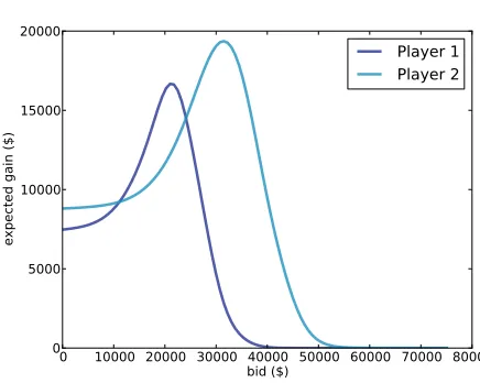
6.8 Optimal bidding . . . 64
6.9 Discussion . . . 67
7 Prediction 69 7.1 The Boston Bruins problem . . . 69
7.2 Poisson processes . . . 70
7.3 The posteriors . . . 71
7.4 The distribution of goals . . . 72
7.5 The probability of winning . . . 74
7.6 Sudden death . . . 75
7.7 Discussion . . . 76
xiv Contents
8 Observer Bias 79
8.1 The Red Line problem . . . 79
8.2 The model . . . 79
8.3 Wait times . . . 81
8.4 Predicting wait times . . . 84
8.5 Estimating the arrival rate . . . 86
8.6 Incorporating uncertainty . . . 89
8.7 Decision analysis . . . 90
8.8 Discussion . . . 92
8.9 Exercises . . . 93
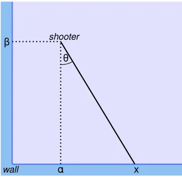
9 Two Dimensions 95 9.1 Paintball . . . 95
9.2 The suite . . . 96
9.3 Trigonometry . . . 97
9.4 Likelihood . . . 99
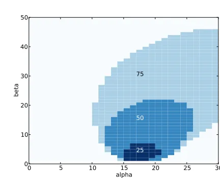
9.5 Joint distributions . . . 100
9.6 Conditional distributions . . . 100
9.7 Credible intervals . . . 102
9.8 Discussion . . . 104
9.9 Exercises . . . 105
10 Approximate Bayesian Computation 107 10.1 The Variability Hypothesis . . . 107
10.2 Mean and standard deviation . . . 108
10.3 Update . . . 110
10.4 The posterior distribution of CV . . . 111
Contents xv
10.6 Log-likelihood . . . 113
10.7 A little optimization . . . 114
10.8 ABC . . . 116
10.9 Robust estimation . . . 117
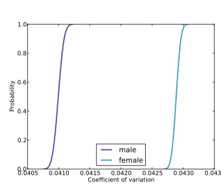
10.10 Who is more variable? . . . 120
10.11 Discussion . . . 121
10.12 Exercises . . . 122
11 Hypothesis Testing 123 11.1 Back to the Euro problem . . . 123
11.2 Making a fair comparison . . . 124
11.3 The triangle prior . . . 126
11.4 Discussion . . . 127
11.5 Exercises . . . 127
12 Evidence 129 12.1 Interpreting SAT scores . . . 129
12.2 The scale . . . 130
12.3 The prior . . . 130
12.4 Posterior . . . 132
12.5 A better model . . . 134
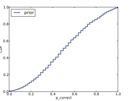
12.6 Calibration . . . 136
12.7 Posterior distribution of ecacy . . . 137
12.8 Predictive distribution . . . 139
xvi Contents
13 Simulation 143
13.1 The Kidney Tumor problem . . . 143
13.2 A simple model . . . 144
13.3 A more general model . . . 146
13.4 Implementation . . . 148
13.5 Caching the joint distribution . . . 149
13.6 Conditional distributions . . . 150
13.7 Serial Correlation . . . 151
13.8 Discussion . . . 155
14 A Hierarchical Model 157 14.1 The Geiger counter problem . . . 157
14.2 Start simple . . . 158
14.3 Make it hierarchical . . . 159
14.4 A little optimization . . . 160
14.5 Extracting the posteriors . . . 161
14.6 Discussion . . . 162
14.7 Exercises . . . 163
15 Dealing with Dimensions 165 15.1 Belly button bacteria . . . 165
15.2 Lions and tigers and bears . . . 166
15.3 The hierarchical version . . . 168
15.4 Random sampling . . . 170
15.5 Optimization . . . 172
15.6 Collapsing the hierarchy . . . 173
15.7 One more problem . . . 175
Contents xvii
15.9 The belly button data . . . 178
15.10 Predictive distributions . . . 181
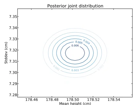
15.11 Joint posterior . . . 185
15.12 Coverage . . . 186
Chapter 1
Bayes's Theorem
1.1 Conditional probability
The fundamental idea behind all Bayesian statistics is Bayes's theorem, which is surprisingly easy to derive, provided that you understand conditional proba-bility. So we'll start with probability, then conditional probability, then Bayes's theorem, and on to Bayesian statistics.
A probability is a number between 0 and 1 (including both) that represents a degree of belief in a fact or prediction. The value 1 represents certainty that a fact is true, or that a prediction will come true. The value 0 represents certainty that the fact is false.
Intermediate values represent degrees of certainty. The value 0.5, often written as 50%, means that a predicted outcome is as likely to happen as not. For example, the probability that a tossed coin lands face up is very close to 50%.
A conditional probability is a probability based on some background informa-tion. For example, I want to know the probability that I will have a heart at-tack in the next year. According to the CDC, Every year about 785,000 Amer-icans have a rst coronary attack. (http://www.cdc.gov/heartdisease/ facts.htm)
2 Chapter 1. Bayes's Theorem
I am male, 45 years old, and I have borderline high cholesterol. Those factors increase my chances. However, I have low blood pressure and I don't smoke, and those factors decrease my chances.
Plugging everything into the online calculator at http://cvdrisk.nhlbi. nih.gov/calculator.asp, I nd that my risk of a heart attack in the next year is about 0.2%, less than the national average. That value is a condi-tional probability, because it is based on a number of factors that make up my condition.
The usual notation for conditional probability isp(A|B), which is the
proba-bility of A given that B is true. In this example, A represents the prediction
that I will have a heart attack in the next year, and B is the set of conditions
I listed.
1.2 Conjoint probability
Conjoint probability is a fancy way to say the probability that two things
are true. I write p(A and B) to mean the probability that A and B are both
true.
If you learned about probability in the context of coin tosses and dice, you might have learned the following formula:
p(A and B) = p(A) p(B) WARNING: not always true
For example, if I toss two coins, andAmeans the rst coin lands face up, and
B means the second coin lands face up, then p(A) = p(B) = 0.5, and sure
enough, p(A and B) = p(A) p(B) = 0.25.
But this formula only works because in this case A and B are independent;
that is, knowing the outcome of the rst event does not change the probability of the second. Or, more formally,p(B|A) =p(B).
Here is a dierent example where the events are not independent. Suppose
that A means that it rains today and B means that it rains tomorrow. If
I know that it rained today, it is more likely that it will rain tomorrow, so
p(B|A)>p(B).
In general, the probability of a conjunction is
p(A and B) = p(A) p(B|A)
for any A and B. So if the chance of rain on any given day is 0.5, the chance
1.3. The cookie problem 3
1.3 The cookie problem
We'll get to Bayes's theorem soon, but I want to motivate it with an example
called the cookie problem.1 Suppose there are two bowls of cookies. Bowl 1
contains 30 vanilla cookies and 10 chocolate cookies. Bowl 2 contains 20 of each.
Now suppose you choose one of the bowls at random and, without looking, select a cookie at random. The cookie is vanilla. What is the probability that it came from Bowl 1?
This is a conditional probability; we want p(Bowl 1|vanilla), but it is not
obvious how to compute it. If I asked a dierent questionthe probability of a vanilla cookie given Bowl 1it would be easy:
p(vanilla|Bowl 1) = 3/4
Sadly, p(A|B) is not the same as p(B|A), but there is a way to get from one
to the other: Bayes's theorem.
1.4 Bayes's theorem
At this point we have everything we need to derive Bayes's theorem. We'll start with the observation that conjunction is commutative; that is
p(A and B) = p(B and A)
for any events A and B.
Next, we write the probability of a conjunction:
p(A and B) = p(A) p(B|A)
Since we have not said anything about what A and B mean, they are
inter-changeable. Interchanging them yields
p(B and A) = p(B) p(A|B)
That's all we need. Pulling those pieces together, we get
p(B) p(A|B) = p(A) p(B|A)
1Based on an example from http://en.wikipedia.org/wiki/Bayes'_theorem that is
4 Chapter 1. Bayes's Theorem
Which means there are two ways to compute the conjunction. If you have
p(A), you multiply by the conditional probability p(B|A). Or you can do it
the other way around; if you knowp(B), you multiply by p(A|B). Either way
you should get the same thing.
Finally we can divide through byp(B):
p(A|B) = p(A) p(B|A) p(B)
And that's Bayes's theorem! It might not look like much, but it turns out to be surprisingly powerful.
For example, we can use it to solve the cookie problem. I'll write B1 for the
hypothesis that the cookie came from Bowl 1 and V for the vanilla cookie.
Plugging in Bayes's theorem we get
p(B1|V) =
p(B1) p(V|B1) p(V)
The term on the left is what we want: the probability of Bowl 1, given that we chose a vanilla cookie. The terms on the right are:
p(B1): This is the probability that we chose Bowl 1, unconditioned by
what kind of cookie we got. Since the problem says we chose a bowl at random, we can assume p(B1) = 1/2.
p(V|B1): This is the probability of getting a vanilla cookie from Bowl 1,
which is 3/4.
p(V): This is the probability of drawing a vanilla cookie from either
bowl. Since we had an equal chance of choosing either bowl and the bowls contain the same number of cookies, we had the same chance of choosing any cookie. Between the two bowls there are 50 vanilla and 30 chocolate cookies, so p(V) = 5/8.
Putting it together, we have
p(B1|V) = (1/2) (3/4) 5/8
1.5. The diachronic interpretation 5
This example demonstrates one use of Bayes's theorem: it provides a strategy to get from p(B|A) top(A|B). This strategy is useful in cases, like the cookie
problem, where it is easier to compute the terms on the right side of Bayes's theorem than the term on the left.
1.5 The diachronic interpretation
There is another way to think of Bayes's theorem: it gives us a way to update the probability of a hypothesis, H, in light of some body of data, D.
This way of thinking about Bayes's theorem is called the diachronic inter-pretation. Diachronic means that something is happening over time; in this case the probability of the hypotheses changes, over time, as we see new data.
Rewriting Bayes's theorem with H and D yields:
p(H|D) = p(H) p(D|H) p(D)
In this interpretation, each term has a name:
p(H) is the probability of the hypothesis before we see the data, called
the prior probability, or just prior.
p(H|D) is what we want to compute, the probability of the hypothesis
after we see the data, called the posterior.
p(D|H) is the probability of the data under the hypothesis, called the
likelihood.
p(D) is the probability of the data under any hypothesis, called the
normalizing constant.
Sometimes we can compute the prior based on background information. For example, the cookie problem species that we choose a bowl at random with equal probability.
In other cases the prior is subjective; that is, reasonable people might dis-agree, either because they use dierent background information or because they interpret the same information dierently.
6 Chapter 1. Bayes's Theorem
The normalizing constant can be tricky. It is supposed to be the probability of seeing the data under any hypothesis at all, but in the most general case it is hard to nail down what that means.
Most often we simplify things by specifying a set of hypotheses that are
Mutually exclusive: At most one hypothesis in the set can be true, and
Collectively exhaustive: There are no other possibilities; at least one of the hypotheses has to be true.
I use the word suite for a set of hypotheses that has these properties.
In the cookie problem, there are only two hypothesesthe cookie came from Bowl 1 or Bowl 2and they are mutually exclusive and collectively exhaustive.
In that case we can compute p(D) using the law of total probability, which
says that if there are two exclusive ways that something might happen, you can add up the probabilities like this:
p(D) = p(B1) p(D|B1) + p(B2) p(D|B2)
Plugging in the values from the cookie problem, we have
p(D) = (1/2) (3/4) + (1/2) (1/2) = 5/8
which is what we computed earlier by mentally combining the two bowls.
1.6 The M&M problem
M&M's are small candy-coated chocolates that come in a variety of colors. Mars, Inc., which makes M&M's, changes the mixture of colors from time to time.
In 1995, they introduced blue M&M's. Before then, the color mix in a bag of plain M&M's was 30% Brown, 20% Yellow, 20% Red, 10% Green, 10% Orange, 10% Tan. Afterward it was 24% Blue , 20% Green, 16% Orange, 14% Yellow, 13% Red, 13% Brown.
1.6. The M&M problem 7
This problem is similar to the cookie problem, with the twist that I draw one sample from each bowl/bag. This problem also gives me a chance to demonstrate the table method, which is useful for solving problems like this on paper. In the next chapter we will solve them computationally.
The rst step is to enumerate the hypotheses. The bag the yellow M&M came from I'll call Bag 1; I'll call the other Bag 2. So the hypotheses are:
A: Bag 1 is from 1994, which implies that Bag 2 is from 1996.
B: Bag 1 is from 1996 and Bag 2 from 1994.
Now we construct a table with a row for each hypothesis and a column for each term in Bayes's theorem:
Prior Likelihood Posterior
p(H) p(D|H) p(H) p(D|H) p(H|D)
A 1/2 (20)(20) 200 20/27
B 1/2 (14)(10) 70 7/27
The rst column has the priors. Based on the statement of the problem, it is
reasonable to choose p(A) = p(B) = 1/2.
The second column has the likelihoods, which follow from the information
in the problem. For example, if A is true, the yellow M&M came from the
1994 bag with probability 20%, and the green came from the 1996 bag with probability 20%. If B is true, the yellow M&M came from the 1996 bag with
probability 14%, and the green came from the 1994 bag with probability 10%. Because the selections are independent, we get the conjoint probability by multiplying.
The third column is just the product of the previous two. The sum of this col-umn, 270, is the normalizing constant. To get the last colcol-umn, which contains the posteriors, we divide the third column by the normalizing constant. That's it. Simple, right?
Well, you might be bothered by one detail. I write p(D|H) in terms of
per-centages, not probabilities, which means it is o by a factor of 10,000. But that cancels out when we divide through by the normalizing constant, so it doesn't aect the result.
8 Chapter 1. Bayes's Theorem
1.7 The Monty Hall problem
The Monty Hall problem might be the most contentious question in the history of probability. The scenario is simple, but the correct answer is so counter-intuitive that many people just can't accept it, and many smart people have embarrassed themselves not just by getting it wrong but by arguing the wrong side, aggressively, in public.
Monty Hall was the original host of the game show Let's Make a Deal. The Monty Hall problem is based on one of the regular games on the show. If you are on the show, here's what happens:
Monty shows you three closed doors and tells you that there is a prize behind each door: one prize is a car, the other two are less valuable prizes like peanut butter and fake nger nails. The prizes are arranged at random.
The object of the game is to guess which door has the car. If you guess right, you get to keep the car.
You pick a door, which we will call Door A. We'll call the other doors B and C.
Before opening the door you chose, Monty increases the suspense by opening either Door B or C, whichever does not have the car. (If the car is actually behind Door A, Monty can safely open B or C, so he chooses one at random.)
Then Monty oers you the option to stick with your original choice or switch to the one remaining unopened door.
The question is, should you stick or switch or does it make no dierence?
Most people have the strong intuition that it makes no dierence. There are two doors left, they reason, so the chance that the car is behind Door A is 50%.
But that is wrong. In fact, the chance of winning if you stick with Door A is only 1/3; if you switch, your chances are 2/3.
By applying Bayes's theorem, we can break this problem into simple pieces, and maybe convince ourselves that the correct answer is, in fact, correct.
To start, we should make a careful statement of the data. In this case D
1.7. The Monty Hall problem 9
Next we dene three hypotheses: A, B, and C represent the hypothesis that
the car is behind Door A, Door B, or Door C. Again, let's apply the table method:
Prior Likelihood Posterior
p(H) p(D|H) p(H) p(D|H) p(H|D)
A 1/3 1/2 1/6 1/3
B 1/3 0 0 0
C 1/3 1 1/3 2/3
Filling in the priors is easy because we are told that the prizes are arranged at random, which suggests that the car is equally likely to be behind any door. Figuring out the likelihoods takes some thought, but with reasonable care we can be condent that we have it right:
If the car is actually behind A, Monty could safely open Doors B or C. So the probability that he chooses B is 1/2. And since the car is actually behind A, the probability that the car is not behind B is 1.
If the car is actually behind B, Monty has to open door C, so the prob-ability that he opens door B is 0.
Finally, if the car is behind Door C, Monty opens B with probability 1 and nds no car there with probability 1.
Now the hard part is over; the rest is just arithmetic. The sum of the third column is 1/2. Dividing through yields p(A|D) = 1/3and p(C|D) = 2/3. So
you are better o switching.
There are many variations of the Monty Hall problem. One of the strengths of the Bayesian approach is that it generalizes to handle these variations. For example, suppose that Monty always chooses B if he can, and only chooses C if he has to (because the car is behind B). In that case the revised table is:
Prior Likelihood Posterior
p(H) p(D|H) p(H) p(D|H) p(H|D)
A 1/3 1 1/3 1/2
B 1/3 0 0 0
C 1/3 1 1/3 1/2
The only change is p(D|A). If the car is behind A, Monty can choose to open
B or C. But in this variation he always chooses B, so p(D|A) = 1.
As a result, the likelihoods are the same for A and C, and the posteriors are
10 Chapter 1. Bayes's Theorem
B reveals no information about the location of the car, so it doesn't matter whether the contestant sticks or switches.
On the other hand, if he had openedC, we would know p(B|D) = 1.
I included the Monty Hall problem in this chapter because I think it is fun, and because Bayes's theorem makes the complexity of the problem a little more manageable. But it is not a typical use of Bayes's theorem, so if you found it confusing, don't worry!
1.8 Discussion
For many problems involving conditional probability, Bayes's theorem
pro-vides a divide-and-conquer strategy. If p(A|B) is hard to compute, or hard
to measure experimentally, check whether it might be easier to compute the other terms in Bayes's theorem, p(B|A),p(A) and p(B).
Chapter 2
Computational Statistics
2.1 Distributions
In statistics a distribution is a set of values and their corresponding proba-bilities.
For example, if you roll a six-sided die, the set of possible values is the numbers 1 to 6, and the probability associated with each value is 1/6.
As another example, you might be interested in how many times each word appears in common English usage. You could build a distribution that includes each word and how many times it appears.
To represent a distribution in Python, you could use a dictionary that maps from each value to its probability. I have written a class called Pmf that uses a Python dictionary in exactly that way, and provides a number of useful methods. I called the class Pmf in reference to a probability mass function, which is a way to represent a distribution mathematically.
Pmf is dened in a Python module I wrote to accompany this book,
thinkbayes.py. You can download it from http://thinkbayes.com/
thinkbayes.py. For more information see Section 0.3. To use Pmf you can import it like this:
from thinkbayes import Pmf
The following code builds a Pmf to represent the distribution of outcomes for a six-sided die:
pmf = Pmf()
12 Chapter 2. Computational Statistics
Pmf creates an empty Pmf with no values. The Set method sets the probability associated with each value to1/6.
Here's another example that counts the number of times each word appears in a sequence:
pmf = Pmf()
for word in word_list: pmf.Incr(word, 1)
Incr increases the probability associated with each word by 1. If a word is not already in the Pmf, it is added.
I put probability in quotes because in this example, the probabilities are not normalized; that is, they do not add up to 1. So they are not true probabilities. But in this example the word counts are proportional to the probabilities. So after we count all the words, we can compute probabilities by dividing through by the total number of words. Pmf provides a method, Normalize, that does exactly that:
pmf.Normalize()
Once you have a Pmf object, you can ask for the probability associated with any value:
print pmf.Prob('the')
And that would print the frequency of the word the as a fraction of the words in the list.
Pmf uses a Python dictionary to store the values and their probabilities, so the values in the Pmf can be any hashable type. The probabilities can be any numerical type, but they are usually oating-point numbers (type float).
2.2 The cookie problem
In the context of Bayes's theorem, it is natural to use a Pmf to map from each
hypothesis to its probability. In the cookie problem, the hypotheses are B1
and B2. In Python, I represent them with strings:
pmf = Pmf()
pmf.Set('Bowl 1', 0.5) pmf.Set('Bowl 2', 0.5)
2.3. The Bayesian framework 13
To update the distribution based on new data (the vanilla cookie), we multiply each prior by the corresponding likelihood. The likelihood of drawing a vanilla cookie from Bowl 1 is 3/4. The likelihood for Bowl 2 is 1/2.
pmf.Mult('Bowl 1', 0.75) pmf.Mult('Bowl 2', 0.5)
Mult does what you would expect. It gets the probability for the given hy-pothesis and multiplies by the given likelihood.
After this update, the distribution is no longer normalized, but because these hypotheses are mutually exclusive and collectively exhaustive, we can renor-malize:
pmf.Normalize()
The result is a distribution that contains the posterior probability for each hypothesis, which is called (wait now) the posterior distribution.
Finally, we can get the posterior probability for Bowl 1: print pmf.Prob('Bowl 1')
And the answer is 0.6. You can download this example from http:// thinkbayes.com/cookie.py. For more information see Section 0.3.
2.3 The Bayesian framework
Before we go on to other problems, I want to rewrite the code from the previous section to make it more general. First I'll dene a class to encapsulate the code related to this problem:
class Cookie(Pmf):
def __init__(self, hypos): Pmf.__init__(self) for hypo in hypos:
self.Set(hypo, 1) self.Normalize()
A Cookie object is a Pmf that maps from hypotheses to their probabilities. The __init__ method gives each hypothesis the same prior probability. As in the previous section, there are two hypotheses:
hypos = ['Bowl 1', 'Bowl 2'] pmf = Cookie(hypos)
14 Chapter 2. Computational Statistics
def Update(self, data):
for hypo in self.Values():
like = self.Likelihood(data, hypo) self.Mult(hypo, like)
self.Normalize()
Update loops through each hypothesis in the suite and multiplies its probability by the likelihood of the data under the hypothesis, which is computed by Likelihood:
mixes = {
'Bowl 1':dict(vanilla=0.75, chocolate=0.25), 'Bowl 2':dict(vanilla=0.5, chocolate=0.5), }
def Likelihood(self, data, hypo): mix = self.mixes[hypo]
like = mix[data] return like
Likelihood uses mixes, which is a dictionary that maps from the name of a bowl to the mix of cookies in the bowl.
Here's what the update looks like: pmf.Update('vanilla')
And then we can print the posterior probability of each hypothesis: for hypo, prob in pmf.Items():
print hypo, prob The result is
Bowl 1 0.6 Bowl 2 0.4
which is the same as what we got before. This code is more complicated than what we saw in the previous section. One advantage is that it generalizes to the case where we draw more than one cookie from the same bowl (with replacement):
dataset = ['vanilla', 'chocolate', 'vanilla'] for data in dataset:
pmf.Update(data)
The other advantage is that it provides a framework for solving many similar problems. In the next section we'll solve the Monty Hall problem computa-tionally and then see what parts of the framework are the same.
2.4. The Monty Hall problem 15
2.4 The Monty Hall problem
To solve the Monty Hall problem, I'll dene a new class: class Monty(Pmf):
def __init__(self, hypos): Pmf.__init__(self) for hypo in hypos:
self.Set(hypo, 1) self.Normalize()
So far Monty and Cookie are exactly the same. And the code that creates the Pmf is the same, too, except for the names of the hypotheses:
hypos = 'ABC' pmf = Monty(hypos)
Calling Update is pretty much the same: data = 'B'
pmf.Update(data)
And the implementation of Update is exactly the same: def Update(self, data):
for hypo in self.Values():
like = self.Likelihood(data, hypo) self.Mult(hypo, like)
self.Normalize()
The only part that requires some work is Likelihood: def Likelihood(self, data, hypo):
if hypo == data: return 0 elif hypo == 'A':
return 0.5 else:
return 1
Finally, printing the results is the same: for hypo, prob in pmf.Items():
print hypo, prob And the answer is
A 0.333333333333 B 0.0
16 Chapter 2. Computational Statistics
In this example, writing Likelihood is a little complicated, but the framework of the Bayesian update is simple. The code in this section is available from http://thinkbayes.com/monty.py. For more information see Section 0.3.
2.5 Encapsulating the framework
Now that we see what elements of the framework are the same, we can encap-sulate them in an objecta Suite is a Pmf that provides __init__, Update, and Print:
class Suite(Pmf):
"""Represents a suite of hypotheses and their probabilities."""
def __init__(self, hypo=tuple()):
"""Initializes the distribution."""
def Update(self, data):
"""Updates each hypothesis based on the data."""
def Print(self):
"""Prints the hypotheses and their probabilities.""" The implementation of Suite is in thinkbayes.py. To use Suite, you should write a class that inherits from it and provides Likelihood. For example, here is the solution to the Monty Hall problem rewritten to use Suite:
from thinkbayes import Suite
class Monty(Suite):
def Likelihood(self, data, hypo): if hypo == data:
return 0 elif hypo == 'A':
return 0.5 else:
return 1
And here's the code that uses this class: suite = Monty('ABC')
suite.Update('B') suite.Print()
2.6. The M&M problem 17
2.6 The M&M problem
We can use the Suite framework to solve the M&M problem. Writing the Likelihood function is tricky, but everything else is straightforward.
First I need to encode the color mixes from before and after 1995: mix94 = dict(brown=30,
yellow=20, red=20, green=10, orange=10, tan=10)
mix96 = dict(blue=24, green=20, orange=16, yellow=14, red=13, brown=13)
Then I have to encode the hypotheses:
hypoA = dict(bag1=mix94, bag2=mix96) hypoB = dict(bag1=mix96, bag2=mix94)
hypoA represents the hypothesis that Bag 1 is from 1994 and Bag 2 from 1996. hypoB is the other way around.
Next I map from the name of the hypothesis to the representation: hypotheses = dict(A=hypoA, B=hypoB)
And nally I can write Likelihood. In this case the hypothesis, hypo, is a string, either A or B. The data is a tuple that species a bag and a color.
def Likelihood(self, data, hypo): bag, color = data
mix = self.hypotheses[hypo][bag] like = mix[color]
return like
Here's the code that creates the suite and updates it: suite = M_and_M('AB')
suite.Update(('bag1', 'yellow')) suite.Update(('bag2', 'green'))
18 Chapter 2. Computational Statistics
And here's the result: A 0.740740740741 B 0.259259259259
The posterior probability of A is approximately 20/27, which is what we got
before.
The code in this section is available from http://thinkbayes.com/m_and_m. py. For more information see Section 0.3.
2.7 Discussion
This chapter presents the Suite class, which encapsulates the Bayesian update framework.
Suite is an abstract type, which means that it denes the interface a Suite is supposed to have, but does not provide a complete implementation. The Suite interface includes Update and Likelihood, but the Suite class only provides an implementation of Update, not Likelihood.
A concrete type is a class that extends an abstract parent class and pro-vides an implementation of the missing methods. For example, Monty extends Suite, so it inherits Update and provides Likelihood.
If you are familiar with design patterns, you might recognize this as an example of the template method pattern. You can read about this pattern at http: //en.wikipedia.org/wiki/Template_method_pattern.
Most of the examples in the following chapters follow the same pattern; for each problem we dene a new class that extends Suite, inherits Update, and provides Likelihood. In a few cases we override Update, usually to improve performance.
2.8 Exercises
Exercise 2.1 In Section 2.3 I said that the solution to the cookie problem generalizes to the case where we draw multiple cookies with replacement. But in the more likely scenario where we eat the cookies we draw, the likelihood of each draw depends on the previous draws.
2.8. Exercises 19
Chapter 3
Estimation
3.1 The dice problem
Suppose I have a box of dice that contains a 4-sided die, a 6-sided die, an 8-sided die, a 12-sided die, and a 20-sided die. If you have ever played Dun-geons & Dragons, you know what I am talking about.
Suppose I select a die from the box at random, roll it, and get a 6. What is the probability that I rolled each die?
Let me suggest a three-step strategy for approaching a problem like this. 1. Choose a representation for the hypotheses.
2. Choose a representation for the data. 3. Write the likelihood function.
In previous examples I used strings to represent hypotheses and data, but for the die problem I'll use numbers. Specically, I'll use the integers 4, 6, 8, 12, and 20 to represent hypotheses:
suite = Dice([4, 6, 8, 12, 20])
And integers from 1 to 20 for the data. These representations make it easy to write the likelihood function:
class Dice(Suite):
def Likelihood(self, data, hypo): if hypo < data:
return 0 else:
22 Chapter 3. Estimation
Here's how Likelihood works. If hypo<data, that means the roll is greater than the number of sides on the die. That can't happen, so the likelihood is 0.
Otherwise the question is, Given that there are hypo sides, what is the chance of rolling data? The answer is 1/hypo, regardless of data.
Here is the statement that does the update (if I roll a 6): suite.Update(6)
And here is the posterior distribution: 4 0.0
6 0.392156862745 8 0.294117647059 12 0.196078431373 20 0.117647058824
After we roll a 6, the probability for the 4-sided die is 0. The most likely alternative is the 6-sided die, but there is still almost a 12% chance for the 20-sided die.
What if we roll a few more times and get 6, 8, 7, 7, 5, and 4? for roll in [6, 8, 7, 7, 5, 4]:
suite.Update(roll)
With this data the 6-sided die is eliminated, and the 8-sided die seems quite likely. Here are the results:
4 0.0 6 0.0
8 0.943248453672 12 0.0552061280613 20 0.0015454182665
Now the probability is 94% that we are rolling the 8-sided die, and less than 1% for the 20-sided die.
The dice problem is based on an example I saw in Sanjoy Mahajan's class on Bayesian inference. You can download the code in this section from http: //thinkbayes.com/dice.py. For more information see Section 0.3.
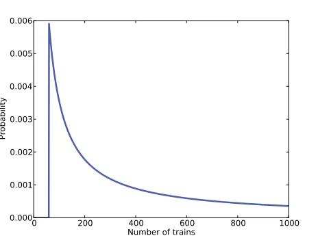
3.2 The locomotive problem
3.2. The locomotive problem 23
0 200 400 600 800 1000
Number of trains 0.000
0.001 0.002 0.003 0.004 0.005 0.006
Probability
Figure 3.1: Posterior distribution for the locomotive problem, based on a uniform prior.
A railroad numbers its locomotives in order 1..N. One day you see a locomotive with the number 60. Estimate how many locomotives the railroad has.
Based on this observation, we know the railroad has 60 or more locomotives. But how many more? To apply Bayesian reasoning, we can break this problem into two steps:
1. What did we know about N before we saw the data?
2. For any given value of N, what is the likelihood of seeing the data (a
locomotive with number 60)?
The answer to the rst question is the prior. The answer to the second is the likelihood.
We don't have much basis to choose a prior, but we can start with something
simple and then consider alternatives. Let's assume that N is equally likely
to be any value from 1 to 1000. hypos = xrange(1, 1001)
Now all we need is a likelihood function. In a hypothetical eet of N
loco-motives, what is the probability that we would see number 60? If we assume that there is only one train-operating company (or only one we care about) and that we are equally likely to see any of its locomotives, then the chance of seeing any particular locomotive is 1/N.
24 Chapter 3. Estimation
class Train(Suite):
def Likelihood(self, data, hypo): if hypo < data:
return 0 else:
return 1.0/hypo
This might look familiar; the likelihood functions for the locomotive problem and the dice problem are identical.
Here's the update:
suite = Train(hypos) suite.Update(60)
There are too many hypotheses to print, so I plotted the results in Figure 3.1. Not surprisingly, all values of N below 60 have been eliminated.
The most likely value, if you had to guess, is 60. That might not seem like a very good guess; after all, what are the chances that you just happened to see the train with the highest number? Nevertheless, if you want to maximize the chance of getting the answer exactly right, you should guess 60.
But maybe that's not the right goal. An alternative is to compute the mean of the posterior distribution:
def Mean(suite): total = 0
for hypo, prob in suite.Items(): total += hypo * prob
return total
print Mean(suite)
Or you could use the very similar method provided by Pmf: print suite.Mean()
The mean of the posterior is 333, so that might be a good guess if you wanted to minimize error. If you played this guessing game over and over, using the mean of the posterior as your estimate would minimize the mean squared error over the long run (see http://en.wikipedia.org/wiki/Minimum_mean_square_ error).
3.3. What about that prior? 25
3.3 What about that prior?
To make any progress on the locomotive problem we had to make assumptions, and some of them were pretty arbitrary. In particular, we chose a uniform prior from 1 to 1000, without much justication for choosing 1000, or for choosing a uniform distribution.
It is not crazy to believe that a railroad company might operate 1000 locomo-tives, but a reasonable person might guess more or fewer. So we might wonder whether the posterior distribution is sensitive to these assumptions. With so little dataonly one observationit probably is.
Recall that with a uniform prior from 1 to 1000, the mean of the posterior is 333. With an upper bound of 500, we get a posterior mean of 207, and with an upper bound of 2000, the posterior mean is 552.
So that's bad. There are two ways to proceed:
Get more data.
Get more background information.
With more data, posterior distributions based on dierent priors tend to con-verge. For example, suppose that in addition to train 60 we also see trains 30 and 90. We can update the distribution like this:
for data in [60, 30, 90]: suite.Update(data)
With these data, the means of the posteriors are Upper Posterior
Bound Mean
500 152
1000 164
2000 171
So the dierences are smaller.
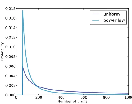
3.4 An alternative prior
26 Chapter 3. Estimation
0 200 400 600 800 1000
Number of trains 0.000
0.002 0.004 0.006 0.008 0.010 0.012 0.014 0.016 0.018
Probability
uniform power law
Figure 3.2: Posterior distribution based on a power law prior, compared to a uniform prior.
With some eort, we could probably nd a list of companies that operate locomotives in the area of observation. Or we could interview an expert in rail shipping to gather information about the typical size of companies.
But even without getting into the specics of railroad economics, we can make some educated guesses. In most elds, there are many small companies, fewer medium-sized companies, and only one or two very large companies. In fact, the distribution of company sizes tends to follow a power law, as Robert Axtell reports in Science (see http://www.sciencemag.org/content/293/ 5536/1818.full.pdf).
This law suggests that if there are 1000 companies with fewer than 10 locomo-tives, there might be 100 companies with 100 locomolocomo-tives, 10 companies with 1000, and possibly one company with 10,000 locomotives.
Mathematically, a power law means that the number of companies with a given size is inversely proportional to size, or
PMF(x)∝
1 x
α
wherePMF(x)is the probability mass function ofxandα is a parameter that
is often near 1.
3.5. Credible intervals 27
def __init__(self, hypos, alpha=1.0): Pmf.__init__(self)
for hypo in hypos:
self.Set(hypo, hypo**(-alpha)) self.Normalize()
And here's the code that constructs the prior: hypos = range(1, 1001)
suite = Train(hypos)
Again, the upper bound is arbitrary, but with a power law prior, the posterior is less sensitive to this choice.
Figure 3.2 shows the new posterior based on the power law, compared to the posterior based on the uniform prior. Using the background information represented in the power law prior, we can all but eliminate values ofN greater
than 700.
If we start with this prior and observe trains 30, 60, and 90, the means of the posteriors are
Upper Posterior Bound Mean
500 131
1000 133
2000 134
Now the dierences are much smaller. In fact, with an arbitrarily large upper bound, the mean converges on 134.
So the power law prior is more realistic, because it is based on general infor-mation about the size of companies, and it behaves better in practice.
You can download the examples in this section from http://thinkbayes. com/train3.py. For more information see Section 0.3.
3.5 Credible intervals
Once you have computed a posterior distribution, it is often useful to summa-rize the results with a single point estimate or an interval. For point estimates it is common to use the mean, median, or the value with maximum likelihood.
28 Chapter 3. Estimation
A simple way to compute a credible interval is to add up the probabilities in the posterior distribution and record the values that correspond to probabilities 5% and 95%. In other words, the 5th and 95th percentiles.
thinkbayes provides a function that computes percentiles: def Percentile(pmf, percentage):
p = percentage / 100.0 total = 0
for val, prob in pmf.Items(): total += prob
if total >= p: return val And here's the code that uses it:
interval = Percentile(suite, 5), Percentile(suite, 95) print interval
For the previous examplethe locomotive problem with a power law prior
and three trainsthe 90% credible interval is (91,243). The width of this
range suggests, correctly, that we are still quite uncertain about how many locomotives there are.
3.6 Cumulative distribution functions
In the previous section we computed percentiles by iterating through the values and probabilities in a Pmf. If we need to compute more than a few percentiles, it is more ecient to use a cumulative distribution function, or Cdf.
Cdfs and Pmfs are equivalent in the sense that they contain the same informa-tion about the distribuinforma-tion, and you can always convert from one to the other. The advantage of the Cdf is that you can compute percentiles more eciently. thinkbayes provides a Cdf class that represents a cumulative distribution function. Pmf provides a method that makes the corresponding Cdf:
cdf = suite.MakeCdf()
And Cdf provides a function named Percentile
interval = cdf.Percentile(5), cdf.Percentile(95)
3.7. The German tank problem 29
up a value to get the corresponding probability is also logarithmic, so Cdfs are ecient for many calculations.
The examples in this section are in http://thinkbayes.com/train3.py. For more information see Section 0.3.
3.7 The German tank problem
During World War II, the Economic Warfare Division of the American Em-bassy in London used statistical analysis to estimate German production of tanks and other equipment.1
The Western Allies had captured log books, inventories, and repair records that included chassis and engine serial numbers for individual tanks.
Analysis of these records indicated that serial numbers were allocated by man-ufacturer and tank type in blocks of 100 numbers, that numbers in each block were used sequentially, and that not all numbers in each block were used. So the problem of estimating German tank production could be reduced, within each block of 100 numbers, to a form of the locomotive problem.
Based on this insight, American and British analysts produced estimates sub-stantially lower than estimates from other forms of intelligence. And after the war, records indicated that they were substantially more accurate.
They performed similar analyses for tires, trucks, rockets, and other equip-ment, yielding accurate and actionable economic intelligence.
The German tank problem is historically interesting; it is also a nice example of real-world application of statistical estimation. So far many of the examples in this book have been toy problems, but it will not be long before we start solving real problems. I think it is an advantage of Bayesian analysis, especially with the computational approach we are taking, that it provides such a short path from a basic introduction to the research frontier.
3.8 Discussion
Among Bayesians, there are two approaches to choosing prior distributions. Some recommend choosing the prior that best represents background infor-mation about the problem; in that case the prior is said to be informative.
1Ruggles and Brodie, An Empirical Approach to Economic Intelligence in World War
30 Chapter 3. Estimation
The problem with using an informative prior is that people might use dier-ent background information (or interpret it dierdier-ently). So informative priors often seem subjective.
The alternative is a so-called uninformative prior, which is intended to be as unrestricted as possible, in order to let the data speak for themselves. In some cases you can identify a unique prior that has some desirable property, like representing minimal prior information about the estimated quantity. Uninformative priors are appealing because they seem more objective. But I am generally in favor of using informative priors. Why? First, Bayesian analysis is always based on modeling decisions. Choosing the prior is one of those decisions, but it is not the only one, and it might not even be the most subjective. So even if an uninformative prior is more objective, the entire analysis is still subjective.
Also, for most practical problems, you are likely to be in one of two regimes: either you have a lot of data or not very much. If you have a lot of data, the choice of the prior doesn't matter very much; informative and uninformative priors yield almost the same results. We'll see an example like this in the next chapter.
But if, as in the locomotive problem, you don't have much data, using rel-evant background information (like the power law distribution) makes a big dierence.
And if, as in the German tank problem, you have to make life-and-death deci-sions based on your results, you should probably use all of the information at your disposal, rather than maintaining the illusion of objectivity by pretending to know less than you do.
3.9 Exercises
Exercise 3.1 To write a likelihood function for the locomotive problem, we
had to answer this question: If the railroad has N locomotives, what is the
probability that we see number 60?
The answer depends on what sampling process we use when we observe the locomotive. In this chapter, I resolved the ambiguity by specifying that there is only one train-operating company (or only one that we care about).
3.9. Exercises 31
any company. In that case, the likelihood function is dierent because you are more likely to see a train operated by a large company.
Chapter 4
More Estimation
4.1 The Euro problem
In Information Theory, Inference, and Learning Algorithms, David MacKay poses this problem:
A statistical statement appeared in The Guardian" on Friday Jan-uary 4, 2002:
When spun on edge 250 times, a Belgian one-euro coin came up heads 140 times and tails 110. `It looks very suspicious to me,' said Barry Blight, a statistics lecturer at the London School of Economics. `If the coin were unbiased, the chance of getting a result as extreme as that would be less than 7%.'
But do these data give evidence that the coin is biased rather than fair?
To answer that question, we'll proceed in two steps. The rst is to estimate the probability that the coin lands face up. The second is to evaluate whether the data support the hypothesis that the coin is biased.
You can download the code in this section from http://thinkbayes.com/ euro.py. For more information see Section 0.3.
Any given coin has some probability, x, of landing heads up when spun on
edge. It seems reasonable to believe that the value of x depends on some
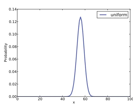
34 Chapter 4. More Estimation
0 20 40 x 60 80 100
0.00 0.02 0.04 0.06 0.08 0.10 0.12 0.14
Probability
uniform
Figure 4.1: Posterior distribution for the Euro problem on a uniform prior.
If a coin is perfectly balanced, we expect x to be close to 50%, but for a
lopsided coin,x might be substantially dierent. We can use Bayes's theorem
and the observed data to estimatex.
Let's dene 101 hypotheses, where Hx is the hypothesis that the probability
of heads isx%, for values from 0 to 100. I'll start with a uniform prior where
the probability ofHx is the same for all x. We'll come back later to consider
other priors.
The likelihood function is relatively easy: If Hx is true, the probability of
heads isx/100 and the probability of tails is 1−x/100.
class Euro(Suite):
def Likelihood(self, data, hypo): x = hypo
if data == 'H': return x/100.0 else:
return 1 - x/100.0
Here's the code that makes the suite and updates it: suite = Euro(xrange(0, 101))
dataset = 'H' * 140 + 'T' * 110
4.2. Summarizing the posterior 35
4.2 Summarizing the posterior
Again, there are several ways to summarize the posterior distribution. One option is to nd the most likely value in the posterior distribution. thinkbayes provides a function that does that:
def MaximumLikelihood(pmf):
"""Returns the value with the highest probability.""" prob, val = max((prob, val) for val, prob in pmf.Items()) return val
In this case the result is 56, which is also the observed percentage of heads,
140/250 = 56%. So that suggests (correctly) that the observed percentage is
the maximum likelihood estimator for the population.
We might also summarize the posterior by computing the mean and median: print 'Mean', suite.Mean()
print 'Median', thinkbayes.Percentile(suite, 50)
The mean is 55.95; the median is 56. Finally, we can compute a credible interval:
print 'CI', thinkbayes.CredibleInterval(suite, 90) The result is (51,61).
Now, getting back to the original question, we would like to know whether the coin is fair. We observe that the posterior credible interval does not include 50%, which suggests that the coin is not fair.
But that is not exactly the question we started with. MacKay asked, Do these data give evidence that the coin is biased rather than fair? To answer that question, we will have to be more precise about what it means to say that data constitute evidence for a hypothesis. And that is the subject of the next chapter.
But before we go on, I want to address one possible source of confusion. Since we want to know whether the coin is fair, it might be tempting to ask for the probability that x is 50%:
print suite.Prob(50)
36 Chapter 4. More Estimation
0 20 40 x 60 80 100
0.000 0.005 0.010 0.015 0.020 0.025
Probability
uniform triangle
Figure 4.2: Uniform and triangular priors for the Euro problem.
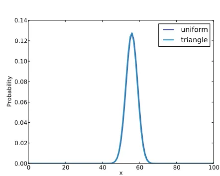
0 20 40 x 60 80 100
0.00 0.02 0.04 0.06 0.08 0.10 0.12 0.14
Probability
uniform triangle
4.3. Swamping the priors 37
4.3 Swamping the priors
We started with a uniform prior, but that might not be a good choice. I can believe that if a coin is lopsided, x might deviate substantially from 50%, but
it seems unlikely that the Belgian Euro coin is so imbalanced that xis 10% or
90%.
It might be more reasonable to choose a prior that gives higher probability to values of xnear 50% and lower probability to extreme values.
As an example, I constructed a triangular prior, shown in Figure 4.2. Here's the code that constructs the prior:
def TrianglePrior(): suite = Euro()
for x in range(0, 51): suite.Set(x, x) for x in range(51, 101):
suite.Set(x, 100-x) suite.Normalize()
Figure 4.2 shows the result (and the uniform prior for comparison). Updating this prior with the same dataset yields the posterior distribution shown in Figure 4.3. Even with substantially dierent priors, the posterior distributions are very similar. The medians and the credible intervals are identical; the means dier by less than 0.5%.
This is an example of swamping the priors: with enough data, people who start with dierent priors will tend to converge on the same posterior.
4.4 Optimization
The code I have shown so far is meant to be easy to read, but it is not very ecient. In general, I like to develop code that is demonstrably correct, then check whether it is fast enough for my purposes. If so, there is no need to optimize. For this example, if we care about run time, there are several ways we can speed it up.
The rst opportunity is to reduce the number of times we normalize the suite. In the original code, we call Update once for each spin.
dataset = 'H' * heads + 'T' * tails
38 Chapter 4. More Estimation
And here's what Update looks like: def Update(self, data):
for hypo in self.Values():
like = self.Likelihood(data, hypo) self.Mult(hypo, like)
return self.Normalize()
Each update iterates through the hypotheses, then calls Normalize, which iterates through the hypotheses again. We can save some time by doing all of the updates before normalizing.
Suite provides a method called UpdateSet that does exactly that. Here it is: def UpdateSet(self, dataset):
for data in dataset:
for hypo in self.Values():
like = self.Likelihood(data, hypo) self.Mult(hypo, like)
return self.Normalize() And here's how we can invoke it:
dataset = 'H' * heads + 'T' * tails suite.UpdateSet(dataset)
This optimization speeds things up, but the run time is still proportional to the amount of data. We can speed things up even more by rewriting Likelihood to process the entire dataset, rather than one spin at a time.
In the original version, data is a string that encodes either heads or tails: def Likelihood(self, data, hypo):
x = hypo / 100.0 if data == 'H':
return x else:
return 1-x
As an alternative, we could encode the dataset as a tuple of two integers: the number of heads and tails. In that case Likelihood looks like this:
def Likelihood(self, data, hypo): x = hypo / 100.0
heads, tails = data
like = x**heads * (1-x)**tails return like
4.5. The beta distribution 39
heads, tails = 140, 110 suite.Update((heads, tails))
Since we have replaced repeated multiplication with exponentiation, this ver-sion takes the same time for any number of spins.
4.5 The beta distribution
There is one more optimization that solves this problem even faster.
So far we have used a Pmf object to represent a discrete set of values for x. Now we will use a continuous distribution, specically the beta distribution (see http://en.wikipedia.org/wiki/Beta_distribution).
The beta distribution is dened on the interval from 0 to 1 (including both), so it is a natural choice for describing proportions and probabilities. But wait, it gets better.
It turns out that if you do a Bayesian update with a binomial likelihood function, which is what we did in the previous section, the beta distribution is a conjugate prior. That means that if the prior distribution for x is a beta distribution, the posterior is also a beta distribution. But wait, it gets even better.
The shape of the beta distribution depends on two parameters, writtenα and
β, or alpha and beta. If the prior is a beta distribution with parameters
alpha and beta, and we see data with h heads and t tails, the posterior is a beta distribution with parameters alpha+h and beta+t. In other words, we can do an update with two additions.
So that's great, but it only works if we can nd a beta distribution that is a good choice for a prior. Fortunately, for many realistic priors there is a beta distribution that is at least a good approximation, and for a uniform prior there is a perfect match. The beta distribution with alpha=1 and beta=1 is uniform from 0 to 1.
Let's see how we can take advantage of all this. thinkbayes.py provides a class that represents a beta distribution:
class Beta(object):
def __init__(self, alpha=1, beta=1): self.alpha = alpha
40 Chapter 4. More Estimation
By default __init__ makes a uniform distribution. Update performs a Bayesian update:
def Update(self, data): heads, tails = data self.alpha += heads self.beta += tails
data is a pair of integers representing the number of heads and tails. So we have yet another way to solve the Euro problem:
beta = thinkbayes.Beta() beta.Update((140, 110)) print beta.Mean()
Beta provides Mean, which computes a simple function of alpha and beta: def Mean(self):
return float(self.alpha) / (self.alpha + self.beta) For the Euro problem the posterior mean is 56%, which is the same result we got using Pmfs.
Beta also provides EvalPdf, which evaluates the probability density function (PDF) of the beta distribution:
def EvalPdf(self, x):
return x**(self.alpha-1) * (1-x)**(self.beta-1)
Finally, Beta provides MakePmf, which uses EvalPdf to generate a discrete approximation of the beta distribution.
4.6 Discussion
In this chapter we solved the same problem with two dierent priors and found that with a large dataset, the priors get swamped. If two people start with dierent prior beliefs, they generally nd, as they see more data, that their posterior distributions converge. At some point the dierence between their distributions is small enough that it has no practical eect.
When this happens, it relieves some of the worry about objectivity that I discussed in the previous chapter. And for many real-world problems even stark prior beliefs can eventually be reconciled by data.