Quantum effects in warp drives
Stefano Finazzi1,a
1INO-CNR BEC Center and Dipartimento di Fisica, Universita di Trento, via Sommarive 14, 38123
Povo-Trento, Italy
Abstract.Warp drives are interesting configurations that, at least theoretically, provide a way to travel at superluminal speed. Unfortunately, several issues seem to forbid their realization. First, a huge amount of exotic matter is required to build them. Second, the presence of quantum fields propagating in superluminal warp-drive geometries makes them semiclassically unstable. Indeed, a Hawking-like high-temperature flux of parti-cles is generated inside the warp-drive bubble, which causes an exponential growth of the energy density measured at the front wall of the bubble by freely falling observers. More-over, superluminal warp drives remain unstable even if the Lorentz symmetry is broken by the introduction of regulating higher order terms in the Lagrangian of the quantum field. If the dispersion relation of the quantum field is subluminal, a black-hole laser phe-nomenon yields an exponential amplification of the emitted flux. If it is superluminal, infrared effects cause a linear growth of this flux.
1 Introduction
A warp drive [1] can be defined as a bubble of spacetime moving in an asymptotically flat spacetime at an arbitrary speed. This configuration provides both a way to travel at superluminal speeds and an exciting ground to test our comprehension of general relativity (GR) and quantum field theory in curved spacetimes (for instance when investigating warp-drive implications for causality [2]). Their geometry is defined by the line element
ds2=−c2dt2+[dx−v(r)dt]2+dy2+dz2, (1)
wherer≡ p(x−v0t)2+y2+z2parametrizes the distance from the center of the bubble andv0is the
warp-drive velocity. The functionvsatisfiesv(0)=v0andv(r)→0 forr→ ∞.
When this metric is put into Einstein’s equations, it is apparent that a large amount of exotic matter (i.e., matter that violates energy conditions, see Ref. [3] for a complete review about “exotic spacetimes”) is required to stretch the spacetime around the warp-drive bubble. Surprisingly, exotic matter is needed to sustain warp drives moving not only with superluminal speeds, but also with subluminal ones [4, 5]. Furthermore, the amount of exotic matter is related to both the size of the warp-drive bubble and the thickness of the bubble walls [6]. If the exoticity is provided by quantum fields, satisfying therefore the so-called quantum inequalities (QI—see [7] for a review about QI applied to exotic spacetimes), then the violations of the energy conditions must be confined to Planck-size
ae-mail: [email protected]
/
C
regions. Accordingly, the thickness∆of the wall of the bubble is of Planck size [∆≤102(v 0/c)LP,
whereLP is the Planck length]. Unfortunately, to support a warp-drive bubble with such thin walls,
a size of about 100 m, and propagating atv0 ≈c, a huge amount of exotic matter is required,|E−|
1011M. Modified configurations with a reduced surface area but the same bubble volume [8] can reduce the amount of negative energy (|E−| ≈ 0.3M for a 100 m-radius bubble), although some positive energy must be added outside the bubble (E+≈2.5M).
Regarding the feasibility of warp-drive configurations, a parallel line of research has focused on the study of their semiclassical stability against the introduction of quantum fields propagating on these geometries. In Ref. [9] this issue was studied in the case of an eternal superluminal warp drive. It was noticed that, for an observer within the warp-drive bubble, the backward and forward walls (along the direction of motion) look like the horizon of a black hole and of a white hole, respectively. By imposing a quantum state which is vacuum at the null infinities (that is, the analog of the Boulware state for an eternal black hole) it was found that the renormalized stress-energy tensor (RSET) diverges at the horizons (see Ref. [10] for a different point of view). Thus, the divergence of the RSET at the horizons makes superluminal warp drives unstable within the context of semiclassical GR.
In a more realistic situation, a warp drive is dynamically created at a finite timetHwith a very low
velocity and then accelerated to superluminal speeds. In this case the quantum state is globally fixed by suitable boundary conditions at early times, before the formation of the warp-drive bubble. This situation is similar to the formation of a black hole through a gravitational collapse. In the black hole case, the globally defined quantum state that is vacuum onI−is regular on the horizon and thermal onI+. In other words, the dynamics of a collapse end up selecting a quantum state that at late times resembles the Unruh state defined on eternal black holes, rather than a Boulware-like state.
In this contribution we summarize the results of three works [11–13] investigating the semiclas-sical stability properties of warp drives. In Sec. 2 we analyze the causal structure on an eternal warp drive and of a warp drive which is dynamically created with zero velocity and then accelerated up to superluminal speed in a finite amount of time. In this latter configuration, where a proper quantum state can be unambiguously defined, we investigate the properties of spontaneous quantum vacuum emission by calculating the RSET inside the warp-drive bubble (Sec. 3). In the center of the bubble we find a thermal flux at the Hawking temperature corresponding to the surface gravity of the black horizon. Furthermore, the RSET grows exponentially with time on the white horizon. This makes warp drives unstable once superluminal speeds are reached.
However, this analysis rests on relativistic quantum field theory. Thus, one may wonder whether this instability is peculiar to the assumed local Lorentz symmetry. For instance, it is known that non-linear dispersion relations remove Cauchy horizons and regulate the fluxes emitted by white holes [14]. To clarify this issue, in Sec. 4, this stability analysis is extended to a quantum field theory where Lorentz invariance is broken at ultra-high energy [13]. Even if the exponential growth of the RSET on the white hole is in fact removed, new types of instability appear, whose properties depend on the form of the dispersion relation of the quantum field.
2 The warp-drive geometry
2.1 Causal structure
The geometrical and causal properties of warp-drive spacetimes are more conveniently investigated by restricting to the 1+1 dimensional case using a new spatial coordinater≡x−v0tin the metric of
Eq. (1),
where ¯v =v−v0. We putv=v0f(r), where f(r) is a smooth function with maximum f(0) =1 and
f(r) → 0 forr → ±∞. Therefore, ¯vhas a maximum inr = 0, where it vanishes, and goes to the constant value−v0<−cforr→ ±∞. Consequently there are two positionsrBandrWwhere|v¯|=c.
A possible choice of ¯vsatisfying these conditions is plotted in Fig. 1. As seen from an observer inside the bubble,rB andrW correspond to a black and a white hole horizons,HB andHW, respectively,
separating the spacetime in three regions: L, appearing as the interior of the black hole, C, appearing as the exterior of both the black and the white hole, and R, appearing as the interior of the white hole (see Fig. 1).
-1 0
rW
rB
r
L C R
¯
v
Figure 1. Velocity profile for a rightgoing warp drive [see Eq.(2)]. Twosuperluminalasymptotic regions L and R are separated by a black and a white horizon from a compact internalsubluminal region C. The Killing field∂tis space-like in L and
R, light-like on both horizons, and time-like in C.
i+ i− i0 L i0 R I+L
(t= + ∞,r=
−∞) IL+(t = +∞
,r=
−∞)
H+ C(t
= +∞ ,r=
rW)
H+ R(t
= +∞ ,r=
r W) H − L(t = −∞, r= rB)
H− C(t =
−∞,
r= rB)
I−R
(t= −∞,
r= + ∞) IR−(t
= −∞, r = +∞ ) HB HW (r= rB)
(r= rW) t=
const r=con
st
r=con st r = con st H+ z }| { | {z } H−
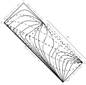
Figure 2. Penrose diagram of an eternal warp drive. Lines of constantr(solid lines) and of con-stantt(dashed lines). Future and past horizons at r =rB,W (heavy dashed lines). The geometry can
be extended to the future ofH+(formed byHC+ andHR+) and to the past ofH−(formed byHC− andHL−).
The Penrose diagram of a warp drive is therefore obtained by pasting together the diagrams of a black hole, on the left, and of a white hole, on the right. Note that this diagram does not represent the maximal analytical extension of this spacetime: The dashed linesH−(formed byHC−andHL−) andH+(formed byHC+andHR+) signal the locations at which the geometry can be extended.HC− andHC+correspond to the past and future horizons in the Penrose diagrams of an eternal black and white hole, respectively. While in the black hole case a maximal extension is well known for vac-uum solutions such as the Schwarzschild or Kerr spacetimes, for a warp-drive geometry the maximal extension cannot be uniquely determined because the distribution of matter is unknown beyondH±, which behave like Cauchy horizons.
Hence, because of the presence of the past Cauchy horizonH−, a quantum state with appropriate initial conditions cannot be imposed at t → −∞. However, in a realistic situation, a warp-drive geometry is not eternal but it is dynamically formed at some finite timetH. Before tH the causal
structure of the spacetime is Minkowskian and proper boundary conditions can be chosen.
This dynamical warp-drive geometry is described by a metric of the form of Eq. (2), by replacing the constant velocity ¯vwith a time dependent velocity ˆv(t,r), satisfying ˆv(t,r) →0, fort → −∞and ˆ
it progressively changes tillt=tH, when the horizon forms. AftertH, the Penrose diagram coincides
with that of a stationary warp drive (Fig. 2). With respect to the eternal case, the past Cauchy horizon
H−has disappeared but the geometry can still be extended in the future, beyond the Cauchy horizons
H+
C andHR+. There exist indeed observers moving on time-like lines that reachHC+andHR+in a
finite proper time.
i+
i− i0L
i0 R I+L(t
=+∞ ,r=
−∞)
IL+(t
=+
∞ ,r=
−∞)
H+
C(t
=+
∞ ,r=
rW)
H+
R( t=
+∞ ,r=
rW)
I−R(t =−∞
,r= +∞)
IL−(t= −∞,r
=
−∞) H+B
H−W r= rB r= r W t= const
r=con
st r= cons t r =co nst H+ z }| {
Figure 3. Penrose diagram of a dynamic warp drive. Lines of constantr(solid lines) and of con-stantt(dashed lines). The lines of constantr be-come null at the apparent horizons (heavy dashed lines).
r
t
Figure 4.Light rays propagating rightward (solid lines) and leftward (dashed lines) in the plane (t,r) in a warp-drive spacetime defined by the velocity profile of Eq. (3). Heavy solid lines represent the functionsr(t)=±ξ(t)=±arccosh(t+1) used to im-plement the dynamical formation of the warp drive. Att<0 the metric is Minkowskian. The horizons atrBandrW(heavy dashed lines) appear attH=1.
2.2 Light-ray propagation
The presence of a black hole horizon in a superluminal warp-drive geometry suggests the possibility that Hawking-like radiation is produced. To investigate this phenomenon, we first study how light rays are bended by the warp-drive geometry, in particular we determine the relationU=p(u) between pastUand futureunull affine coordinates [15]. This information is indeed sufficient to investigate the properties of particle creation [16]. For illustrative purposes, in Fig. 4 we plot the rightgoing (solid line) and leftgoing (dashed lines) null geodesics propagating in a warp-drive geometry, defined by the following velocity profile (c=1),
ˆ
v(r,t)=
0 if t≤0, ¯
v[ξ(t)] if t>0 and|r| ≥ξ(t), ¯
v(r) if t>0 and|r|< ξ(t),
(3)
with
ξ(t)=arccosh(t+1) (4)
and
¯ v(r)=2
"
1 cosh(r)−1
#
. (5)
To determine the general relationU= p(u), we start from the differential equation for the propa-gation of rightgoing light rays
dr
dt =c+ˆv(r,t). (6)
Since forttHthe velocity profile ˆv=¯vdepends only onr, the late-time null coordinateuis defined
by
du=dt− dr
c+v¯(r). (7)
We now restrict to the central region C. Here the asymptotic form is found by integrating the above equation in the limitr→rB,W, where the velocity ¯vis
¯
v=−c±κB,W r−rB,W
+O
r−rB,W
2
(8)
and
κB,W≡
d¯v dr r=r
B,W
(9)
are the surface gravities of the black horizon and of the white horizon, respectively. For the sake of simplicity, from now on we assume that they have the same valueκB,W=κ, without loss of generality.
We obtain
u't∓1
κ lnr−rB,W. (10)
The early-time null coordinateU, obtained by integrating Eq. (6) when ˆv=0, reduces to
U(t→ −∞)=t−r
c, (11)
in the limitt→ ∞. This coordinate is regular everywhere, in particular on the horizons. Consequently, on atslice in the late-time stationary region,Ucan be written as
UB,W=UB,W r−rB,W
,
(12)
whereUB,W denotes the specific form ofU close to the black and white horizon, respectively, and
UB,Ware analytic functions. Putting Eq. (10) into the above expression,
UB,W =p(u→ ±∞)=PB,W(e∓κu), (13)
wherePB,W are analytic functions. Close to the horizonsu → ±∞, thus e∓κu → 0 and p can be
expanded as
U=p(u→ ±∞)=UB,W∓AB,We∓κu+O
e∓2κu , (14)
whereAB,W are positive constants. This asymptotic behavior of rightgoing rays is apparent from
Fig. 4 (solid lines). It yields exponential separation of null geodesic close to the black horizon and exponential accumulation close to the white horizon.
It is worth stressing that this result is completely general. The asymptotic form ofU = p(u) does not depend on the details of ˆv, but only on its early- and late-time behaviors, corresponding to a Minkowskian spacetime at and to a stationary warp-drive spacetime, respectively.
Analogously, one can find the relation between the early- and late-times null coordinatesW and w, associated with leftgoing light rays, which are solutions of
dr
In this case, leftgoing rays can cross the horizons, propagating fromIR−toIL+(see Figs. 3 and 4). As a consequence, bothW andware defined in the asymptotic regions L and R outside the bubble. For instance,
W(t→ −∞)=t+r
c. (16)
However, in place ofw, it is more convenient to use a different coordinate ˜w, defined inside the bubble in analogy with Eq. (7),
d ˜w=dt+ dr
c−v¯(r). (17)
It is easy to show [11] that the relationW = q( ˜w) is always regular, as illustrated in Fig. 4 by the non-singular behavior of leftgoing null geodesics (dashed lines).
3 Particle production and renormalized stress-energy tensor
In a black hole geometry an exponential relationp(U) betweenuandU, as in Eq. (14), allows to conclude that Hawking radiation is emitted with temperatureκ/2π. However, in the case of warp drives, its implications for particle production are not straightforward because late-time modes labeled byuare not standard plane waves [see Eq. (10)]. Only ifκis large enough that the typical wavelength of the emitted radiation is much smaller than the bubble size, then a plane-wave approximation is allowed in the center of the bubble. In this case, it is possible to conclude that standard Hawking radiation at temperatureT is emitted at late times. To obtain more significant information, also close to the horizons, we therefore consider the behavior of the RSET.
To calculate the RSET inside the warp-drive bubble we follow the method proposed in [17]. The metric can be written as
ds2=−C(U,W)dUdW. (18)
or, using the null coordinatesuand ˜w, as
ds2=−C¯(u,w˜)dud ˜w , C(U,W)= C¯(u,w˜) ˙
p(u) ˙q( ˜w), (19)
whereU = p(u) andW =q( ˜w). Following Ref. [11], we refer to the RSET associated with a single quantum massless scalar field. Its components are [16]:
TUU =−
1
12πC1/2∂2UC−
1/2, (20)
TWW =−
1 12πC
1/2∂2
WC−
1/2, (21)
TUW =TWU =
1
96πC R. (22)
In the presence of other fields, the previous expressions have to be corrected only by a multiplica-tive numerical factor. The RSET components in the stationary region inside the bubble are directly computed by using the relationshipsU=p(u) andW=q( ˜w), introduced in Sec. 2.2.
Significant physical information is extracted from the RSET by studying, for instance, the en-ergy densityρmeasured by a set of freely falling observers, with four velocityuµ = (1,v¯) in (t,r) coordinates,
which is conveniently expressed as the sum of three terms,
ρ=ρst+ρdyn−u+ρdyn−w.˜ (24)
The first static term
ρst≡ −
1 24π
¯
v4−¯v2+2
1−v¯22 v¯
02+ 2¯v
1−v¯2v¯
00
(25)
depends only on thercoordinate through ¯v(r) and represent vacuum polarization. The two dynamical terms
ρdyn−u≡
1 48π
f(u)
(1+v¯)2, (26)
ρdyn−w˜ ≡
1 48π
g(w)
(1−v¯)2 (27)
depend also onu ( ˜w) and correspond to the energy carried by rightgoing (leftgoing) rays, which is red/blue-shifted by a term depending onr. To keep the notation compact we have putc=1 and we have defined
f(u)≡3 ¨p
2(u)−2 ˙p(u)...p(u)
˙
p2(u) , (28)
g( ˜w)≡3 ¨q2( ˜w)−2 ˙q( ˜w)
...
q( ˜w)
˙
q2( ˜w) . (29)
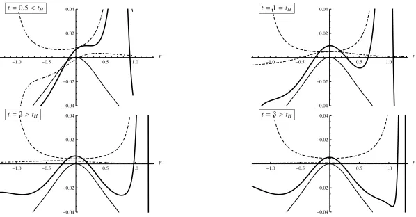
In Fig. 5, we present the result of the calculation ofρinside the bubble [12], for a warp-drive geometry defined by the velocity profile introduced in Eq. (3). With this choice, the surface gravity isκ = √3/2 and the horizons appear attH =1. The energy densityρ(thick solid line) of Eq. (23)
is plotted as a function ofrat different times (t = 0.5,1,2,3) andrvaries betweenrB andrW, the
locations ofHWandHB. The three termsρst,ρdyn−u, andρdyn−w, defined in Eqs. (25), (26), and (27),
are plotted with thin-solid, dashed, and dot-dashed lines, respectively.
-1.0 -0.5 0.5 1.0
-0.04 -0.02 0.02 0.04
r t=0.5<tH
-1.0 -0.5 0.5 1.0
-0.04 -0.02 0.02 0.04
r t=1=tH
-1.0 -0.5 0.5 1.0
-0.04 -0.02 0.02 0.04
r t=2>tH
-1.0 -0.5 0.5 1.0
-0.04 -0.02 0.02 0.04
r t=3>tH
Figure 5.Energy densityρ(thick solid line),ρst(solid line),ρdyn−u(dashed line) andρdyn−w(dot-dashed line) as
This figure shows that the dynamic termρdyn−w(dot-dashed line) is transient and gives an
impor-tant contribution only during the process of formation of the warp-drive bubble. In fact,g( ˜w) differs from 0 only for values of ˜wcorresponding to light rays crossing the bubble att ∼ tH. At late time
instead ˙q( ˜w) goes to a constant andg( ˜w)→0. Thus,ρdyn−wcan be safely neglected at late times.
RSET in the center of the bubble.
In the center of the bubble (r = 0)ρst =0, because ¯v(r = 0) = ¯v0(r =0) =0. At late times when
ρdyn−w is negligible, the only contribution to the energy density is given here byρdyn−u. Moreover,
sinceu(t,0) →+∞,ρdyn−ucan be evaluated by expanding f(u) at large values ofu, f(u→ ∞)=κ2.
Finallyρ(r=0)≈κ2/(48π). This is the energy densityπT2
H/12 of a scalar field in 1+1 dimensions
at the Hawking temperatureTH=κ/2π. Usingκ=
√
3/2, the energy density isρ≈κ2/48π≈0.005,
which coincides with the numerical results at late times (t=3), shown in the bottom panel of Fig. 5. Note that the Hawking temperature of this radiation is huge,TH∼κ &10−2TP, whereTPis the
Planck temperature, about 1032K, when QI are assumed [6, 8]. Indeed, the wall thickness for a warp drive withv0 ≈cwould be∆.102LP, and its surface gravityκ &10−2t−P1, wheretPis the Planck
time. If instead the warp drive is supported by matter violating QI, such a high temperature can be avoided. For instance, with∆∼1 m, the temperature is about 0.003 K (corresponding to a wavelength of 1 m).
RSET on the black, white, and Cauchy horizons.
On the horizonsr=rB,W, bothρstandρdyn−udiverge. Indeed the term (1+¯v) in the denominators of
Eqs. (25) and (26) vanishes atr=rB,W. By expanding f(u) foru→ ±∞inρstandρdyn−u, one finds
that the diverging terms exactly cancel each other [11] and the totalρdoes not diverge, in agreement with the Fulling-Sweeny-Wald theorem [18]. Furthermore, the subleading terms yield
ρ r'rB,W=CB,W+BB,We∓2κt+O r−rB,W. (30)
This contribution is exponentially damped on the black horizon, on a time scale∼1/κ, as shown in Fig. 5. The same behavior characterizes the RSET on the horizon of a black hole formed through the gravitational collapse of a star [17]. Conversely, on the white horizon the subleading term exponen-tially grows with time. That is, moving alongHW,ρgrows exponentially and diverges at the crossing
point betweenHWandHC+, as shown in Fig. 5, where the value ofρ(thick solid line) atr=rWgoes
towards−∞ast→+∞.
Finally, a positive energy pulse, whose value at the peak diverges with time to+∞, approaches
rW asr−rW ∝e−κt. Thus,ρdiverges in two different ways forr → rW andt → ∞, depending on
the order in which the two limits are taken. To understand the physical meaning of these divergences it is convenient to consider the Penrose diagram of Fig. 3, where the location (r = rW,t = +∞)
is represented by a whole line (HC+andHR+) rather than by a single point. The former negative divergence appears by first taking the limitr → rW and afterwards moving on the white horizon
HWtoward the crossing point betweenHWandHC+(late-time limit). The latter positive divergence
appears instead by fixing a value ofuand moving on the corresponding geodesic, which is parallel toHB andHW in the Penrose diagram, until the Cauchy horizonHC+ is reached. Note that these
results do not contradict the Fulling-Sweeny-Wald theorem [18], since both divergences take place on a Cauchy horizon.
Furthermore, the natures of these two divergences are quite different. The divergence at the cross-ing point betweenHW andHC+is intrinsically due to the inevitable transient disturbances produced
blue-shift suffered by light rays as they approach the Cauchy horizon and it is similar to the often claimed instability of inner horizons in Kerr-Newman black holes [19–21].
However, in both cases these effects produce an exponential growth of the RSET, whose backre-action dooms the warp drive to be semiclassically unstable on a time scale of the order of 1/κ, the inverse of the surface gravity of the white horizon. By QI inequalities, this timescale would be of the order of 102Planck times, about 10−42 s. Even violating the QI, to get a time scale of 1 s, a wall as large as 3×10⁸m is needed. Thus, most probably, one would be able to maintain a warp drive with superluminal speed for a very short interval of time.
4 Warp drives in Lorentz violating theories
In the previous section we showed that superluminal warp-drive geometries are quantum mechani-cally unstable. However, that analysis rested on relativistic quantum field theory. Thus, one should examine whether the warp-drive instability is peculiar to the assumed local Lorentz symmetry. In-deed, it is known that non-linear dispersion relations remove Cauchy horizons and regulate the fluxes emitted by white holes [14]. Moreover, although observations constrain to ultra high energy a pos-sible breaking of that symmetry [22], one cannot definitely exclude ultraviolet violations of the local Lorentz symmetry, which have been suggested by several investigations [23–25].
A stability analysis of warp-drive configurations with Lorentz violation was performed in [13] in a 1+1 dimensional stationary system, by considering a massless scalar field with quartic dispersion relation propagating on a geometry defined by the line element of Eq. (2). If the Lorentz symmetry is violated, it is sufficient to consider stationary warp drives, because in this case the Cauchy horizons are not present and the initial quantum state can be properly defined without ambiguities. In this spacetime∂tis therefore a globally defined Killing vector field, which is time-like within the bubble
(region C) and space-like outside (regions L and R, see Fig. 1). The action of this scalar fields is
S±=1
2
Z
d2x√−g
"
gµν∂ µφ∂νφ±
(hµν∂µ∂νφ)2
Λ2
#
, (31)
wherehµν=gµν+uµuνis the spatial metric on a section orthogonal to some unit time-like vector field
uµ, which specifies the preferred frame used to implement the dispersion relation [26]. In the present settingsuµshould be given from the outset, while in condensed matter the preferred frame is fixed by the fluid flow [27]. Inspired by this analogy, we chooseuµto be (1,v¯) in the (t,r) frame. Thisuµflow is geodesic and asymptotically at rest in the (t,x) frame of Eq. (1), so that stationarity is preserved. The sign±in Eq. (31) holds for superluminal dispersion (velocity of high momentum photons larger than velocitycof low momentum photons) and subluminal dispersion (velocity of high momentum photons smaller thanc), respectively. With the metric of Eq. (2), the wave equation generated by the above action is "
(∂t+∂r¯v) (∂t+v∂¯ r)−∂2r±
1 Λ2∂
4
r
#
φ=0. (32)
Because of stationarity, the field can be decomposed in eigenfrequency modes φ = R dωe−iωtφω, whereωis the conserved frequency (with respect to the Killing time). Correspondingly, at fixedωthe dispersion relation reads
(ω−v¯kω)2 =k2ω± k
4
ω Λ2 ≡Ω
2
±, (33)
kΩu kΩw
k- ΩH2L k- ΩH1L
k W
k W
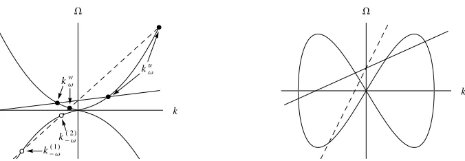
Figure 6.Graphical solution of Eq. (33) for super (top panel), and subluminal dispersion (bottom panel). In both panels, the straight lines representω−¯vkfor|v¯|<1 (solid) and|v¯| >1 (dashed). The curved lines represents
±Ω±(k). On the left, closed (open) dots refer to roots with positive (negative)Ω+which correspond to positive (negative) norm modes.
For superluminal dispersion (top panel) and|v¯|<1 (solid line), that is in region C, there are two real rootskwωandku
ω(closed dots), describing leftgoing and rightgoing wavesϕwωandϕuω, respectively, and two complex rootsk↑ω andk↓ω, describing a spatially growing and decaying mode, ϕ↑ω andϕ↓ω, respectively. The superscriptsu andw have been chosen accordingly to the notation introduced in Sec. 2.2. Indeed, in the relativistic limitΛ → ∞, the modesϕu
ωandϕwωpropagate on the geodesics of Fig. 4. For|¯v|>1 (dashed line), that is in regions L and R, for values ofωsmaller than a cut-off frequencyωmax[14], the two complex roots turn into real ones,k
(1)
ω andkω(2)(open dots), with negative Ω. Correspondingly there exist two additional propagating wavesϕ(1)−ωandϕ(2)−ωwith negative norm.
If the dispersion relation is subluminal (bottom panel), there are instead four real-ksolutions in region C, where|v¯|<1, and two real-kand two complex-ksolutions in regions L and R, where|v¯|>1. Consequently, there are now two extra propagating modes which are trapped inside the warp-drive bubble.
4.1 Superluminal dispersion relation
In this case, in each of the two infinite asymptotic external regions L and R, there are 4 propagating modes for eachω < ωmax. Therefore 8 asymptotically bounded modes [14] can be defined. By
examining their asymptotic behaviors those modes are grouped in two bases, namedinandout. Each incoming modeφ(ωi),in, belonging to theinbasis (outgoing modeφ(ωi),out, belonging to theoutbasis) possesses a single asymptotic branchϕ(ωi),L/R carrying unit current and with group velocity directed towards region C (from C to∞). The construction of the incoming modeφ(1)−ω,in is exemplified in Fig. 7.
When the dispersive scale and the horizon surface gravityκare well separated (ω∼κ Λ), the leftgoing modewdoes not significantly mix with the other three modes, all defined on the rightgoing branch of Eq. (33) [28], as numerically checked in Ref. [14]. Thus, the scattering matrix relating the
inandoutbases is effectively 3×3,
φu,in
ω
φ(1),in
−ω
∗
φ(2),in
−ω
∗ =
α
u
ω β(1)−ω β(2)−ω β(1)
ω α(1)−ω A−ω β(2)
ω A˜−ω α(2)−ω
φu,out
ω
φ(1),out
−ω
∗
φ(2),out
−ω
∗
ϕ(1),L−ω
ϕ(2),L−ω ϕ(1),R−ω
(ϕu,R
ω )∗
(ϕw,L
ω )∗
Figure 7. Asymptotic decomposition in plane wavesϕ(ωi),L/R of the incoming modeφ(1)−ω,in. Note that onlyϕ(1)−ω,L has group velocity directed toward the horizons, with wavevectorkω(1).
Since the norms ofφ(−i)ω,in/outare negative, the coefficients of this scattering matrix satisfy anomalous normalizations conditions, such as
|αu
ω|2− |β(1)ω |2− |β(2)ω |2=1. (35)
The information about spontaneous particle production is all encoded in the scattering matrix. For instance, if the system is in a quantum state which is vacuum at early times, that is the occupation numbers of incoming modes vanish, then the mean occupation numbers of outgoing particles is fixed by the coefficients of this matrix:
¯
n−(i)ω=|β−(i)ω|2, (36)
¯
nuω=n¯(1)−ω+n¯(2)−ω, (37)
wheren(−i)ωare the occupation numbers of the outgoing negative frequency modesφ−(i)ω,outandnuωis the occupation number of the positive frequency modeφuω,out, which is related ton(−i)ωby energy conserva-tion.
The coefficients of Eq. (34) can be computed using connection formula techniques [28] when the surface gravityκ is much smaller than the dispersive scaleΛ. We first expand the fieldφω in both asymptotic regions L and R as a sum of plane waves:
φω= Luωϕuω,L+L(1)ω (ϕ(1)−ω,L)∗+L(2)ω (ϕ(2)−ω,L)∗, φω= Ruωϕωu,R+R(1)ω (ϕ(1)−ω,R)∗+R(2)ω (ϕ(2)−ω,R)∗,
(38)
where we have neglected the leftgoing modesϕw,ωL/R. The coefficients appearing in this expansions
are connected by
Ru
ω
R(1)ω R(2)ω
=UW·UWKB·U−B1·
Lu
ω
L(1)ω L(2)ω
, (39)
whereUB andUW respectively describe the scattering on the black and white horizons [28] and
UWKB describes the WKB propagation from one horizon to the other. It contains the exponential
ofiSa
ω =i
R
dx ka
ω(x), wherekaωiskuω,kω↑ ork↓ω. Note that, sincek↑has negative imaginary part,eiS↑ωis exponentially large, growing aseΛ(rW−rB). AnalogouslyeiS↓ω is exponentially small becausek↓=k↑∗.
This formalism allows to determine the coefficients of the expansion of the incoming modes on the out basis. As an example, we illustrate how to compute the coefficients of the expansion of φ(1),in
constructed by imposing that the amplitudeL(1)ω of the branchϕ(1)−ω,Lequals 1 and that the amplitudes
Lu
ωandR(2)ω of the branchesϕωu,Landϕ(2)−ω,Rvanish [see Eq. (38)]. Moreover, the coefficients associated with the outgoing modes areRu
ω =β(1)ω ,R(1)ω =α(1)−ω, andL(2)ω = A−ω. The connection formula (39)
yields
β
(1)
ω α(1)
−ω 0
=UW·UWKB·UB−1·
01
A−ω
. (40)
This is a system of three equations with three unknowns, whose solution is
β(1)
ω =β˜ωB×eiS
u
ω×αW
ω +O(eiS
↓
ω),
α(1)
−ω=−β˜Bω×eiS
u
ω×βW
ω +O(eiS
↓
ω),
A−ω=α˜Bω,
(41)
where theα’s andβ’s in the right-hand sides of the above expressions are the standard Bogoliubov coefficients for black and white holes [29]. All the other coefficients of Eq. (34) are computed by applying a similar analysis to the other two incoming modes. Surprisingly, the exponentially large factoreΛ(rW−rB) cancels out from all the coefficients, although the non-positive-definite conservation
law of Eq. (35) does not bound them. The leading terms of these coefficients are therefore given by the coefficients ofUBandUW[28], times some phase generated by the propagation in region C. Thus,β(1)ω
andα(1)−ωare given by the product of a coefficient ofUB, a coefficient ofUW, and a propagation phase.
Indeed the semi-classical trajectories associated with the conversion of the incoming modeφ(1)−ω,ininto the outgoing modesφuω,outandφ−(1)ω,out, respectively, pass through both horizons. Instead,A−ωis given by only one coefficient ofUB, because the semi-classical trajectory associated with the conversion of
φ(1),in
−ω into the outgoing modeφ(2)−ω,outinvolves only a reflection on the black horizon.
The physical consequences of the behavior of the coefficients of the scattering matrix can be analyzed by computing the expectation value of the stress-energy tensor
Tµν≡ √2
−g δS+
δgµν =T
(0)
µν +Tµν(Λ), (42)
whereTµν(0) is the standard relativistic expression andTµν(Λ) arises from the Lorentz violating term of the action,
Tµν(Λ) = 1 Λ2
"
hαβφ,αβφ,µν+φ,µνφ,αβ−1
2
hαβφ,αβ2gµν
#
. (43)
As usual, the above expression has to be renormalized. To this aim, we expand the field in the asymptotic region on the right of the white horizon as the superposition of the two rightgoing modes φu,out
ω andφ(1)−ω,out(see Fig. 7),
φ= Z
dωhφuω,outaˆuω,out+φ−(1)ω,outaˆ(1)−ω,outi+h.c. (44)
In this region, the geometry is stationary and homogeneous. Hence the renormalized tensorTren
µν is obtained by standard normal ordering of the above creation and destruction operators of outgoing modes. Choosing a quantum state which is vacuum at early times,h0in|Tµνren|0iniis computed by using
Eq. (34). The final expression is an integral overωof a sum of terms, each being the product of two modesφuω,outandφ(1)−ω,outand of two coefficients of the scattering matrix.
coefficients of Eq. (34) vanish and no negative frequency modes are present forω > ωmax. Therefore
divergences can possibly appear only in the infrared domain.
In each term ofTµν(0) there are two derivatives with respect totorr, producing two powers ofω,
k(ωu) ork(1)ω in Fourier space. Analogously, inTµν(Λ) four powers of frequency and momentum appear. In region R (see Fig. 6), in the limitω→0, the wavenumbersk(ωu),k(1)ω go to constant opposite values that we callk0and−k0, respectively. For this reason, terms containing only spatial derivatives are
not suppressed whenω → 0. The leading terms in the non-dispersive component of the RSET,
h0in|T (0),ren
µν |0ini, are therefore proportional to
k20
4πΩ(k0)vg0
Z
dωhn¯(ωu)+n¯(1)−ωi. (45)
This expression gives the integrated occupation number of the two outgoing species and vg0 is
their asymptotic group velocity in the (t,r) frame. The leading terms in the dispersive component of the RSET, h0in|T
(Λ),ren
µν |0ini, are proportional to Eq. (45) up to an extra factor of k20/Λ2. Since
k0= Λ
q
v2
0−1, the contribution of the (0) and (Λ) components of the RSET are typically of the same
order.
Finally, the key result comes from the fact that|β(1)ω |2diverges as 1/ω2forω→0, being the product of the two coefficients|βBω|2∼1/ωand|βWω|2 ∼1/ωof the scattering matrix of the black hole and of the white hole, respectively (this infrared behavior has been validated by numerical analysis). Then, if the warp drive is created at some timetH, only frequenciesω >1/T, withT ≡t−tH, contribute to
the emitted spectrum at timet. This provides an infrared cutoffto the integral of Eq. (45). Thus, the emitted energy density scales as
E ∝Λ Z
1/T
dωhn¯(ωu)+n¯(1)−ωi∝Λκ2T. (46)
That is, the infrared divergence of the spectrum leads to a linear growth of E. We now compare this result with that of Ref. [30]. In that work, the spontaneous emission of phonons from an analog white hole is investigated in a Bose–Einstein condensate, where the dispersion relation of phonons is identical to the superluminal one of Eq. (33). In that system the spontaneously emitted flux diverges logarithmically with time when the initial quantum state is vacuum, linearly when the initial state is thermal. In a warp-drive geometry, even if the initial state is vacuum, the black hole horizon emits thermal radiation. The white hole horizon is then stimulated by this emission as if a thermal distribution were initially present and the emitted flux eventually grows linearly, in agreement with Ref. [30].
Using quantum inequalities [7], the typical time scale of this linear growth is of the order of the Planck timetP (unless Λis very different from tP−1) since κ . 10−2t−P1. Our analysis leads to the
conclusion that even in the presence of superluminal dispersion, warp drives are still unstable on a short time scale.
4.2 Subluminal dispersion relation
This dynamical instability is described by a discrete set of complex-frequency eigenmodes that are asymptotically bounded [32, 33]. In the original version, the analysis was performed with a superluminal dispersion relation in a spacetime with a velocity profile similar to the warp-drive one (Fig. 1), but where the external and internal regions are exchanged (|v| < 1 in regions L and R;
|v|>1 in region C). However, there is a precise symmetry between the two cases [28], consisting in changing both the sign of the dispersion relation and that of ¯v+c. This symmetry allows to infer that the set of complex eigenfrequencies governing the laser instability share the same features in both configurations.
Thus, also when the Lorentz violation is implemented through a subluminal dispersion relation, superluminal warp drives are still unstable.
5 Conclusions
This contribution summarizes the semiclassical stability analysis of warp-drive spacetimes in both Lorentz-invariant and Lorentz-violating quantum field theories, performed in Refs. [11–13]. In these works a 1+1 calculation was performed. Generally in spherically symmetric spacetimes this could be seen as ans-wave approximation to the exact results. However, this is not the case for the axisym-metric warp-drive configuration. Nonetheless, we do expect that the salient features of those results would be maintained in a full 3+1 calculation, given that they will still be valid in a suitable open set of the horizons centered around the axis aligned with the direction of motion.
First, we investigated the causal properties of the superluminal warp-drive geometry in the context of standard general relativity, constructing its Penrose diagram. As seen by an observer inside the warp-drive bubble, the front and the rear wall of the bubble behave as a white and a black hole horizon, respectively. In eternal warp drives a past and a future Cauchy horizons are also present. Because of the presence of the past Cauchy horizon, the choice of a proper initial state is ambiguous. To solve this problem, we considered a more realistic configuration of a warp drive dynamically created out of an initially Minkowski space time. In this case the past horizon is removed and the initial quantum state is well-defined. Then, we studied the properties of spontaneous particle production for a scalar field living on this geometry by computing its renormalized stress energy tensor. We briefly summarize the results of this analysis.
(1) Hawking-like radiation is generated at the rear wall of the warp-drive bubble, corresponding to a black hole horizon. By QI [6, 8], the wall thickness is extremely small and the surface gravity is huge. Hence, the Hawking temperature of this radiation is huge,TH ∼κ &10−2TP, whereTPis the
Planck temperature, about 1032K.
(2) The formation of a white horizon produces a radiation which accumulates on the white horizon itself. This causes the energy densityρmeasured by a freely falling observer to grow unboundedly with time on this horizon.
(3) The formation of a future Cauchy horizon gives rise to an instability, similar to the instability of inner horizons in black holes, due to the blueshift of Hawking radiation produced by the black horizon.
The time scale of both instabilities is of the order of the inverse of the surface gravity, about 102
Planck times, if QI are assumed. However, even without this assumption, this time scale remains very short. Indeed, to get a time scale of 1 s, the wall should be as thick as 3×10⁸ m. The semiclassical
backreaction of the RSET will make the superluminal warp drive rapidly unstable. Thus, superluminal speed can be maintained for a very short time.
superluminal warp drives are still unstable, but the type of instability is very different, depending on the form of the dispersion relation.
(1) If the dispersion relation is superluminal (velocity of high momentum photons larger than velocitycof low momentum photons), the renormalized stress-energy tensor grows linearly with time on a short time scale.
(2) If the dispersion relation is subluminal there exists a propagating mode trapped in the interior of the bubble. This mode bounces back and forth between the black and the white horizon, originating the subluminal version of the black hole laser instability, which produces an exponentially growing flux of emitted particles.
In conclusion, the analysis presented in this contribution convincingly rules out the stability of superluminal warp drives at semiclassical level. Of course, all the aforementioned problems disappear when the bubble remains subluminal. In that case no horizon forms, no Hawking radiation is created, and neither high temperatures nor instabilities are found.
A suggestive interpretation of these results can be argued in connection with the so called chronol-ogy protection conjecture [34]. In fact, a time machine could be built through a couple of superluminal warp drives traveling in opposite directions [2]. Thus, a protection mechanism seems to act at an early stage, forbidding the creation of a system which could be dangerous for causality. Moreover, whereas former attempts to tackle the issue of chronology protection deeply relied on local Lorentz invari-ance [35], the present result suggests that this conjecture may be valid also for quantum field theories violating Lorentz invariance in the ultraviolet sector. It would be interesting to check whether all these results are general by applying a similar stability analysis to other spacetimes allowing superluminal travel, such as the Krasnikov tube [36, 37].
Acknowledgements
I thank all the participants in the conference The Time Machine Factory and the organizers for their kind invita-tion. In particular, I wish to thank F.S.N. Lobo for stimulating comments about the topic of this contribuinvita-tion. This work has been supported by the Foundational Questions Institute (FQXi) through Grant No. FQXi-MGA-1002 and by ERC through the QGBE grant.
References
[1] M. Alcubierre, Class. Quant. Grav.11, L73 (1994) [2] A.E. Everett, Phys. Rev. D53, 7365 (1996) [3] F.S.N. Lobo (2007), arXiv:gr-qc/0710.4474
[4] F.S.N. Lobo, M. Visser, Class. Quant. Grav.21, 5871 (2004) [5] F.S.N. Lobo, M. Visser (2004), arXiv:gr-qc/0412065
[6] M.J. Pfenning, L.H. Ford, Class. Quant. Grav.14, 1743 (1997)
[7] T.A. Roman,Some Thoughts on Energy Conditions and Wormholes, inThe Tenth Marcel
Gross-mann Meeting, edited by M. Novello, S. Perez Bergliaffa, R. Ruffini (2005), p. 1909
[8] C. Van Den Broeck, Class. Quant. Grav.16, 3973 (1999) [9] W.A. Hiscock, Class. Quant. Grav.14, L183 (1997) [10] P.F. González-Díaz, Phys. Rev. D62, 044005 (2000)
[14] J. Macher, R. Parentani, Phys. Rev. D79, 124008 (2009)
[15] C. Barceló, S. Liberati, S. Sonego, M. Visser, Class. Quant. Grav.23, 5341 (2006)
[16] N.D. Birrell, P.C.W. Davies,Quantum Fields in Curved Space(Cambridge University Press, 1984)
[17] C. Barcelo, S. Liberati, S. Sonego, M. Visser, Phys. Rev. D77, 044032 (2008)
[18] S.A. Fulling, M. Sweeny, R.M. Wald, Communications in Mathematical Physics63, 257 (1978) [19] M. Simpson, R. Penrose, Int. J. Theor. Phys.7, 183 (1973)
[20] E. Poisson, W. Israel, Phys. Rev. D41, 1796 (1990) [21] D. Markovi´c, E. Poisson, Phys. Rev. Lett.74, 1280 (1995)
[22] S. Liberati, L. Maccione, Ann. Rev. Nucl. Part. Sci.59, 245 (2009) [23] R. Gambini, J. Pullin, Phys. Rev. D59, 124021 (1999)
[24] T. Jacobson, D. Mattingly, Phys. Rev. D64, 024028 (2001) [25] P. Hoˇrava, Phys. Rev. D79, 084008 (2009)
[26] S. Corley, T. Jacobson, Phys. Rev. D54, 1568 (1996) [27] W.G. Unruh, Phys. Rev. D51, 2827 (1995)
[28] A. Coutant, R. Parentani, S. Finazzi, Phys. Rev. D85, 024021 (2012) [29] R. Brout, S. Massar, R. Parentani, P. Spindel, Phys. Rept.260, 329 (1995)
[30] C. Mayoral, A. Recati, A. Fabbri, R. Parentani, R. Balbinot, I. Carusotto, New J. Phys. 13, 025007 (2011)
[31] S. Corley, T. Jacobson, Phys. Rev. D59, 124011 (1999) [32] A. Coutant, R. Parentani, Phys. Rev. D81, 084042 (2010) [33] S. Finazzi, R. Parentani, New J. Phys.12, 095015 (2010) [34] S.W. Hawking, Phys. Rev. D46, 603 (1992)
[35] B.S. Kay, M.J. Radzikowski, R.M. Wald, Comm. Math. Phys183, 533 (1997) [36] S.V. Krasnikov, Phys. Rev. D57, 4760 (1998)
![Figure 1. Velocity profile for a rightgoing warpdrive [see Eq.(2)]. Two superluminal asymptoticregions L and R are separated by a black and awhite horizon from a compact internal subluminalregion C](https://thumb-us.123doks.com/thumbv2/123dok_us/8643781.1433489/3.482.269.424.174.328/velocity-rightgoing-warpdrive-superluminal-asymptoticregions-separated-internal-subluminalregion.webp)