Comparative Analysis Of The Performance Of Principal Component Analysis (PCA) And Linear Discriminant Analysis (LDA) As Face Recognition Techniques

(1)

Comparative Analysis Of The Performance Of

Principal Component Analysis (PCA) And Linear

Discriminant Analysis (LDA) As Face Recognition

Techniques

Frank Peprah, Michael Asante

ABSTRACT: Face Recognition System employs a variety of feature extraction (projection) techniques which are grouped into Appearance-Based and Feature-Based. In a vast majority of the studies undertaken in the field of Face Recognition special attention is given to the Appearance-Based Methods which represent the dominant and most popular feature extraction technique used.Even though a number of comparative studies exist, researchers have not reached consensus within the scientific community regarding the relative ranking of the efficiency of the appearance-based methods (LDA, PCA etc) for face recognition task.This paper studied two appearance-based methods (LDA, PCA) separately with three (3) distance metrics (similarity measures) such as Euclidean distance, City Block & Cosine to ascertain which projection-metric combination was relatively more efficient in terms of time it takes to recognise a face. The study considered the effect of varying the image data size in a training database on all the projection-metric methods implemented. LDA-Cosine Distance Metric was consequently ascertained to be the most efficient when tested with two separate standard databases (AT & T Face Database and Indian Face Database). It was also concluded that LDA outperformed PCA.

KEYWORDS: (Principal Component Analysis (PCA), Linear Discriminant Analysis (LDA), Euclidean Distance Metric, City Block Metric, Cosine Metric, Eigenface,Generalization ability)

————————————————————

1.0 INTRODUCTION

The term face recognition can also be referred to identifying, by computational algorithms, an unknown face image. This operation can be done by comparing the unknown face with the faces stored in database. Face Recognition System employs a variety of feature extraction (projection) techniques which are grouped into Appearance-Based [5] and Feature-Based [5]. In a vast majority of the studies undertaken in the field of Face Recognition special attention is given to the Appearance-Based Methods which represent the dominant and most popular feature extraction technique used [9]. Even though a number of comparative studies exist, researchers have not reached consensus within the scientific community regarding the relative ranking of the efficiency of the Appearance-based methods Linear Discriminant Analysis (LDA) [1] [10] and Principal Component Analysis (PCA)[1] [7] for face recognition task.Beveridge et al, (2001) reported that in their experiments PCA systematically outperformed LDA [2.Belhumeur et al., (1996)[10]and Navarrete& Ruiz-del-Solar, (2002) [8] claimed that LDA performs better than PCA in all tasks in their tests (for more than samples per class in training phase).All of these results are most cases given only for one or two projection-metrics combinations for a specific projection method and in some cases using nonstandard databases or some hybrid test derived from standard database.Therefore suggest that further study of the performance of appearance-based techniques combining with different similarity measure(metrics) is important .

2.0 APPEARANCE-BASED METHOD USED

2.1 Principal Component Analysis(PCA)

PCA is a standard technique which reduces the dimensionality of an input dataset consisting of correlated variables into an output set of linearly uncorrelated variables, the principal components (features). With a given N sample of images (each represented in vector form) {x1,x2..xN} taking value in a

hight-dimensional image space,PCAtransform the image space to a low f-dimensional feature subspace through a projection matrix U. The new feature vectors in the subspace (yi€ R

f)

are defined by

yi=U T

Xi………..…(1)

, i=1…N, Xi is mean-centered image vector(xi-μ) with txN

dimension, μ mean of all the image vectors. The columns of U are the eigenvectors eiobtained by solving the eigen

structure decompositionof Qi.e.,Q.ei=λi.ei.…..(2)

where Q=X.XT is the covariance of matrix (

∑ XiXi T

)and λi(scalar) the eigenvalue associated with the eigenvectors ei.

The covariance matrix Q is normally too large (txt) for an easy computation of the eigenvectors. Instead a surrogate of Q below is proved to be useable;

Let S=XT.X, (NxN)……….…….(3)

If the eigenvalue structure decomposition of S is

S.ei=λi.ei ……….(4)

then XT.X. ei= λi.ei ………...(5)

Left multiplying (5) by X, X.X

T

.X. ei=X.λiei

Q.X. ei= λi .X.ei

______________________________

(2)

287 The eigenvectors and corresponding eigenvalues of Q are Xei

and λi. This shows that S instead of Q can be used. The new

PCA basis vectors define a subspace of face-likeimages called eigenface space. All images of known faces are projected onto the eigenface space to finda set of weights that describes the contribution of each vector. To identify an unknown image,that image is projected onto the face space to obtain its set of weights. By comparing a set ofweights for the unknown face to sets of weights of known faces, the face can be identified.

2.2 Linear Discriminant Analysis(LDA)

Unlike PCA which extracts features that well describes the original images, LDA (technique developed by Roland Fisher) finds linear combination of features which best separate any given number of groups or classes of the original images. That is, to say LDA group images of the same class together and separate images of different classes.LDA deals directly with discrimination between classes and finds the projection axes that best discriminate among classes [6]. The LDA basically finds a linear transformation, W in order that feature clusters are most separable after the transformation. And this can be achieved through scatter matrix analysis.With the information of all samples and their classes, the between-class scatter matrix (SB)and the withinclass scatter matrix (SW) are defined

as

SB=∑ i(πi- ).(πi- ) T

………...…...(6)

SW=∑ ∑ i(xi-π).(xi-π)

T_{..………(7)}

Where Ni is the number of training samples in class i,

c is the number of distinct images(classes), π is the class (group) mean of class i,

is overall mean,

The goal is to maximise the between –class measure whiles minimising the within-class measure. This can be done by maximizing the ratio detǀSBǀ /detǀSwǀ, provided Sw is a

non-singular matrix.The column vectors of the projection matrix,W would then be the eigenvectors of Sw

-1

.SB. However, for Sw to

be singular the number of images must be more than the dimension of the image space which is almost impossible in any realistic application. To solve this, intermediate space has been proposed to be used before LDA is applied. Thus, original t-dimensional space is projected onto intermediate g-dimensional space using PCA for example and then onto a final f-dimensional space using the LDA. In effect both PCA and LDA produce spatially global feature vectors from the original images.

2.3 Similarity Matching Methods (Distance Metrics)

They define a value that allows the comparison of feature vectors of test image and those from the training set by finding distance or cosine of angle between them.This helps to find equivalent match in the database for an input (test) image.Examplesare Euclideandistance, City block, Cosine Metrics. This paper combined each of the two appearance-based methods (LDA, PCA) with each of the three (3) distance metrics (similarity measures) such as Euclidean distance, City Block & Cosine to ascertain which projection-metric combination was relatively more efficient in terms of time it takes to recognise a face. The study also considered the effect of varying the image data size in a training database

on all the projection-metric methods implemented. Again, it ascertained the generalisation ability of all the projection-metric methods.

3.0 METHODOLOGY

The methodology of this study has four phases viz; Data Formation phase, Training phase, Recognition phase and Performance Evaluation phase.

3.1 Data Formation Phase

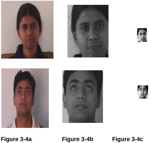
This phase involved the acquisition of standard face image database from AT &T Database [11](10 images for each of the 40 distinct face images) and Indian Face Database[11](10 images for each of the 60 distinct face images) through the Internet and the pre-processing of such images using MATLAB. The pre-processed images were categorised into Dataset1, Dataset2, and Dataset3. Again, every dataset contained probe database and train database. The train database contained images assumed to be known whereas unknown (test) images are contained in the probe database. The datasets varied based on the number of images per person in its train database. Thus, Dataset1, 2, and 3 contained 3, 5, and 10 images per person respectively. The probe database is one image per person selected from the corresponding train database. Figures 3-4 and 3-5 below were samples of face images from Indian Face Database and AT& T Face Image Database respectively used to experiment the algorithms.

Figure 3-4a Figure 3-4b Figure 3-4c

(3)

Figure 3-5 a Figure 3-5b Figure 3-5c

Figure a=Original Images (112x92 pixels), Figure b =Resized images (60x50 pixels), Figure c=Histogram equalised Images

3.2 Training Phase

In this phase, the PCA and LDA algorithms were used to first and foremost convert each face image in a train database into image vector to form training set. Feature vectors were then extracted and stored. Below were the algorithms used; PCA Algorithm

 Convert each image (60x50) to image vector 3000x1(x)  Form training set of image vectors

 Find mean vector of all image vectors, m  Compute mean-centeredmatrix, A=x-m  Compute covariance matrix,L=A.AT

 Find eigenvectors and corresponding eigenvalues of covariance matrix, eig(L)

 Select eigenvectors with eigenvalues greater than zero, ek

 Compute eigenface, w=A. ek

 Find projected eigenface, Ω= w‘.A

LDA Algorithm

 Use projected eigenface space of PCA  Mean of each class of eigenface  Overall mean of eigenface  compute within scatter matrix, Sw  Compute between scatter matrix, Sb

 Find eigenvectors and eigenvalues using matlab function eig(sb,sw)

 Sort, and select eigenvectors with eigenvalues greater than zero (fk)

 Find fisherface, w=fk..Projected eigenface

 Find projected fisherface, Ω= w‘.projected eigenface

3.3 Recognition Phase

At this stage, probe /test image was selected and used as input image to initiate the recognition process. Here

determination was made whether input image was similar to any of the images (or has a match) in the training set using the similarity measure.

Recognition Algorithm

 Convert the probe/test image to image vector  Subtract overall mean vector from image vector  Project mean centered image vector onto

eigenface/fisherface

 Use any of the similarity measure to compare projected eigenface /fisherface of training set and probe test  Minimum value (for Euclidean or City Block) or maximum

cosine value indicates a match.

Each of the six projection-metric methods(PCA-Euclidean, PCA-City Block, PCA- Cosine, LDA-Euclidean, LDA-City Block and LDA-Cosine) was tested with all the three datasets of each database.

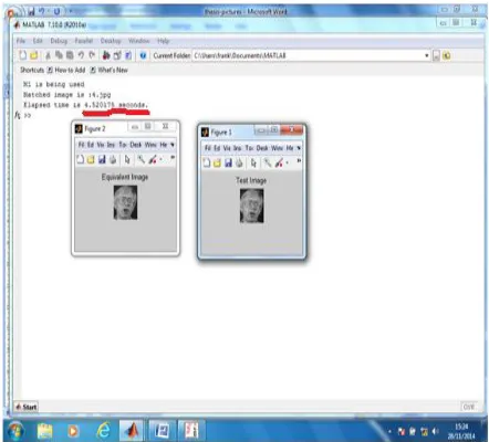
Figure 3-13: A sample of results of Indian Face tested

Figure 3-14: A sample of results of AT& T face image tested.

(4)

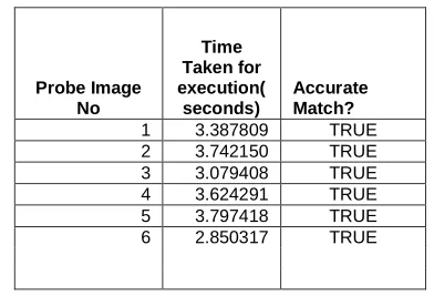
289 TABLE 3-1: PCA-Euclidean Distance Metric with AT & T

Database (ORCL)

A. dataset1:( TrainDatabase1 and ProbeDatabase1)

Probe Image No Time Taken for execution( seconds) Accurate Match? 1 3.387809 TRUE 2 3.742150 TRUE 3 3.079408 TRUE 4 3.624291 TRUE 5 3.797418 TRUE 6 2.850317 TRUE

B. dataset2: (TrainDatabase2 and ProbeDatabase2)

Probe Image No

Time Taken for execution(seconds)

Accurate Match?

1 6.199392 TRUE

2 4.882568 TRUE

3 4.005939 TRUE

4 4.229203 TRUE

5 4.22299 TRUE

6 4.289686 TRUE

C. dataset 3:( TrainDatabase3 and ProbeDatabase3)

Probe Image No

Time Taken for execution(seconds)

Accurate Match?

1 10.747025 TRUE

2 10.217329 TRUE

3 10.83966 TRUE

4 11.809159 TRUE

5 10.464620 TRUE

6 10.547158 TRUE

Table 3-1: A sample of projection-metric table recording time of execution and accuracy of each algorithm M1 in the figures indicated the Similarity metric used which (in these figures)was Euclidean Distance. In the situation where M2(City Block) or M3(Cosine) was used as similarity metric M2 or M3 was shown instead of M1.

3.4 Performance evaluation phase: This phase showed the comparative analysis of the outcome of face recognition techniques employed. This was based on the accuracy (number of correct match), time of execution of algorithm. The generalization ability of the combined projection-metric methods was also ascertained.The generalization ability of an algorithm has several meanings some of which are; It is an ability to maintain a recognition rate when reducing the number of images in the training set [6]. Alternatively, when considering the algorithms that use more than one image per

class in the training database, the ability of an algorithm to maintain a recognition rate when the number of images per class used in training is reduced [8].

4.0 ANALYSIS OF RESULTS

The implementation of the six projection-metric methods with all the datasets proved to have 100% accurate recognition rate as illustrated in Tables 4-1 and 4-2. They also proved to have excellent generalization ability in that each maintained its recognition rate when the analysis in Table 4-1 and 4-2 was observed from the dataset 3 followed by dataset2 and then dataset1 for the two databases.

Table 4-1: Accurate recognition rate for execution of projection-metric algorithm with AT&T database

AT &T Database

Dataset 1 Dataset 2 Dataset 3

PROJECTIO

N-/METRIC A B C A B C

A B C

PCA-M1 40

4 0 100 % 4 0 4 0 100 % 4 0 4 0 100 %

PCA-M2 40

4 0 100 % 4 0 4 0 100 % 4 0 4 0 100 %

PCA-M3 40

4 0 100 % 4 0 4 0 100 % 4 0 4 0 100 %

LDA-M1 40

4 0 100 % 4 0 4 0 100 % 4 0 4 0 100 %

LDA-M2 40

4 0 100 % 4 0 4 0 100 % 4 0 4 0 100 %

LDA-M3 40 4 0 100 % 4 0 4 0 100 % 4 0 4 0 100 %

M1-Euclidean Distance Metric M2-City Block Metric M3-Cosine Metric

A=Number of Correctly Matched Images,B= Number of Probe/Test Images,

C=Recognition Rate =A/B*100%

TABLE 4-2: Accurate recognition rate for execution of projection-metric algorithm with Indian Facedatabase

INDIAN FACE DATABASE

Dataset 1 Dataset 2 Dataset 3

PROJECTION

-/METRIC A B C A B C

A B C

(5)

LDA-M1

5 0

100 %

5 0

100 %

5 0

100 %

LDA-M2

5 0

100 %

5 0

100 %

5 0

100 %

LDA-M3 5 0

5 0

100 %

5 0

100 %

5 0

100 %

A=Number of Correctly Matched Images,B= Number of Probe/Test Images,

C=Recognition Rate =A/B*100%

The Tables 4-3 and 4-4 below showed the average time of execution of each algorithm‘s time of recognising all the individual images in a probe database of a particular dataset. That is, the individual times (in seconds) recorded for a particular projection-metric algorithm for recognising individualtest images of a probe database in a particular dataset were summed up and divided by the number of test images of the probe database in the particular dataset being.

TABLE 4-3: Average Execution Time (in seconds) For Projection-Metric Algorithms with AT& T Database

TABLE 4-4: Average Execution Time (in seconds) For Projection-Metric Algorithms with Indian Face Database

M1-Euclidean Distance Metric M2-City Block Metric M3-Cosine Metric

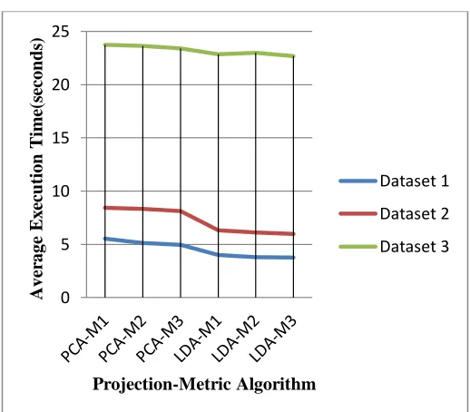
Figure 4-2: Average Execution Time (in seconds) For Projection-Metric Algorithms with AT & T Database

Figure 4-2 is a graphical representation of Table 4-3

Figure 4-4: Average Execution (in seconds) for Projection-Metric Algorithms with Indian Face Database

Figure 4-4 is graphical representation of the Table 4-4

The overall ranking of the projection-metric table 4-6 below was done based on projection-metric algorithm‘s average execution time when a particular Dataset was used. This was obtained from Table 4-3 and 4-4. The rankings of each projection metric across all datasets of the two databases were averaged and the minimum average ranking became the most efficient while the maximum was the least efficient in the recognition of probe/test face image.

0 2 4 6 8 10 12

PC

A-M

1

PC

A-M

2

PC

A-M

3

LD

A-M

1

LDA-M2

LD

A-M

3

Ave

rage

E

x

ec

u

tion

T

im

e

Projection-Metric Algorithm

Dataset 1

Dataset 2

Dataset 3

0 5 10 15 20 25

Ave

rage

E

x

ec

u

tion

T

im

e(

se

con

d

s)

Projection-Metric Algorithm

Dataset 1

Dataset 2

Dataset 3 ALGORITHMS

AVERAGE EXECUTION TIME(SECONDS)

Projection-Metric

Dataset 1

Dataset

2 Dataset 3

PCA-M1 3.20 4.44 10.62

PCA-M2 3.20 4.52 10.89

PCA-M3 3.07 4.48 10.71

LDA-M1 2.59 3.52 8.69

LDA-M2 2.58 3.44 9.28

LDA-M3 2.57 3.56 8.57

ALGORITHM

AVERAGE EXECUTION TIME (SECONDS)

Projection-Metric Dataset 1 Dataset 2

Dataset 3

PCA-M1 5.54 8.42 23.73

PCA-M2 5.12 8.32 23.62

PCA-M3 4.96 8.12 23.4

LDA-M1 3.99 6.31 22.85

LDA-M2 3.81 6.11 23

(6)

291 Table 4-6: OVERALL RANKING OF THE

PROJECTION-METRICS

The figures4-2 and 4-4 indicated that all the LDA projection methods were more efficient in terms of average time of execution than the PCA for all the datasets tested. The overall ranking of projection metrics showed that LDA-Cosine Metric was the most efficient among all the projection-metric methods implemented and has the ability to withstand increased data size since even with dataset3 it still ranked first as illustrated in Table 4-6.

5.0 CONCLUSION

In conclusion, the study was able to prove that the recognition rate and generalization abilities of all the projection-metrics considered were excellently effective. Besides the fact that LDA outperformed PCA in the study, LDA-Cosine metric method was not only efficient but could withstand the larger training database. It therefore means that in a situation where time is of essence and data size is large or is likely to increase over time the appropriate projection-metric method to be recommended is LDA-Cosine metric method.

FUTURE WORK

Future work will be to consider other similarity matching metrics like Thurstone-Shepard Model, Mahalanobis distance and others in addition to the three used and larger training data size.

ACKNOWLEDGEMENT

Standard face image database from AT & T Laboratories at Cambridge and Indian Institute of Technology, Kanpur were used for experiments. Mr Amir Hossein Omidvarmia, whose MATLAB sample codes on the Internet greatly helped me in my work.

REFERENCES

[1] Abhijit Kulshrestha, Raj Kumar Sahu, Yash Pal Singh ―A Comparative Study of Face Recognition System Using PCA and LDA‖ , International Journal of IT, Engineering and Applied Sciences Research (IJIEASR) ISSN: 2319-4413 Volume 2, No. 10, October 2013

[2] J. R. Beveridge, K. She B. Draper & G. H. Givens. ―Anonparametric Statistical Comparison& Linear Discriminant Subsapces for face recognition‖ in Proc of the IEEE Conference on Computer Vision & Pattern Recognition, CVPR‘01, Kauai, 2001, PP.535-542

[3] Keyur Brahmbhatt, Premal J Patel, Samip A Patel,Udesang K Jaliya ―A Comparative Study of PCA & LDA Human Face Recognition Methods‖, National Conference on Recent Trends in Engineering & Technology, 13-14 May 2011 B.V.M. Engineering College, V.V.Nagar,Gujarat,India.

[4] Kresimir Delac , Mislav Grgic and Sonja Grgic, ―Generalization Abilities of Appearance-Based SubspaceFace Recognition Algorithms‖ 12th Int. Workshop on Systems, Signals & Image Processing, 22-24 September 2005

[5] Kresimir Delac , Mislav Grgic and Sonja Grgic ― Independent Comparative Study of PCA, ICA AND LDA on the FERET Data set‖

[7] M. Turk and A. Pentland, Eigenfaces for recognition‖, Journal of Cognitive Neuroscience. Vol.3 no.1, PP76-86, 1991

[8] Navarrete, P., Ruiz-del-Solar, J. (2002) ‗Analysis and Comparison of Eigenspace-Based Face Recognition Approaches‘, International Journal of Pattern Recognition and Artificial Intelligence, Vol.16, No.7, pp. 817-830, November.

[9] Nikola Paveˇsi´c,and Vitomir ˇStruc ―A comparative assessment of appearance based feature extraction techniques and their susceptibility to image degradations in face recognition systems‖, Member, IEEE Aeordia Univesooo

[10]P.N. Belhumeur, J.P. Hespanha andD.J. Kriegman‖ Eigenfaces vs.Fisherfaces: recognition using class specific linear projection,‖ in Proc. Ofthe 4th European Conference on Computer Vision, ECCV‘96, Cambridge, UK, 1996, pp. 45-58.