www.nat-hazards-earth-syst-sci.net/11/2047/2011/ doi:10.5194/nhess-11-2047-2011
© Author(s) 2011. CC Attribution 3.0 License.
and Earth
System Sciences
The application of numerical debris flow modelling for the
generation of physical vulnerability curves
B. Quan Luna1, J. Blahut2, C. J. van Westen1, S. Sterlacchini3, T. W. J. van Asch4, and S. O. Akbas5 1Faculty of Geoinformation Science and Earth Observation (ITC), University of Twente, P.O. Box 6, 7500 AA Enschede, The Netherlands
2Institute of Rock Structure and Mechanics, Academy of Sciences of the Czech Republic, V Holeˇsovi˘ck´ach 41, 182 09 Prague, Czech Republic
3Institute for the Dynamic Environmental Processes, National Research Council (CNR-IDPA), Piazza della Scienza 1, 20126 Milan, Italy
4Faculty of Geosciences, Utrecht University, Utrecht, The Netherlands 5Civil Engineering Department, Gazi University, Ankara, Turkey
Received: 24 September 2010 – Revised: 7 March 2011 – Accepted: 2 April 2011 – Published: 25 July 2011
Abstract. For a quantitative assessment of debris flow risk, it is essential to consider not only the hazardous process itself but also to perform an analysis of its consequences. This should include the estimation of the expected monetary losses as the product of the hazard with a given magnitude and the vulnerability of the elements exposed. A quantifi-able integrated approach of both hazard and vulnerability is becoming a required practice in risk reduction management. This study aims at developing physical vulnerability curves for debris flows through the use of a dynamic run-out model. Dynamic run-out models for debris flows are able to calcu-late physical outputs (extension, depths, velocities, impact pressures) and to determine the zones where the elements at risk could suffer an impact. These results can then be applied to consequence analyses and risk calculations. On 13 July 2008, after more than two days of intense rainfall, several debris and mud flows were released in the central part of the Valtellina Valley (Lombardy Region, Northern Italy). One of the largest debris flows events occurred in a village called Selvetta. The debris flow event was reconstructed af-ter extensive field work and inaf-terviews with local inhabitants and civil protection teams. The Selvetta event was modelled with the FLO-2D program, an Eulerian formulation with a finite differences numerical scheme that requires the spec-ification of an input hydrograph. The internal stresses are isotropic and the basal shear stresses are calculated using a quadratic model. The behaviour and run-out of the flow was reconstructed. The significance of calculated values of the flow depth, velocity, and pressure were investigated in terms
Correspondence to: B. Quan Luna
of the resulting damage to the affected buildings. The physi-cal damage was quantified for each affected structure within the context of physical vulnerability, which was calculated as the ratio between the monetary loss and the reconstruction value. Three different empirical vulnerability curves were obtained, which are functions of debris flow depth, impact pressure, and kinematic viscosity, respectively. A quantita-tive approach to estimate the vulnerability of an exposed el-ement to a debris flow which can be independent of the tem-poral occurrence of the hazard event is presented.
1 Introduction
2048 B. Quan Luna et al.: The application of numerical debris flow modelling In order to improve the results of a debris flow risk
as-sessment, it is necessary to analyze the hazard event using quantitative information in every step of the process (van Asch et al., 2007) and the vulnerability of the elements ex-posed. The contribution of the dynamic run-out models in-side a quantitative assessment is to reproduce the distribution of the material along the course, its intensity, and the zone where the elements will experience an impact. For this rea-son, dynamic run-out models have been used in recent years as a tool that links the outputs of a debris flow hazard initia-tion/susceptibility modelling (released volumes) with physi-cal vulnerability curves.
1.1 Numerical modelling for hazard analysis in a Quantitative Risk Assessment (QRA)
Different approaches and methods have been developed in the past for a quantitative risk analysis using dynamic run-out models and where the vulnerability of the elements at risk is described in a quantitative or qualitative manner. In this direction, Bell and Glade (2004) performed a quanti-tative risk analysis (focusing on the risks to life) in NW-Iceland for debris flows and rock falls. Their approach to the hazards is based on empirical and process modelling that resulted in specific run-out maps. The hazard zones were de-termined based on the recurrence interval of the respective processes. For the determination of the respective levels of vulnerability, a semi-quantitative approach defined by matri-ces was used based on available literature and the authors’ past findings (Glade, 2004). Their calculated vulnerability levels were incorporated into a consequence analysis that in-cluded the definition of elements at risk, the determination of spatial and temporal probabilities of impact, and the seasonal occurrence of the event. Calvo and Savi (2008) proposed a method for a risk analysis in a debris flow-prone area in Ar-denno (Italian Alps), utilizing a Monte Carlo procedure to obtain synthetic samples of debris flows. To simulate the propagation of the debris flow on the alluvial fan, the FLO-2D model (O’Brien et al., 1993) was applied and probability density functions of the outputs of a model (forces) were ob-tained. Three different vulnerability functions were adopted to examine their effect on risk maps. Muir et al. (2008) pre-sented a case study of quantitative risk assessment to a site-specific natural terrain in Hong Kong, where various scenar-ios were generated with different source volumes and sets of rheological parameters derived from the back analyses of natural terrain landslides in Hong Kong. Debris mobility modelling was performed using the Debris Mobility Model (DMM) software developed by the Geotechnical Engineer-ing Office (Kwan and Sun, 2006), which is an extension of Hungr’s (1995) DAN model. They derived probability dis-tributions from past events run-outs and calculated the prob-ability distribution of debris mobility for each volume class. Regarding the vulnerability, they used an “Overall
mitigation action was introduced. A cost-benefit analysis of each scenario was performed considering the direct effect on human life, houses, and lifelines.
The recent work done by means of numerical physical modelling within a risk analysis suggests that dynamic run-out models (correctly used) can be of practical assistance when attempting to quantify the assessment. Together with a good understanding of the slope processes and their rela-tionship with other conditional factors, run-out models re-sults can be used in a hazard analysis to: estimate the spa-tial probability of the flow affecting a certain place with de-tailed outputs as deposition patterns, travelled distance and path, and velocities and impact pressures. Results obtained from the run-out modelling are directly involved as factors that influence and affect the vulnerability of an exposed el-ement. However, quantitative vulnerability information for landslides is difficult to obtain due to the large variability in landslides types, the difficulty in quantifying landslides magnitude, and the lack of substantial historical damage databases (van Westen et al., 2006; Douglas, 2007).
1.2 Physical vulnerability assessment
Several efforts have been made in the past to define and as-sess the vulnerability of an element or group of elements ex-posed to a landslide hazard. The vulnerability can be classi-fied as: physical, functional, and systemic vulnerability. The
physical vulnerability relates to the consequences or the
re-sults of an impact of a landslide on an element (Glade, 2003).
Functional vulnerability depends on the damage level of the
element at risk and its ability to keep functioning after an event (Leone et al., 1996). Systemic vulnerability defines the level of damage between the interconnections and functional-ity of the elements exposed to a hazard (Pascale et al., 2010). In this paper, a focus on the physical vulnerability will be highlighted with regard to a method which is commonly used in a quantitative risk assessment.
In a quantitative risk assessment, physical vulnerability is commonly expressed as the degree of loss or damage to a given element within the area affected by the hazard. It is a conditional probability, given that a landslide with a cer-tain magnitude occurs and the element at risk is on or in the path of the landslide. Physical vulnerability is a represen-tation of the expected level of damage and is quantified on a scale of 0 (no loss or damage) to 1 (total loss or damage) (Fell et al., 2005). Thus, vulnerability assessment requires an understanding of the interaction between the hazard event and the exposed element. This interaction can be expressed by damage or vulnerability curves.
Some progress has been made in developing vulnerabil-ity curves, matrices, and functions for several types of haz-ards and mass movements. Extensive work has been carried out by FEMA (Federal Emergency Management Agency) on vulnerability functions for earthquakes, floods, and hur-ricanes. These functions are used in the HAZUS (Hazard
US) software application to quantitatively estimate the losses in terms of direct costs (e.g. repair, loss of functionality), as well as regional economic impact and casualties (Hazus, 2006). In the case of snow avalanches, Wilhelm (1998) ob-tained a function by analysing the damages caused in terms of impact pressure by dense snow avalanches on concrete buildings with reinforcement. The building vulnerability was defined as the ratio of the cost of repairing the damages and the value of the building. Based on the function proposed by Wilhelm (1998), Cappiabanca et al. (2006) developed a func-tion for people inside the buildings. Using the same approach of relating the expected losses of a structure with the impact pressures of the avalanche, Barbolini et al. (2004) proposed vulnerability functions for buildings and persons for powder snow events. To overcome the scarcity of well documented events and their consequences, Bertrand et al. (2010) used numerical models to simulate the structure behaviour under snow avalanche loading. The structures were modelled in three dimensions with a finite element method (FEM), and a damage index was defined on global and local parameters of the buildings (e.g. geometry of the structure, compressive strength of the concrete). The vulnerability was established as a function of the impact pressure and the structure fea-tures. For rock falls, Heinimann (1999) estimated vulnera-bility curves as damage functions of six different categories (type) of buildings related to the intensity of the rock fall. The response of reinforced concrete buildings to rock fall impact was investigated by Mavrouli and Corominas (2010), considering a single hit on the basement columns. They cal-culated for a range of rock fall paths and intensities, a damage index (DI) defined as the ratio of structural elements that fail to the total number of structural elements.
2050 B. Quan Luna et al.: The application of numerical debris flow modelling a well-documented debris flow event in the Austrian Alps to
derive a vulnerability function for brick masonry and con-crete buildings. They defined a damage ratio that describes the amount of damage related to the overall damage poten-tial of the structure. A vulnerability function was created from the calculated damage ratio and the debris flow inten-sity (flow height). A comprehensive review of several qual-itative vulnerability methods used in landslide risk analysis was made by Glade (2003).
Whereas the above mentioned examples analyze the haz-ard separately from the vulnerability of the elements at risk, our aim is to use the strength of the debris flow run-out mod-els to quantify physical vulnerability by means of the impact pressure outputs. We present an integrated approach of de-tailed rainfall data and dynamic modelling to calculate the in-tensity and run-out zone of the 2008 Selvetta debris flow that caused damage to thirteen buildings. The debris flow event was reconstructed and back-analyzed. Geomorphologic in-vestigations were carried out to study the behaviour of the flow and intensity aspects such as run-out distances, veloci-ties, and depths. Synthetic physical vulnerability curves were prepared based on the flow depth, impact pressures, and kine-matic viscosity. These curves relate the physical outputs of the modelling and the economic values of the elements at risk.
2 Selvetta study site and past events in the region
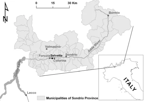
The Selvetta study site is situated inside the Valtellina Valley in the Italian Central Alps (Fig. 1) and administratively is a part of the Colorina municipality. Geomorphologically, it be-longs to the Orobic Alps which are forming the north-facing slopes of the Valtellina Valley (a U-shaped valley profile de-rived from Quaternary glacial activity). Selvetta is located in a north-facing slope of the valley. The slopes are mainly composed of metamorphic rocks (gneiss, mica schist, phyl-lite, and quartzite) and intrusive rock units, with subordinate sedimentary rocks (Crosta et al., 2003). On less steep parts, two Pleistocene glacial terraces could be distinguished at the height of about 560–760 m a.s.l. and 1120–1240 m a.s.l. The lower sections are covered with glacial, fluvio-glacial, and colluvial deposits of variable thickness.
Valtellina Valley is an active region with respect to ge-omorphologic processes and mass movements. In the re-cent past, the valley has suffered from major catastrophic events in terms of flooding and landslides. In May 1983, heavy precipitations triggered more than 200 shallow land-slides and debris flows in Valtellina. A cumulated precipita-tion of 453 mm was measured during the month, which cor-responds to 34% of the total annual precipitation. Landslides happened mainly on vine-terraced slopes and most of the landslides started on slopes between 30◦and 40◦. Three soil-slips evolved into larger debris flows with lengths from 300 to 460 m and areas reaching 60 000 m2, causing 14 casualties
10 Figures and Tables
900 901 902 903 904 905
906 907 908 909
910 Figure 1
22
Fig. 1. Location of the Selvetta case study area.
(Cancelli and Nova, 1985). In July 1987, more than 500 mass movements were triggered by a severe rain storm (Crosta et al., 1990). Five villages and the transportation infrastruc-ture were critically damaged. A total of 25 000 evacuated persons, 53 casualties and 2000 million euros ( C) of dam-ages were recorded (Luino, 2005). From 14 to 17 Novem-ber 2000, prolonged and intense rainfalls triggered about 260 shallow landslides in Valtellina (Crosta et al., 2003). About 200 soil slips and slumps took place in the terraced slopes, and one third of them evolved into debris flows (Chen et al., 2006). In November 2002, the Valtellina area was affected by an extreme rainfall (more than 700 mm) that triggered more than 70 soil slips and debris flows. The event caused 2 ca-sualties and extensive damages to structures and economic activities, evaluated in 500 millions of euros (Aleotti et al., 2004).
3 The Selvetta 2008 debris flow
The largest muddy-debris flow occurred in the village of Selvetta. According to the morphological classification of debris flows for the South-Central Alps proposed by Crosta et al. (1990), this debris flow can be classified as a debris avalanche evolving into channelled debris flow. The debris flow event was reconstructed after extensive field work and interviews with local inhabitants and civil protection teams. At first, several rock blocks of a size up to 2 m3fell down from the direction of a small torrent above the village. The blocks were followed by a first surge of debris and mud that damaged the houses. This surge caused the most dam-age in the deposition area. This was followed by a second hyperconcentrated flow with fine mud content that partially washed away the accumulation from the first wave.
The main objective of the fieldwork was to collect in-formation to describe the behaviour of the flow during its course. Measurements of the flow depths along the path and sedimentation features that hinted the evolution of the flow were carried out. Entrainment and deposition features were mapped. The deposits inside and outside of the channel were considered and channel profiles were made in locations where the velocities and discharge of the flow could be de-duced.
The evolution of the flow in terms of velocity was recon-structed by the use of empirical formulas. The estimation of the velocity is important to evaluate the flow behaviour and assess its rheology. To derive the mean flow velocity in each channel cross-section, the superelevation formula (Eq. 1) proposed by McClung (2001) and Prochaska et al. (2008) was applied:
v=
r Rcg
k 1h
b (1)
where,vis the mean velocity of the flow (m s−1),Rcis the channel’s radius curvature (m),gis the gravity acceleration (m s−2),1h is the superelevation height (m),k is a correc-tion factor for the viscosity, and b is the flow width (m). Hungr (2007) in Prochaska et al. (2008) indicated that the value of the correction factor can be usually “1”, with the ex-ception of cases with sharp bends where some shock waves develop.
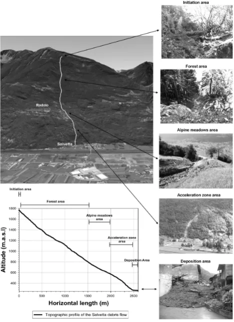
Geomorphologic investigations allowed distinguishing the following five main sections of the flow: (1) the proper scarp, (2) path in forested area, (3) path on alpine mead-ows, (4) accelerating section, and (5) accumulation area (Fig. 2).
The initiation area of the flow was situated approximately at 1760 m a.s.l. in a coniferous forest. The proper scarp was very small, with an area of about 20 m2and a height about 0.5 m. The debris flow originated as a soil-slip in thin collu-vial cover on a very steep (>45◦) forested slope. This sug-gests that the flow started as a small failure and gained mo-mentum with additional entrained material from the channel bed and walls. Another important source for the increase
911 912 913
914 Figure 2
23
Fig. 2. Google image and profile of the Selvetta debris flow path
with the five main morphological sections determined on the field.
2052 B. Quan Luna et al.: The application of numerical debris flow modelling
915 916
917 918 919 920 921 922 923 924 925 926 927 928 929
Figure 3
24
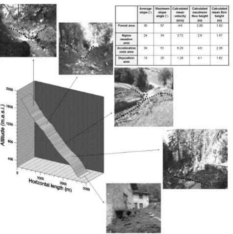
Fig. 3. Selvetta debris flow path including the calculated mean
ve-locity, maximum flow height, and mean flow height for each mor-phologic section.
sorting and the angle of rest in the borders of the final de-posit. Deposits consisted of a fine-grained fluid mixture with suspended coarse debris on the top and fine material on the bottom.
Precipitation records showed that the flow did not occur immediately after the peak precipitation which was recorded at 7 a.m., but with more than three hour delay. Unfortunately, there is no rain gauge in the proximity of the initiation zone. The closest one is in Morbegno (about 8 km from the scarp) and shows hourly peak rainfall of 22 mm h−1between 6 and 7 a.m. (Fig. 4). The cumulated rainfall during 48 h before the event reached 92 mm. Although this record did not precisely describe the situation in the initiation area, it could be used for a rough estimation of precipitation and for measuring the delay of initiation after peak precipitation, because records from other gauges in the vicinity also show the rainfall peak between 6 and 7 a.m.
One of the main characteristics of the event is the influence of the entrainment process on the flow. The channel experi-enced considerable deepening and bank erosion. In several parts of the channel, it was found that obstruction by large boulders and trees may have temporarily influenced the flow behaviour by causing a dam-break effect that resulted in the two different surges in the deposition area.
There are 95 buildings situated in Selvetta. The debris flow event destroyed two of them and caused damage of varying levels of severity to another eleven buildings. Structural dam-age was reported to the facilities located on the alluvial fan (roads). Also, a lot of damage was reported for cars and
agri-930 931
932 933
Figure 4
934
935
25
Fig. 4. Derived hydrograph of the debris flow, including the
re-leased volume and peak discharge (above) obtained from the hourly precipitation records from the Morbegno rain gauge (bottom).
cultural machinery. Fortunately, no victims or injuries were reported, mainly because of the awareness of the civil de-fence organization who evacuated the local inhabitants from their houses.
4 Modelling of the event for determining vulnerability curves
936 937 938 939
Figure 5
26
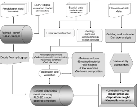
Fig. 5. Flowchart of the methodology applied in the Selvetta case
study area.
The mathematical model used to model the Selvetta de-bris flow event was FLO-2D, which is an Eulerian two-dimensional finite difference model that is able to route non-Newtonian flows in a complex topography based on a volume-conservation model. The model input is in the form of a flow hydrograph at the head of a depositional debris fan, distributing the debris over the fan surface, allowing for ob-structions and pathways such as infrastructures (buildings, roads, channels, and bridges). These make the model rele-vant for the determination of flow patterns on the surface of a fan. The flow volume is routed through a series of tiles that simulates overland flow (2-D flow), or through line segments for channel routing (1-D flow). Flow in two dimensions is accomplished through a numerical integration of the equa-tions of motion and the conservation of fluid volume. The governing equations are originally presented by O’Brien et al. (1993).
The FLO-2D software models the shear stress as a sum-mation of five shear stress components: the cohesive yield stress, the Mohr-Coulomb shear, the viscous shear stress, the turbulent shear stress, and the dispersive shear stress. All these components can be written in terms of shear rates giv-ing a quadratic rheological model function of sediment con-centration. The depth-integrated rheology is expressed (after dividing the shear stresses by the hydrostatic pressure at the bottom of the flowγmh)as Eq. (2):
Sf= τy
γmh
+ KηV
8γmh2+ n2tdV2
h4/3 (2)
where,Sf is the friction slope (equal to the shear stress di-vided byγmh);V is the depth-averaged velocity; τy andη are the yield stress and viscosity of the fluid, respectively, which are both a function of the sediment concentration by volume;γmis the specific weight of the fluid matrix;Kis a
dimensionless resistance parameter that equals 24 for lami-nar flow in smooth, wide, rectangular channels, but increases with roughness and irregular cross section geometry; and ntd is an empirically modified Manningnvalue that takes into account the turbulent and dispersive (inertial grain shear) components of flow resistance. The parametersτyandηare defined as exponential functions of sediment concentration which may vary over time. The yield stress (Eq. 3) and the viscosity (Eq. 4) are calculated as follows:
τy=α1eβ1Cv (3)
η=α2eβ2Cv (4)
where,α1,β1,α2,andβ2are regression constants obtained from the correlation of results of laboratory experiments,Cv is the fine sediment concentration (silt- and clay-size parti-cles) by volume (FLO-2D, 2009)
The boundary conditions are specified as follows: the in-flow condition is defined in one or more upstream grid ele-ments with a hydrograph (water discharge vs. time) and val-ues ofCvfor each point in the hydrograph. The outflow con-dition is specified in one or more downstream grid elements. The model requires the specification of the terrain surface as a uniformly spaced grid. Within the terrain surface grid, a computational grid, i.e. a domain for the calculations, must be specified. The Manning n value should be assigned to each grid element to account for the hydraulic roughness of the terrain surface. The values can be spatially variable to account for differences in surface coverage (FLO-2D, 2009). 4.1 Rainfall modelling
2054 B. Quan Luna et al.: The application of numerical debris flow modelling 4.2 Debris flow modelling
The estimation of the peak discharge inside the discharge hy-drograph is of vital importance as it determines the maximum velocity and flow depth, momentum, impact forces, ability to overrun channel walls, as well as the run-out distance (Rick-enmann, 1999; Whipple, 1992; Chen et al., 2007). For the estimation of the final debris flow hydrograph, the volumes of the entrained material estimated from measurements dur-ing the field work were introduced as an additional and vari-able sediment concentration into the hydrographs used in the FLO-2D model with the empirical formula use proposed by Mizuyama et al. (1992), who proposed a relation between the magnitude of the debris flow (volume in m3)and the peak discharge for muddy-debris flow (Eq. 5):
Qp=0.0188M0.790 (5)
where, Qp is the peak discharge (in m3s−1) andM is the debris flow volume magnitude (in m3). A time-stage of sed-iment concentration was produced based on the shape of the hydrograph (Fig. 5). This was done to agree with observa-tions that the peaks in debris flow hydrographs correspond to high sediment concentrations, while the final part of the hydrograph have a more diluted composition. The procedure also reproduced the distribution of sediment concentration influenced by a dilution in the falling tail of the hydrograph. The maximum and minimum concentrations were 0.55 and 0.25, respectively.
Parameterization of the FLO-2D model was done by cali-bration, since no independent estimates of the model friction parameters were available. The calibration of the model was based on a trial-and-error selection of rheological models and parameters, and the adjustment of the input parameters which define the flow resistance. Parameters were adjusted until good agreement between the simulated and observed characteristics were accomplished with the following crite-ria: (i) velocity and height of the debris flow along the chan-nel, (ii) final run-out, and (iii) accumulation pattern in the de-position area. The parameters that reasonably filled the cali-bration criteria and had the best results wereτy= 950 Pa and η= 1500 Pa. These rheological parameters were calculated according to the sediment concentration of the flow (taken into account inside the debris flow hydrograph) and the con-stant values of α= 0.0345 for τy and 0.00283 for η; and
ß = 20.1 forτy and 23.0 forη were selected from O’Brien and Julien (1988). The chosen Manning n-values that charac-terize the roughness of the terrain were = 0.04 s m−1/3where the flow was channelled, and 0.15 s m−1/3in the deposition zone. The Manning n-values and the constant value along the channel ofK=24 were selected as suggested in the FLO-2D manual.
Figure 6 shows the maximum run-out and deposition mod-elled by FLO-2D and the field-measured extent of the event which underlines the good agreement of the simulation with
940
941 Figure 6
27
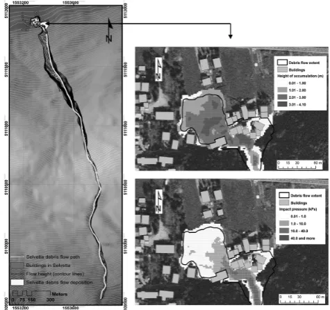
Fig. 6. Modelling results of the Selvetta debris flow (left).
Com-parison of the real and modelled debris flow run-out extent: The maximum heights of the accumulation and maximum impact pres-sures modelled by the FLO-2D model are shown (right).
what actually happened. The modelled heights of accumula-tion show good agreement with the real situaaccumula-tion measured in the field. The highest accumulations are reached upslope from the destroyed and heavily damaged buildings, decreas-ing to the edges of the deposition area. It should be noted that in some cases the flow did not reach some of the lightly damaged structures. This is caused by the fact that FLO-2D does not model the destruction of the building and thus it remains as an obstacle causing the “shadow” effect. Appar-ent increase of heights of accumulation in the distal parts of the flow is most probably caused by imprecision in the used DEM. Highest values of impact pressure are reached imme-diately near the start of the apex. Afterwards, the pressures continuously decrease. This is caused by the progressive de-crease of accumulation heights and velocities on the alluvial fan.
5 Generation of vulnerability curves
5.1 Methodology
In our approach, the vulnerability functions were calculated using damage data obtained from the official documents of damage assessment coupled with the information from the modelling outputs. This approach allows calculation of vul-nerability functions using the height of debris accumulation and also the impact pressure. The impact pressure informa-tion is widely used in snow avalanche risk assessment but it is not widely applied for debris flows risk calculations.
The damage data was analyzed from the RASDA doc-uments (RAccolta Scheda DAnni – Damage Assessment Form), which are mandatory to be drafted within 48 h af-ter a disasaf-ter for claiming recompensation funding. For the Selvetta debris flow, these documents were prepared by the engineers of the General Directorate of Civil Protection of the Lombardy Region and the local police, where they esti-mated the losses in monetary values of each building. For each building, the approximate reconstruction value was cal-culated according to building type and size, using the data given in the Housing Prices Index prepared by the Engineers and Architects of Milan (DEI, 2006). All of the buildings were single to three storey brick masonry and concrete struc-tures. The calculated reconstruction values of the buildings in the studied area ranged from C 66 000 to C 455 000; while the recorded damage ranged from about C 2000 to C 290 000 (Table 1).
Vulnerability is defined by the fraction between the loss and the individual reconstruction value, and was calculated for each of the thirteen building structures that were affected by the debris flow event (Fig. 7). The obtained results were consequently coupled with the modelling results (height of accumulation, impact pressures). This allows developing vulnerability curves that relate the building vulnerability val-ues with the process intensity. The generated physical vul-nerability curves can be used as an approach for the esti-mation of the structural resistance of buildings affected by a debris flow event.
5.2 Vulnerability curve using heights of accumulation
Height of accumulation values were extracted for each af-fected building. For every building the maximum and mini-mum heights of accumulation varied a lot. As a consequence, an average height near building walls oriented towards the flow direction was considered. Figure 8 shows the relation-ship between the vulnerability and deposition height values.
Figure 8 indicates that the vulnerability increases with in-creasing deposition height. We propose to use a logistic func-tion (Eq. 6). The calculated funcfunc-tion has coefficient of deter-mination (r2)is 0.99, for intensities between 0 and 3.63 m:
v= 1.49×|h/2.513| |−1.938|
1+|h/2.513||−1.938| forh≤3.63 m
v=1 forh >3.63 m
(6)
where, V is vulnerability and h is the modelled height of accumulation. From its definition the vulnerability cannot exceed 1, thus for intensities higher than 3.63 m, the vulner-ability is equal to 1.
5.3 Vulnerability curve using impact pressures
Impact pressure values were extracted in the same way as accumulation heights considering the values near building walls oriented towards the flow direction. Maximum mod-elled impact pressures were used to calculate the vulnerabil-ity function (Fig. 9).
A logistic function (Eq. 7) which fits the results has a high coefficient of determination (r2) reaching 0.98 for impact pressures up to 37.49 kPa:
v= 1.596×|P /28.16| |−1.808|
1+|P /28.16||−1.808| forP ≤37.49 kPa
v=1 forP >37.49 kPa
(7)
where,V is vulnerability andP is the modelled impact pres-sure. As vulnerability cannot exceed 1, for intensities higher than 37.49 kPa, the vulnerability is equal to 1.
5.4 Vulnerability curve using kinematic viscosity
Using the same approach as described previously, a vulnera-bility function where the momentum of the flow is taken into account is proposed. This function relates the maximum ve-locity of the flow and its height at the moment of impact with a structure (Fig. 10).
A logistic function which fits the results has a high co-efficient of determination (r2)reaching 0.98 for kinematic viscosity up to 5.32 m2s−1(Eq. 8):
v= 5.38×|kv/29.26||−0.867|
1+|kv/29.26||−0.867| forP ≤5.32m
2s−1 v=1 forP >5.32m2s−1
(8)
where,V is vulnerability and kv is the modelled kinematic viscosity. As vulnerability cannot exceed 1, for intensities higher than 5.32 m2s−1, the vulnerability is equal to 1.
6 Discussion and conclusions
2056 B. Quan Luna et al.: The application of numerical debris flow modelling
Table 1. Values used for the vulnerability functions assessment.
House price Model flow Model Max Model impact
Building Building No. of Building index Building Reported height velocity pressure No. type floors use (EUR m−2) value damage Vulnerability “H” (m) “V” (m s−1) “P” (kPa) 1 brick masonry 3 generic use C 881 C 426 900 C 284 251 0.666 2.29 1.37 22.03 2 brick masonry 2 generic use C 881 C 129 720 C 3000 0.023 0.68 0.29 1.66 3 brick masonry 3 generic use C 881 C 256 190 C 256 190 1.000 3.54 1.48 35.86 4 brick masonry 2 generic use C 881 C 66 240 C 66 240 1.000 3.70 1.46 38.06 5 brick masonry 2 generic use C 881 C 216 200 C 120 100 0.556 2.00 1.25 23.89 6 brick masonry 2 generic use C 881 C 146 760 C 20 000 0.136 0.47 0.40 8.53 7 brick masonry 2 generic use C 881 C 105 720 C 2000 0.019 0.15 0.26 0.03 8 brick masonry 2 generic use C 881 C 108 100 C 2100 0.019 0.15 0.26 0.03 9 brick masonry 2 generic use C 881 C 170 760 C 3000 0.018 0.40 0.29 0.04 10 brick masonry 2 generic use C 881 C 129 720 C 2000 0.015 0.18 0.29 0.01 12 brick masonry 2 generic use C 881 C 108 100 C 2400 0.022 0.28 0.25 3.26 13 brick masonry 3 generic use C 881 C 455 360 C 290 167 0.637 2.10 1.33 20.21 30 brick masonry 2 generic use C 881 C 170 760 C 60 000 0.351 1.26 0.94 13.61
942
943
944
945
946
947
948
Figure 7
Figure 8
Fig. 7. Extent of the Selvetta debris flow damage to buildings is shown. Destruction:V= 1; heavy damage:V= 0.5–1; medium dam-age:V= 0.1–0.5; light damage:V= 0–0.1.
impact pressures reached by the flow in each cell through-out the entire simulation. These through-outputs were investigated in terms of the resulting damage to the affected buildings. The intensity parameters used for the generation of the vulnera-bility curves are based on the height of accumulation, maxi-mum velocity, and impact pressures. However, more data is needed to increase the robustness of the curves.
The flow height vulnerability function obtained in this study suggests different vulnerabilities compared to those obtained using the equations given by Fuchs et al. (2007) and Akbas et al. (2009) (Fig. 11). Vulnerability 1.0 (total destruc-tion) is reached at 3.63 m, which is considerably higher than 2.5 m of Akbas et al. (2009) and 3.0 m of Fuchs et al. (2007). However, the number of data points in both studies is lim-ited; therefore, it is not possible to reach a robust conclusion
about whether the observed discrepancy is the result of the difference in modelling, construction techniques, or a com-bination of both. The difference may also be partly due to the estimation of the average accumulation height.
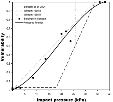
The calculated impact pressure vulnerability function was compared to two functions used in snow avalanche risk as-sessment (Fig. 12). Similar behaviour of the function can be noticed in comparison with the linear function of Barbolini et al. (2004) which was developed from avalanche data for West Tyrol, Austria. Wilhelm (1998) proposed two differ-ent relationships for vulnerabilities higher than 0.5: the for-mer (i) continues its linear trend and reaches vulnerability 1.0 at 34 kPa; the latter (ii) indicates that structures are consid-ered beyond repair in cases of impact pressures higher than 25 kPa. These functions of Wilhelm (1998) were calculated
B. Quan Luna et al.: The application of numerical debris flow modelling 2057 943
944 945
946 947 948
Figure 7
Figure 8
28
Fig. 8. Proposed vulnerability function for accumulation heights
obtained from the modelling.
949 950 951 952
953 954 955
Figure 9
Figure 10
Fig. 9. Proposed vulnerability function for modelled impact
pres-sures.
from data about reinforced structures impacted by avalanches in Switzerland. Compared to our equation, results using the Wilhelm (1998) functions vary a lot in lower vulnerabili-ties (up to 0.6). At vulnerability of 0.9 (33 kPa), our func-tion converges with the funcfunc-tion of Wilhelm (a) and reaches V=1.0 at 37.49 kPa. This is also different from Barbolini et al. (2004), who put vulnerability of 1.0 at impact pressure of 34 kPa (similar as Wilhelm, 1998).
950 951 952
953 954 955
Figure 9
Figure 10
29
Fig. 10. Proposed vulnerability function for accumulation heights
obtained from the modelling.
956 957
958 959
960 Figure 11
30
Fig. 11. Comparison of the proposed vulnerability functions
pro-posed by Akbas et al. (2009), Fuchs et al. (2007) and the vulnera-bility curve calculated from the Selvetta debris flow event in 2008.
The use of numerical modelling for the simulation of the dynamics of debris flows in the generation of vulnerability curves can present an advantage in terms that the intensity outputs (e.g. flow height and pressures) are straight forward and can be spatially displayed. The results can be over-laid with the elements at risk and detailed physical informa-tion can be obtained in a specific area. The approach pre-sented here can be assumed as an approximation of a building
2058 B. Quan Luna et al.: The application of numerical debris flow modelling
961
962 963 964 965 966 967 968 969 970 971
Figure 12
31
Fig. 12. Comparison of the proposed vulnerability functions
pro-posed by Barbollini et al. (2004), Wilhelm (1998), and the vulnera-bility curve calculated from the Selvetta debris flow event 2008.
resistance to endure a debris flow, which is information that is difficult to obtain directly on the field. Another important advantage in the employment of run-out models is that the intensity factors of the hazard can be analyzed in conjunc-tion with the physical vulnerability of the elements at risk, making it easier to quantify the suffered consequences. The aim to present different types of vulnerability curves in this analysis is to help the decision makers decide which type of intensity description best fits their needs and affected area. It can be argued that impact pressure vulnerability function can be used to measure the structure resistance itself, whereas using a flow height vulnerability function can also take into account the contents inside the structure.
The presented vulnerability functions do not conflict with the damage state probabilities functions that plot probabili-ties of the different damage states of a structure (e.g. slight damage, moderate damage, complete collapse). Whereas in the damage stage functions the proposed stages ranges are determined qualitatively in a subjective manner and the prob-ability of complete collapse can be smaller than 1, in the proposed vulnerability curves the degree of damage is deter-mined directly by the intensity of the event and a complete collapse takes a value of 1. For this reason, the values deter-mined by the vulnerability functions can be used directly in a quantitative risk assessment.
However, shortcomings in our analysis still exist and fur-ther research needs to be done regarding them. One of the major shortcomings is the insufficient data points regarding the affected elements at risk and the variation in values due to the differences in building quality, state, and structural char-acteristics. This should also be complimented by collecting
more data of damaged buildings affected by debris flows, or-ganizing them according to the type and use. This kind of de-scription plays a very important role for the analysis, as in the case where damage to buildings contents will be higher than to the building structure itself (i.e. shops and warehouses). Hence, a better estimation of the reported damage should be assessed based on structural and non-structural damage. A complete database with detailed information about building type, building use, building characteristics, building quality and state, and the amount of recorded damage (physical and economic), should lead to a better estimation of debris flow vulnerability curves.
There is also a high degree of uncertainty regarding the use of the model to simulate the different processes that played a key role in the evolution of the Selvetta debris flow event. Assumptions and empirical laws were used based on the need of inputs that FLO-2D model requires and the behaviour of the process (e.g. addition of sediment in the discharge hydro-graph to model the entrained material and peak discharge). Uncertainty regarding each modelled process has to be quan-tified in the future to reduce uncertainty. Although dynamic debris flow run-out models has been used with regularity in the past to reconstruct past events by calibration of the input parameters, there are still some limitations in the physical description of the parameters defining the applied rheology (quadratic).
Nevertheless, the presented approach attempts to propose a quantitative method to estimate the vulnerability of an ex-posed element to a debris flow that can be independent on the temporal occurrence of the hazard event.
Acknowledgements. This work has been supported by the Marie Curie Research and Training Network “Mountain Risks” funded by the European Commission (2007–2010, Contract MCRTN-35098). The authors would like to thank the reviewers for their comments, which improved the quality of the paper
Edited by: P. Reichenbach
Reviewed by: B. Pradhan and P. Gehl
References
Aleotti, P., Ceriani, M., Fossati, D., Polloni, G., and Pozza, F.: I fenomeni franosi connesi alle precipitazioni del Novembre 2002 in Valtellina (Soil slips and debris flows triggered by the novem-ber 2002 storms in Valtellina, Italian Central Alps), International Symposium Interpraevent 2004, Riva/Trient, Italy, 11–20, 2004. Barbolini, M., Cappabianca, F., and Sailer, R.: Empirical estimate of vulnerability relations for use in snow avalanche risk assess-ment, in: Risk analysis IV, edited by: Brebbia, C., WIT Press, Southampton, 533–542, 2004.
Bell, R. and Glade, T.: Quantitative risk analysis for landslides – Examples from B´ıldudalur, NW-Iceland, Nat. Hazards Earth Syst. Sci., 4, 117–131, doi:10.5194/nhess-4-117-2004, 2004. Bertrand, D., Naaim, M., and Brun, M.: Physical vulnerability of
reinforced concrete buildings impacted by snow avalanches, Nat. Hazards Earth Syst. Sci., 10, 1531–1545, doi:10.5194/nhess-10-1531-2010, 2010.
Calvo, B. and Savi, F.: A real-world application of Monte Carlo pro-cedure for debris flow risk assessment, Comput. Geosci., 35(5), 967–977, 2008.
Cancelli, A. and Nova, R.: Landslides in soil debris cover triggered by rainstorms in Valtellina (Central Alps – Italy), in: Proceedings of 4th International Conference and Field Workshop on Land-slides, The Japan Geological Society, Tokyo, 267–272, 1985. Cappabianca, F., Barbolini, M., and Natale, L.: Snow avalanche
risk assessment and mapping: A new method based on a com-bination of statistical analysis, avalanche dynamics simulation and empirically-based vulnerability relations integrated in a GIS platform, Cold Reg. Sci. Technol., 54(3), 193–205, 2008. Castellanos Abella, E. A.: Local landslide risk assessment, in:
Multi-scale landslide risk assessment in Cuba, edited by: Castel-lanos Abella, E.A., Utrecht, Utrecht University, ITC Disserta-tion, 154, 193–226, 2008.
Chen, H. and Lee, C. F.: Numerical simulation of debris flows, Can. Geotech. J., 37, 146–160, 2000
Chen, H., Crosta, G. B., and Lee, C. F.: Erosional effects on runout of fast landslides, debris flows and avalanches: A numerical in-vestigation, Geotechnique, 56(5), 305–322, 2006.
Chen, N. S., Yue, Z. Q., Cui, P., and Li, Z. L.: A rational method for estimating maximum discharge of a landslide-induced debris flow: A case study from southwestern China, Geomorphology, 84(1–2), 44–58, 2007.
Crosta, G., Marchetti, M., Guzzetti, F., and Reichenbach, P.: Morphological classification of debris-flow processes in South-Central Alps (Italy), Proceedings of the 6th International IAEG Congress, Amsterdam, 1565–1572, 1990.
Crosta, G. B., Dal Negro, P., and Frattini, P.: Soil slips and debris flows on terraced slopes, Nat. Hazards Earth Syst. Sci., 3, 31–42, doi:10.5194/nhess-3-31-2003, 2003.
Crosta, G. B., Fratinni, P., Fugazza, F., Caluzzi, L., and Chen, J.: Cost-benefit analysis for debris avalanche risk management, in: Landslide Risk Management, edited by: Hungr, O., Fell, R., Couture, R., and Eberhardt, E., Taylor & Francis, London, 533– 541, 2005.
DEI: Prezzi Tipologie Edilizie 2006, DEI Tipografia del Genio Civilie, CD-ROM, 2006.
Douglas, J.: Physical vulnerability modelling in natural hazard risk assessment, Nat. Hazards Earth Syst. Sci., 7, 283–288, doi:10.5194/nhess-7-283-2007, 2007.
Duzgun, H. S. B. and Lacasse, S.: Vulnerability and acceptable risk in integrated risk assessment framework, in: Landslide risk man-agement, edited by: Hungr, O., Fell, R., Couture, R., and Eber-hardt, E., Balkema, Rotterdam, 505–515, 2005.
Fell, R. and Hartford, D.: Landslide risk management, in: Landslide risk assessment, edited by: Cruden, D. and Fell, R., Balkema, Rotterdam, 51–109, 1997.
Fell, R., Ho, K. K. S., Lacasse, S., and Leroi, E.: A framework for landslide risk assessment and management, in: Landslide Risk Management, edited by: Hungr, O., Fell, R., Couture, R., and
Eberhardt, E., Taylor & Francis, London, 533–541, 2005. FLO-2D: Reference manual, 2009, available at: http://www.flo-2d.
com/wp-content/uploads/FLO-2D-Reference-Manual-2009. pdf, last access: 2010.
Fuchs, S., Heiss, K., and H¨ubl, J.: Towards an empirical vul-nerability function for use in debris flow risk assessment, Nat. Hazards Earth Syst. Sci., 7, 495–506, doi:10.5194/nhess-7-495-2007, 2007.
Galli, M. and Guzzetti, F.: Landslide Vulnerability Criteria: A Case Study from Umbria, Central Italy, Environ. Manage., 40(4), 649– 665, 2007.
Gamma, P.: DF-Walk: Ein Murgang-Simulationsprogramm zur Gefahrenzonierung (Geographica Bernensia, G66), University of Bern, 2000 (in German).
Glade, T.: Vulnerability assessment in landslide risk analysis, Die Erde, 134, 123–146, 2003.
Haugen, E. D. and Kaynia, A. M.: Vulnerability of structures im-pacted by debris flow, in: Landslides and Engineered Slopes, edited by: Chen, Z., Zhang, J.-M., Ho, K., Wu, F.-Q., and Li, Z.-K., Taylor & Francis, London, 381–387, 2008.
HAZUS-MH: HAZUS – FEMAs Methodology for Estimating Po-tential Losses from Disasters, available at: http://www.fema.gov/ plan/prevent/hazus/index.shtm, 2010.
Heinimann, H. R.: Risikoanalyse bei gravitativen Naturgefahren, Umwelt-Materialien, 107/1, 115 pp., 1999.
Hungr, O.: A model for the runout analysis of rapid flow slides, de-bris flows and avalanches, Can. Geotech. J., 32, 610–623, 1995. Jakob, M. and Weatherly, H.: Debris flow hazard and risk
assess-ment, Jones Creek, Washington, in: Landslide Risk Manage-ment, edited by: Hungr, O., Fell, R., Couture, R., and Eberhardt, E., Taylor & Francis, London, 533–541, 2005.
Kaynia, A. M., Papathoma-K¨ohle, M., Neuh¨auser, B., Ratzinger, K., Wenzel, H., and Medina-Cetina, Z.: Probabilistic assessment of vulnerability to landslide: Application to the village of Licht-enstein, Baden-W¨urttemberg, Germany, Eng. Geol., 101(1–2), 33–48, 2008.
Kwan, J. S. H. and Sun, H. W.: An improved landslide mobility model, Can. Geotech. J., 43, 531–539, 2006.
Leone, F., Ast´e, J. P., and Leroi, E.: Vulnerability assessment of elements exposed to massmovements: working toward a better risk perception, in: Landslides- Glissements de Terrain, edited by: Senneset, K., Balkema, Rotterdam, 263–270, 1996. Li, Z., Nadim, F., Huang, H., Uzielli, M., and Lacasse, S.:
Quanti-tative vulnerability estimation for scenario-based landslide haz-ards, Landslides, 7(2), 125–134, 2010.
Liu, X. and Lei, J.: A method for assessing regional debris flow risk: an application in Zhaotong of Yunnan province (SW China), Geomorphology, 52(3–4),181–191, 2003.
Luino, F.: Sequence of instability processes triggered by heavy rain-fall in the northern Italy, Geomorphology, 66(1–4), 13–39, 2005. Mavrouli, O. and Corominas, J.: Vulnerability of simple reinforced concrete buildings to damage by rockfalls, Landslides, 7(2), 169–180, 2010.
McClung, D. M.: Superelevation of flowing avalanches around curved channel bends, J. Geophys. Res., 106(B8), 16489–16498, 2001.
2060 B. Quan Luna et al.: The application of numerical debris flow modelling Muir, I., Ho, K. S. S., Sun, H. W., Hui, T. H. H., and Koo, Y. C.:
Quantitative risk assessment as applied to natural terrain land-slide hazard management in a mid-levels catchment, Hong Kong, in: “Geohazards”, edited by: Nadim, F., P¨ottler, R., Einstein, H., Klapperich, H., and Kramer, S., ECI Symposium Series, P07, 8 pp., 2006.
Nadim, F. and Kjekstad, O.: Assessment of global high-risk land-slide disaster hotspots, in: Disaster Risk Reduction, edited by: Sassa, K. and Canuti, P., Springer-Verlag, Berlin, 213–222, 2009. O’Brien, J. S. and Julien, P. Y.: Laboratory analysis of mudflow
properties, J. Hydraul. Eng., 114(8), 877–887, 1988.
O’Brien, J. S., Julien, P. Y., and Fullerton, W. T.: Two-dimensional water flood and mudflow simulation, J. Hydraul. Eng., 119(2), 244–261, 1993.
Pascale, S., Sdao, F., and Sole, A.: A model for assessing the systemic vulnerability in landslide prone areas, Nat. Hazards Earth Syst. Sci., 10, 1575–1590, doi:10.5194/nhess-10-1575-2010, 2010.
Prochaska, A., Santi, P., Higgins, J., and Cannon, S.: A study of methods to estimate debris flow velocity, Landslides, 5(4), 431– 444, 2008.
Remondo, J., Bonachea, J., and Cendrero, A.: Quantitative land-slide risk assessment and mapping on the basis of recent occur-rences, Geomorphology, 94(3–4), 496–507, 2008.
Rickenmann, D.: Debris Flows 1987 in Switzerland: Modelling and Sediment Transport (IAHS Publication No. 194, 371–378), In-ternational Association of Hydrological Sciences, Chrirstchurch, New Zealand, 1990.
Rickenmann, D.: Empirical Relationships for Debris Flows, Nat. Hazards, 19(1), 47–77, 1999.
Uzielli, M., Nadim, F., Lacasse, S., and Kaynia, A. M.: A concep-tual framework for quantitative estimation of physical vulnera-bility to landslides, Eng. Geol., 102(3–4), 251–256, 2008. van Asch, T. W. J., Malet, J.-P., van Beek, L. P. H., and Amitrano,
D.: Techniques, issues and advances in numerical modelling of landslide hazard, B. Soc. G´eol. Fr., 178(2), 65–88, 2007. van Westen, C. J., van Asch, T. W. J., and Soeters, R.: Landslide
hazard and risk zonation – why is it still so difficult?, B. Eng. Geol. Environ., 65, 167–184, 2006.
Whipple, K. X.: Predicting debris-flow runout and deposition on fans: the importance of the flow hydrograph, in: Erosion, Debris-Flows and Environment in Mountain Regions: Proceedings of the Chengdu Symposium, edited by: Walling, D., Davies, T., and Hasholt, B., International Association of Hydrological Sciences, 209, 337–345, 1992.
Wilhelm, C.: Quantitative risk analysis for evaluation of avalanche protection projects, in: Proceedings of the 25 Years of Snow Avalanche Research, Oslo, Norway, 288–293, 1998.
Zˆezere, J. L., Garcia, R. A. C., Oliveira, S. C., and Reis, E.: Proba-bilistic landslide risk analysis considering direct costs in the area north of Lisbon (Portugal), Geomorphology, 94(3–4), 467–495, 2008.