Clim. Past, 9, 1481–1493, 2013 www.clim-past.net/9/1481/2013/ doi:10.5194/cp-9-1481-2013
© Author(s) 2013. CC Attribution 3.0 License.
EGU Journal Logos (RGB)
Advances in
Geosciences
Open Access
Natural Hazards
and Earth System
Sciences
Open Access
Annales
Geophysicae
Open Access
Nonlinear Processes
in Geophysics
Open Access
Atmospheric
Chemistry
and Physics
Open Access
Atmospheric
Chemistry
and Physics
Open Access
Discussions
Atmospheric
Measurement
Techniques
Open Access
Atmospheric
Measurement
Techniques
Open Access
Discussions
Biogeosciences
Open Access Open Access
Biogeosciences
Discussions
Climate
of the Past
Open Access Open Access
Climate
of the Past
Discussions
Earth System
Dynamics
Open Access Open Access
Earth System
Dynamics
Discussions
Geoscientific
Instrumentation
Methods and
Data Systems
Open Access
Geoscientific
Instrumentation
Methods and
Data Systems
Open Access
Discussions
Geoscientific
Model Development
Open Access Open Access
Geoscientific
Model Development
Discussions
Hydrology and
Earth System
Sciences
Open Access
Hydrology and
Earth System
Sciences
Open Access
Discussions
Ocean Science
Open Access Open Access
Ocean Science
Discussions
Solid Earth
Open Access Open Access
Solid Earth
Discussions
The Cryosphere
Open Access Open Access
The Cryosphere
Discussions
Natural Hazards
and Earth System
Sciences
Open Access
Discussions
Bayesian parameter estimation and interpretation
for an intermediate model of tree-ring width
S. E. Tolwinski-Ward1, K. J. Anchukaitis2, and M. N. Evans3
1Institute for Mathematics Applied to Geosciences, National Center for Atmospheric Research, Boulder, CO, USA 2Woods Hole Oceanographic Institution, Woods Hole, MA, USA
3Department of Geology and Earth System Science Interdisciplinary Center, University of Maryland, College Park, MD, USA Correspondence to: S. E. Tolwinski-Ward ([email protected])
Received: 21 December 2012 – Published in Clim. Past Discuss.: 25 January 2013 Revised: 31 May 2013 – Accepted: 4 June 2013 – Published: 15 July 2013
Abstract. We present a Bayesian model for estimating the
parameters of the VS-Lite forward model of tree-ring width for a particular chronology and its local climatology. The scheme also provides information about the uncertainty of the parameter estimates, as well as the model error in rep-resenting the observed proxy time series. By inferring VS-Lite’s parameters independently for synthetically generated ring-width series at several hundred sites across the United States, we show that the algorithm is skillful. We also infer optimal parameter values for modeling observed ring-width data at the same network of sites. The estimated parameter values covary in physical space, and their locations in mul-tidimensional parameter space provide insight into the dom-inant climatic controls on modeled tree-ring growth at each site as well as the stability of those controls. The estimation procedure is useful for forward and inverse modeling studies using VS-Lite to quantify the full range of model uncertainty stemming from its parameterization.
1 Introduction
Forward models of the physical or biological processes by which climate variability is imprinted on natural archives provide important tools for understanding such “proxies” as recorders of climate (Evans et al., 2013). The VS-Lite model (Tolwinski-Ward et al., 2011) provides one such forward model for the climate controls on tree-ring width chronolo-gies. Under this model, just four parameters determine a sim-ulated chronology’s response to local mean monthly air tem-perature and monthly model-simulated soil moisture. These
parameters connect the local climatology to the modeled con-trols on growth and the climatic signal contained in the sim-ulated chronology. Thus, in order to use VS-Lite to study the relationship between climate and proxies in the real world, an objective method for choosing the model parameters for any particular site or region is necessary.
limited ability of direct observations to constrain the model parameters, it is necessary to estimate VS-Lite’s parameters numerically using monthly climate inputs, observed ring-width series, and partial knowledge of the model error struc-ture. At sites where VS-Lite is believed to provide a reason-able intermediate complexity proxy system model for tree-ring width variations, such an estimation procedure can also be used to estimate the parameters of the error model aris-ing from the model’s incomplete representation of the proxy system.
Three general approaches to objective numerical param-eter estimation of forward models of tree-ring growth have been explored in the literature. The first is presented by iter-ative local schemes that optimize the fit of simulated model quantities to their observed counterparts under changing pa-rameter combinations. In the iterative scheme of Fritts et al. (1999), for example, one model parameter is changed at a time in a search over a continuous region of parameter of space for the set of parameters producing optimal model fit. Modern computing power makes such schemes possible to run at many locations, but the approach does not account for potential interactions between parameters. The scheme may also locate a local optimum in parameter space but miss in-formation, including other optima, provided by a more global search. A second class of approaches attempts to avoid this last pitfall by running growth models at a preselected, dis-cretized set of parameter combinations believed to cover the entire physically plausible regions of parameter space, and the single combination that produces the best match of mod-eled outputs to its observed counterparts is deemed optimal (e.g., Misson et al., 2004; Misson, 2004; Tolwinski-Ward et al., 2011). This parameterization method is only practi-cal where the number of parameters to be constrained by the available data is relatively small. Both local and global previ-ous parameterization schemes have the shortcoming that they provide only point estimates of optimal parameters, and their results do not include any information about model sensitiv-ity to the parameter choices. In addition, while the ranges of parameters included in the search space are generally cho-sen through consideration of physically plausible bounds on their values, the search algorithms lack any more sophisti-cated use of science-based understanding of where the most likely parameter values lie. Bayesian modeling and inference represents a third approach in which conditional probability distributions of the unknown parameters are inferred given the information in model input climate data and observed se-ries of tree-ring width data. Because the product of such an analysis is a probability distribution, the Bayesian approach also has the advantage of automatically providing uncertainty and sensitivity estimates along with parameter estimates. The approach also automatically safeguards against over-tuning when the calibration data series are short and/or noisy. Such an approach was explored by Gaucherel et al. (2008) to in-fer the parameters of a complex, biology-resolving model of tree-ring growth. Although not a forward model of tree-ring
width given climate, work by Boreux et al. (2009) also em-ployed a Bayesian approach to estimate a latent regional tree-ring width signal and the parameters of an accompanying hierarchical model to interpret several neighboring tree-ring width chronologies.
Here we present and test a Bayesian statistical model to infer parameter estimates for VS-Lite for simulating a particular chronology from co-located climatic inputs. Our scheme is efficient enough to run in a matter of minutes in a modern laptop computing environment, and returns probabilistic posteriors that can be analyzed to infer uncer-tainty and sensitivity information as described above. In ad-dition, the scheme takes particular advantage of the capa-bility of the Bayesian framework to assimilate expert sci-entific prior knowledge into the inference. Version 2.3 code for the scheme is freely available with the VS-Lite v2.3 model at the National Oceanic and Atmospheric Admin-istration (NOAA) Paleoclimatology software library (http: //www.ncdc.noaa.gov/paleo/softlib/softlib.html). We test the skill of the parameterization approach in several hundred in-dependent idealized experiments using synthetically gener-ated tree-ring width data. As an application of the method to observed ring-width chronologies, we also independently es-timate parameters for several hundred observed chronologies across the continental United States and present a graphical method for interpreting the fitted model parameters in terms of climatic controls on tree-ring growth at each site.
2 Model, data, and methods
While climate is a spatiotemporal phenomenon, and net-works of tree-ring width can be used to make inferences about the past space–time variations in climatic fields, trees only experience and respond to their local environments. This is reflected in the structure of VS-Lite, which models tree-ring width variations as a function of local climate. Here we take the view that the model provides a first-order repre-sentation of the general mechanisms by which climatic vari-ability is imprinted on all climatically sensitive trees. Within this framework, VS-Lite’s growth response parameters and the parameters of an accompanying error model adjust the re-sponse of VS-Lite to fit better the observed growth rere-sponses that vary from site to site depending on species, specific lo-cal environmental conditions, and the varying sensitivity of the signal in individual tree-ring width series that compose a given chronology.
2.1 Summary of VS-Lite and parameters
growth (Vaganov et al., 2006, 2011). At its core, VS-Lite is a parsimonious representation of the Principle of Limit-ing Factors with respect to local monthly temperature and soil moisture, and with growth modulated by local insolation. In its current version (version 2.2), insolation is determined from site latitude, and soil moisture is determined from local monthly temperature and precipitation via a simple bucket model (Huang et al., 1996). Non-dimensional scaled growth responsesgT(m, y)andgM(m, y)to monthly time-step
tem-perature and soil moisture content, respectively, are key to determining the extent of simulated growth in each modeled monthmand yeary. These responses have the piecewise lin-ear forms
gT(m, y)=
0 T (m, y)≤T1;
T (m,y)−T1
T2−T1 T1≤T (m, y)≤T2;
1 T2≤T (m, y)
(1)
and
gM(m, y)=
0 M(m, y)≤M1;
M(m,y)−M1 M2−M1 M1
≤M(m, y)≤M2;
1 M2≤M(m, y)
(2)
The parameters T1 and M1 thus represent thresholds
in temperature and soil moisture content below which growth cannot occur, while T2 and M2 are thresholds
above which growth is insensitive to climatic variability. The overall monthly growth rate is given by g(m, y)=
min{gT(m, y), gM(m, y)}, to mimic the Principle of
Limit-ing Factors (Fritts, 2001) that the more limitLimit-ing environmen-tal variable controls growth. The simulated annual-resolution ring-width series result from taking an inner product of these overall growth rates with estimates of mean relative monthly insolation derived from trigonometric functions of latitude. Thus, the climatic variable that tends to produce lesser val-ues in its growth response function controls the modeled cli-mate signal contained in the simulated proxy series. The re-lationship of the parameter valuesT1, T2, M1, and M2 to
the model’s climate inputs is therefore critical in determin-ing which variable gets “recorded” by the synthetic trees.
We denote byWˆ VSL, the deterministic VS-Lite estimate
of a tree-ring width series given fixed temperature and pre-cipitation inputs and fixed VS-Lite growth response parame-tersθVSL=(T1, T2, M1, M2)0. Formally, we model the
zero-mean, unit-variance time series of ring-width data W at a location of interest by a scaling of the VS-Lite output plus stochastic noise to account for non-climatic noise in the data and for the effects on the time series of processes that VS-Lite does not resolve:
W= q
1−σW2Wˆ VSL+e (3)
with σW2 =Var(et) .
We allow for the possibility that the time series of er-rors e may follow either a white noise model, so thatet∼
N (0, σW2), or else an AR(1) model,et∼N (φ1et−1, τ2), with
the conditions for stationarity for the noise process imposing
σW2 = τ2 1−φ2
1
in the latter case (Shumway and Stoffer, 2006). Since both the time series of data and of VS-Lite output are standardized to have zero mean and unit variance, the coef-ficient
q
1−σW2 on the estimate from VS-Lite gives the pro-portion of the observed data’s standard deviation that can be explained by VS-Lite as “signal”, and so the signal-to-noise ratio is SNR=
r 1−σW2
σ2
W
. We write the parameters of the er-ror model asθe=σW2 for white noise andθe=(φ1, τ2)T for
AR(1) errors. We treat these as additional model parameters to be estimated at any given site, whose values provide in-formation about the degree to which VS-Lite can be used to explain the observed variations in the data.
2.2 Approach to model parameter estimation
We follow a Bayesian approach to estimating the model pa-rameters at a particular location. Letθdenote the vector of model parameters we would like to estimate, and W(T,P)
the vector of observed ring-width data, which depends on vectors of monthly temperature and precipitation data cov-ering the same interval in time as the ring width data. The Bayesian paradigm allows inference on the posterior distri-butionπ(θ|W(T,P))of the parameters given the climate and ring width data in terms of the likelihoodf (W(T,P)|θ)of the ring-width data given the climate and the parameters, as well as a prior distributionπ(θ)on the parameters via Bayes’ law:
π(θ|W(T,P))∝f (W(T,P)|θ)π(θ). (4) Given the likelihood and prior parameter models, Markov chain Monte Carlo techniques produce an ensemble of draws from the posterior distribution (Gilks et al., 1996), from which estimates of the parameters and their associated un-certainties can be made.
In the present setting, the parametersθ consist of the set
θVSL=(T1, T2, M1, M2)T used to compute the
determinis-tic response of VS-Lite to input climate data, and the setθe
that describe the VS-Lite model error structure, so thatθ=
(T1, T2, M1, M2,θe)T. Given the data-level model in Eq. (3),
the likelihood in Eq. (4) may be thus be written as
f (W(T,P)|θ)∝ 1 |6e|1/2
exp (5)
−1
2(W−
q
1−σW2WˆVSL)T6e−1(W− q
1−σW2Wˆ VSL)
.
Note that the dependence onθVSLis implicit in the estimate ˆ
WVSL, which is computed for a particular set of growth
re-sponse parameters. The dependence on the error model pa-rametersθeis through the covariance matrix6eand the noise
whether a white noise or AR(1) noise model is appropriate at a particular site; these details are discussed in the supplemen-tary material. Note that in its current version, VS-Lite also requires several parameters of the Leaky Bucket model of soil moisture (Huang et al., 1996). We do not estimate those here, as the soil moisture model may be viewed as an ancil-lary component of VS-Lite that may be replaced by a more sophisticated hydrological model or direct measurements of soil moisture. In effect, our current approach transfers the uncertainty associated with these parameters to uncertainty in the soil moisture response parametersM1andM2.
In modeling the prior distribution of the VS-Lite growth response parameters, we first make the assumption that each parameter is independent of the others. This assumption al-lows us to model their joint prior distribution as the prod-uct of individual prior models for each. We put relatively broad but informative priors on the growth response param-eters, with shapes and supports consistent with current sci-entific understanding of tree growth responses to tempera-ture and moistempera-ture. While the original full VS model was built around conifer physiology, VS-Lite is a generalized im-plementation of the principle of limiting factors and piece-wise growth functions, and should be a valid representa-tion of growth in both gymnosperms and angiosperms. Al-though it is conceivable that different priors might be con-structed for different tree species, it is difficult to disentan-gle the influence of species on growth response from the influences of specific site characteristics, non-climatic influ-ences, and random effects, and no comprehensive identifi-cation of the differences in growth response exists for the dozens of species used for dendrochronology. We thus con-struct species-independent priors using general information about growth across all climate-sensitive trees.
Of the four growth response parameters, the literature pro-vides the most information aboutT1, the threshold
temper-ature for growth to begin. The physiological experiments of K¨orner and Hoch (2007) at a montane site in Switzerland in-dicated that mean seasonal soil temperatures below 6–7◦C would not permit growth. An assessment of root and air tem-peratures at a few dozen tree-line sites by K¨orner and Paulsen (2004) gave a value of 6.7±0.8◦C for this growth thresh-old, and histological measurements and analyses of Rossi et al. (2007) and Deslauriers et al. (2008) for conifers in the Alps gave a range of 5.8–8.5◦C. Hoch and K¨orner (2009) found that two montane conifer species maintained cambial activity even when grown at 6◦C. K¨orner (2012) inferred a
global mean tree-line isotherm near 6◦C and cessation of
growth at 5◦C (K¨orner, 2008); 0◦C is the theoretical limit
below which plant tissue formation cannot occur (K¨orner, 2012). We thus chose to model the temperature threshold for growth byT1∼β(9,5,0,9), a four-parameter beta
distribu-tion with shape parametersα=9 andβ=5 supported on the interval[0,9]. This choice puts the mode of the probabil-ity densprobabil-ity function at 6◦C, assigns zero probability below freezing (0◦C) or above 9◦C, and places 90 % of the total
probability in the interval (3.8◦C, 7.5◦C) (see blue curve in
Fig. 1a and e).
The biologically based information available aboutT2, the
threshold above which growth is no longer sensitive to tem-perature variations, is more uncertain. Vaganov et al. (2006) give a default value of 18◦C for the full Vaganov–Shashkin model based on a few intensive case studies at a limited num-ber of Russian tree-ring sites, but use a value of 15◦C in an example model run, demonstrating the range of uncertainty associated with this parameter. The analogous parameter in the TreeRing2000 model has a default value of 23◦C (Fritts et al., 1999). Data shown by Williams et al. (2011) suggest a broad plateau where ring width in Alaskan Picea glauca ceased increasing with June and July mean temperatures be-tween approximately 10 and 13◦C, depending on site hy-drology. On the other hand, Garfinkel and Brubaker (1980) showed no change in the regression of ring width on temper-ature in the same species even at tempertemper-atures approaching 15◦C. Carrer et al. (1998) inferred a lower optimal summer temperature threshold of 13◦C for Picea abies and 16◦C for
Larix decidua. Although this information sheds some light
on the threshold for sensitivity to temperature, the majority of these studies are based on empirical data at monthly to seasonal timescales, as opposed to direct studies of cambial activity in response to temperature. To reflect the uncertainty inherent in the wide range of these estimates, as well as un-certainty in their direct applicability as parameter estimates in VS-Lite, we model the prior byT2∼β(3.5,3.5,10,24).
This choice limits probability mass to the interval (10◦C, 24◦C), and distributes probability symmetrically about a mean of 17◦C with a standard deviation of 2.5◦C, and 90 %
of the total probability in the interval (12.9◦C, 21.1◦C) (blue
curve, Fig. 1b and f).
Very little biologically based information is available to constrain either moisture parameter. We use the default pa-rameters developed by Vaganov et al. (2006) to define broad priors onM1andM2. Default values for M1, interpretable
as soil wilting point, are 0.02 v / v (Vaganov et al., 2006) and 0.01 v / v (Fritts et al., 1999). The latter source also sets a moisture optimum at 0.109 v / v, so the value ofM1
should certainly fall well below this value. We set the prior mean at 0.035 with standard deviation of 0.02 v / v, with no probability mass outside of (0 v / v, 0.1 v / v), by letting
M1∼β(1.5,2.8,0,0.1), with the interval (0.006 v / v, 0.073
v / v) containing 90 % of the prior probability (blue curve, Fig. 1c and g). The default forM2is 0.8 of typical soil
satu-ration levels, and the Leaky Bucket model of soil moisture employed by VS-Lite never allows soil to be saturated to a value more than 0.75 v / v (Huang et al., 1996). We set
M2∼β(1.5,2.5,0.1,0.5). This gives the prior a mean of
0.25 v / v, a standard deviation of 0.1 v / v, nonzero probabil-ity on (0.1 v / v, 0.5 v / v), and 90 % of the prior probabilprobabil-ity mass in (0.125 v / v, 0.406 v / v) (blue curve, Fig. 1d and h).
In assigning priors to the parameters θe, we enforce
Prior (blue) and posterior (red) densities of VS−Lite parameters, Pseudoproxy Experiments
0 2 4 6 8 0
0.1 0.2 0.3 0.4
T1, SNR = 1
° C a)
10 15 20 0
0.1 0.2 0.3 0.4
T2, SNR = 1
° C b)
0 0.05 0.1 0
5 10 15 20
M1, SNR = 1
v/v
c)
0.1 0.2 0.3 0.4 0.5 0
5 10 15 20 25
M2, SNR = 1
v/v
d)
0 2 4 6 8 0
0.1 0.2 0.3 0.4
T1, SNR = 0.25
° C e)
10 15 20 0
0.05 0.1 0.15 0.2
T2, SNR = 0.25
° C f)
0 0.05 0.1 0
5 10 15 20
M1, SNR = 0.25
v/v
g)
0.1 0.2 0.3 0.4 0.5 0
1 2 3 4 5
M2, SNR = 0.25
v/v
h)
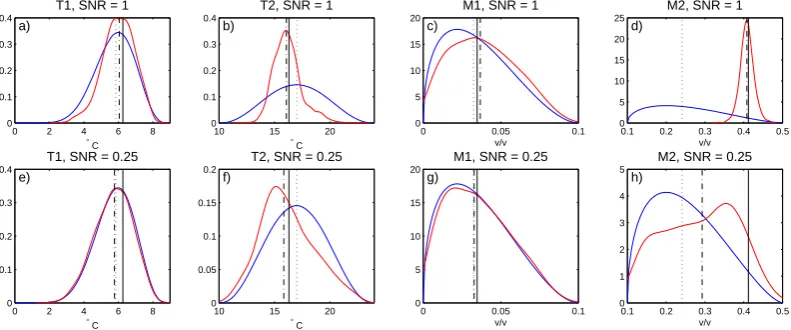
Fig. 1. (a–d)Prior (blue) and estimated posterior (red) densities for the parameters of VS-Lite at the Sipsey Wilderness site in Alabama, for
the pseudoproxy experiment with SNR = 1. Plot of posterior density given by a kernel smoothing of the frequency distribution of ensemble members. Solid black vertical lines give the target values of the growth response parameters, dotted black lines prior medians, and dash-dot black lines the posterior medians. (e–h) As in (a–d), but for PPE with SNR = 0.25.
magnitude of the process be no greater than the unit-variance observations, and require that the lag-1 autocorrelation be non-negative, but do not supply the priors with any other information. For the white-noise model, these criteria re-sult in a prior σW2 ∼U (0,1). For the AR(1) model, they imply a normalized indicator function on the set {φ1, τ2:
φ1∈(0,1), τ2< (1−φ12)}(see, e.g., Shumway and Stoffer,
2006). At each site the parameter estimation procedure is first run assuming white errors. The residuals of simulated ring-width index using the posterior median growth response parameters are then fit with a white noise error model and an AR(1) model. If the AR(1) model has a lesser value of Schwarz’s Bayesian criterion (Robert, 2007, Sect. 7.2.3), then the parameter calibration is re-run for that site under the assumption of AR(1) model errors.
The posterior distribution (Eq. 4) is sampled using a Metropolis–Hastings algorithm embedded within a Gibbs sampler, which is a standard Markov chain Monte Carlo (MCMC) approach (Chib and Greenberg, 1996). To check for convergence, we run three chains with 30 000 iterations each after a burn-in period of 300 iterations. In the rare case that the R-hat statistic (Gelman and Rubin, 1992) indicates the MCMC has not converged, we re-run the sampler with a greater number of iterations until the sampler has converged. The autocorrelation functions of the MCMC chains indicate that, at most sites, autocorrelation in the parameter sampling chains is no longer significant past a lag of 20. We conserva-tively subsample every 50th value of each of the 3 chains to ensure independence of samples, resulting in a collection of 1800 samples for each parameter value at each site.
The ensemble output may be used in several different ways. First, point estimates from the posterior ensemble,
such as the posterior median or the maximum likelihood pa-rameter set, may be used as calibrated papa-rameter values that optimize the fit between model-simulated ring width data and a target ring width series, given fixed input climate data. However, the posteriors contain additional information be-yond point estimates. Their spread indicates the uncertainty in the parameter estimates, as well as the degree to which the climate and target ring-width data inform the parameter values. Hence a measure of the model sensitivity to each pa-rameter may also be gleaned from the posterior spread. The Monte Carlo ensemble of parameter values may also be used to run modeling studies where accounting for the effect of parameter uncertainty is important for interpretation of the results.
2.3 Experimental design
Paleoclimate Reconstructions Network/Proxy Data webpage (http://www.ncdc.noaa.gov/paleo/pubs/pcn/pcn-proxy.html.
2.3.1 Pseudoproxy experiment (PPE)
To evaluate the skill of the Bayesian parameter estimates, we perform two so-called “pseudoproxy experiments” (PPEs) (Smerdon, 2012) using synthetically generated tree-ring width data. At each site, we first perform a preliminary run of the Bayesian scheme described above using the observed chronologies and PRISM-derived climate data for the inter-val 1895–1984. The sampling scheme is run to convergence with a white noise model at each site, but at sites where the residuals between VS-Lite estimates and the observed data display temporal autocorrelation, the sampling scheme is re-run with the AR(1) noise model. The posterior medians and the estimated noise models from this step parameterize re-gionally realistic tree growth responses to climate, and com-prise a set of known PPE parameter targets that we try to recover to test our methodology. We run the VS-Lite model over the same interval using this target parameter set and the PRISM climate estimates to produce 277 synthetic ring-width signals. We scale the simulated signal and add noise according to Eq. (3) such that the signal-to-noise ratio (SNR) is 1 in the first PPE, and is SNR = 0.25 in the second PPE. These values represent optimistic and pessimistic estimates of the SNRs of real-world proxies, respectively (Smerdon, 2012), and the resulting 277 time series constitute the syn-thetic data set we use to infer the known parameter values us-ing the Bayesian scheme. In this inference step of the PPEs, we condition on the known climate data and pseudoproxy ring-width data over the entire interval to estimate the growth response parameters and error model parameters. The form of the error model (white or AR(1)) at each site is also as-sumed known, rather than inferred. The PPEs are designed as a test of our parameter calibration scheme over a realistic range of tree responses to climate, but in an idealized model world where both the signal-formation and noise processes are perfectly known and represented except for the value of their parameters. The ability of the parameter inference pro-cedure to recover the known target parameters in the PPEs thus provides an upper bound on the skill for the procedure in real-world scenarios.
Comparing the growth parameter posterior distributions to the known targets allows us to quantify the skill of the esti-mation scheme. The numerics returnN=1800 draws from the posterior distribution, so we compute Monte Carlo esti-mates of the root-mean-square error and bias in the pseudo-proxy context using the “true” target parameter valuesθ:
RMSE≈ v u u t
1
N
N X n=1
(θˆn−θ )2; (6)
Bias≈ 1
N
N X n=1
(θˆn−θ ). (7)
The extent to which the prior and posterior distributions dif-fer indicates the degree to which the climate, ring-width data, and the VS-Lite model structure constrain the value of each parameter. To quantify this “Bayesian learning” at each site, we examine the ratio of posterior to prior variance. Parame-ters whose posteriors are well-constrained by the data will have much smaller posterior variance than prior variance, while parameters that are not well-constrained will have pos-teriors that resemble their priors, and hence variance ratios close to one. Finally, we compute the estimated signal-to-noise ratios by the posterior median of
r 1−σW2
σ2
W
, and compare to the known SNR used to construct the synthetic data across the 277 sites.
2.3.2 Observed proxy model calibration (OPMC)
We also calibrate the VS-Lite model parameters indepen-dently at each of the 277 network sites to perform an ob-served proxy model calibration (referred to hereafter by the acronym OPMC). The estimates of the growth response pa-rameters are conditioned on the PRISM-derived climate se-ries and observed ring-width index sese-ries for the 45 yr in-terval 1940–1984, and the parameters of the error model are estimated using the data in the complementary 45 yr in-terval 1895–1939. Split calibration/validation inin-tervals help prevent calibration of artificial skill when selecting parame-ters (Cook et al., 1999; Evans et al., 2002). We also perform the analysis with the growth parameter and error parameter calibration intervals reversed to gauge the dependence of the calibration on the choice of calibration interval.
months over the entire simulation in which the growth re-sponse to soil moisture (temperature) is strictly less than the growth response to temperature (soil moisture). If the mod-eled proportion is significantly more than the null hypothesis of half, then the site is classified asM-limited (T-limited). Sites for which the proportion cannot be statistically distin-guished from 0.5 are classified as mixed-control sites. We then examine the structure of the parameter point estimates in multi-dimensional parameter space for each class of sites. To evaluate the sensitivity of the parameter estimation scheme to the choice of prior distributions, the observed proxy model calibration described above is also performed with uniform prior distributions with the same supports as those for the literature-informed four-parameter beta priors described in Sect. 2.2. The uniform prior is a standard non-informative choice against which to check the sensitivity of posterior results to more complicated priors (see Gelman et al., 2003, Sect. 6.8). The posteriors derived under the four-parameter beta priors informed by the literature are compared with those derived using the uniform priors.
3 Results
For a single site, the parameter estimation procedure de-scribed here can be run on a MacBook Pro with 2.7 GHz processor in under 3.5 min for three chains of length 30 300 in series when the white noise model is used, and in close to 9 min when the AR(1) error model is used.
For the experiments performed here, trace plots of the MCMC chains and R2 statistics close to 1 both indicated that the samples had converged adequately (see Supplement Fig. 1 for trace plots at a representative site). The proce-dure returns 106 out of 277 sites with a white noise error model, and 171 sites with an AR(1) error model when run using the observed data. At two representative sites, one us-ing the white noise error model and one usus-ing the AR(1) error model, the reproducibility of the point estimates was checked by running the estimation procedure twice for the PPE with SNR = 1 and for the OPMC. In both cases, the dif-ference between estimates of the two temperature thresholds
T1 andT2 from two runs of the algorithm was less than a
tenth of 1◦C; moisture thresholds M1 andM2were
repro-duced to within 0.004 v / v (so the percentage change in the value of the point estimates of the growth parameters is less than 1 % except forM1, which is reproduced to within 6 %).
The ratio of posterior to prior variance was reproduced in all cases to within 0.05 (percent change of less than 7 % ex-cept for M1, to within 11 %), and the estimated
signal-to-noise ratios were within 0.02 of one another (reproduced to less than 0.2 %) for the two runs (further details are in the Supplementary Tables 1 and 2).
−0.6 −0.4 −0.2 0 0.2 0.4 0.6 0
0.1 0.2 0.3 0.4 0.5 0.6
RMSE/prior range
posterior/prior bias
T1
a) SNR = 1 SNR = 0.25
−0.6 −0.4 −0.2 0 0.2 0.4 0.6 0
0.1 0.2 0.3 0.4 0.5 0.6
RMSE/prior range
Bias/prior range
T2
b)
−0.6 −0.4 −0.2 0 0.2 0.4 0.6 0
0.1 0.2 0.3 0.4 0.5 0.6
RMSE/prior range
Bias/prior range
M1
c)
−0.6 −0.4 −0.2 0 0.2 0.4 0.6 0
0.1 0.2 0.3 0.4 0.5 0.6
RMSE/prior range
Bias/prior range
M2
d)
0.5 1 1.5 0
10 20 30 40 50 60 70
Posterior median SNR Experiment with pseudoproxy SNR = 1 e)
0 0.2 0.4 0.6 0.8 1 0
20 40 60 80 100
Posterior median SNR Experiment with pseudoproxy SNR = .25 f)
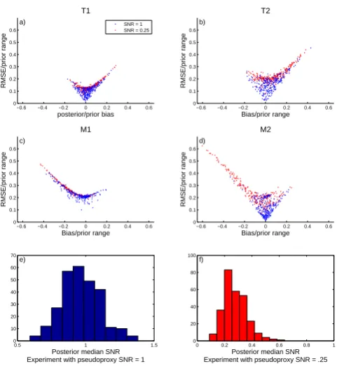
Fig. 2. (a–d) root-mean-squared error versus bias of parameter
esti-mates in the pseudoproxy experiment, with both statistics shown relative to the length of each prior’s support for the PPE with SNR = 0.25 (red) and SNR = 1 (blue). Note that the structure in the scatter plots is a result of the fact that by definition RMSE(X)= q
Var(X)+Bias2(X). (e) Histogram of median posterior estimated signal-to-noise ratio (SNR) across all 277 sites, for the pseudoproxy experiment where the true SNR = 1. (f) As in (e) but for the experi-ment with SNR = 0.25.
3.1 Pseudoproxy experiment (PPE) results
A plot of prior and smoothed posterior distributions of the four growth response parameters for one representative site in the network is shown in Fig. 1 for both PPEs. The varia-tion in learning between parameters is evident in this figure, as conditioning the data tends to inform values ofM2 and
T2 to a greater extent at this particular site than the lower
thresholdsT1andM1. Comparing the shape of the posteriors
between pseudoproxy experiments also shows that the data inform the estimation to a greater (lesser) degree when the data have higher (lower) signal-to-noise ratio. A set of such posterior distributions exists for every site in the experimen-tal network, and we compute statistics on these distributions to assess the skill of the parameter calibration method.
Both posterior bias and root-mean-squared error tend to be on the order of 20 % or less of the length of the prior interval for estimates of the parameters (Fig. 2a, b, d). The negative bias for the parameterM2 in the experiment with
120° W 110°
W 100° W 90° W 80° W 70
° W
30° N 40° N
50° N T1
0 0.5 1
120° W 110°
W 100° W 90° W 80° W 70
° W
30° N 40° N
50° N T2
0 0.5 1
120° W 110°
W 100° W 90° W 80° W 70
° W
30° N 40° N
50° N M1
0 0.5 1 0 0.5 1
Ratio of Posterior to Prior Variance, PPE(SNR=1)
120° W 110°
W 100° W 90° W 80° W 70
° W
30° N 40° N
50° N M2
Fig. 3. Ratio of posterior to prior variance for the four growth
re-sponse parameters as a measure of Bayesian learning in the pseu-doproxy experiment with SNR = 1. The color scale is calibrated so that sites with values of the ratio greater than/equal to one/less than one have blue/white/red coloration.
SNR experiment suggests that the bias is an artifact of the choice of prior distribution being centered at lower values than those that seem to fit the data best. Figure 2e and f show histograms of the posterior median values of the es-timated signal-to-noise ratios in both experiments across the 277 sites. The individual estimates of SNR vary from site to site because each posterior is conditioned on only a single realization of the noisy synthetic ring-width data. Across the independent posteriors at all sites, however, the distributions of the estimates are centered on the correct SNR values for the respective experiments.
The ratio of posterior to prior variance is shown in Fig. 3 for the PPE with unit SNR. In general, “Bayesian learning” tends to be high for the upper thresholdsT2andM2, as
ev-idenced by ratios less than one at most sites across the net-work. This result is indicative of high model sensitivity to the value of these parameters. By contrast, more sites have variance ratios close to one for the parameterT1, especially
in the southern United States and along the southeastern seaboard of the United States, and most sites across the net-work have variance ratios near one for the parameterM1.
Thus the marginal posteriors ofT1andM1at these sites are
similar in spread to the priors, indicating model insensitiv-ity to their values. The variance ratios are higher across all variables and sites for the PPE with lower signal-to-noise ra-tio (Supplement Fig. 2), which is consistent with the general expectation that noisier data cannot constrain the solution as well as less noisy data.
3.2 Observed proxy model calibration (OPMC) results
The point estimates of the VS-Lite parameters in the ob-served proxy model calibration experiments, given by the posterior medians, show some spatial structure (Fig. 4). Al-though the varying network density makes it difficult to dis-tinguish geographical patterns, parameters do tend to take on values close to those of their nearest neighbors. In particular, the estimated values ofT2tend to occupy the lower end of
120° W 110
° W 100° W 90° W 80° W 70
° W
30° N
40° N
50° N T1
0 2 4 6 8
120° W 110
° W 100° W 90° W 80° W 70
° W
30° N
40° N
50° N T2
10 15 20
120°
W 110° W 100° W 90° W 80° W 70
° W
30° N 40° N
50° N M1
0 0.02 0.04 0.06 0.08 0.1 0.1 0.2 0.3 0.4 0.5
Parameter point estimates inferred with observed data constraints
120°
W 110° W 100° W 90° W 80° W 70
° W
30° N 40° N
50° N M2
Fig. 4. Posterior medians of VS-Lite growth parameters. Note that
the color scale for each parameter ranges over the interval on which the prior is supported, and is calibrated so that white indicates the prior median.
120° W 110°
W 100° W 90° W 80° W 70
° W
30° N 40° N
50° N T1
0 0.2 0.4 0.6 0.8 1
120° W 110°
W 100° W 90° W 80° W 70
° W
30° N 40° N
50° N T2
0 0.2 0.4 0.6 0.8 1
120° W 110
° W 100° W 90° W 80° W 70
° W
30° N
40° N
50° N M1
0 0.2 0.4 0.6 0.8 1 0 0.2 0.4 0.6 0.8 1
Ratio of Posterior to Prior Variance, OPMC
120° W 110
° W 100° W 90° W 80° W 70
° W
30° N
40° N
50° N M2
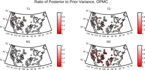
Fig. 5. Ratio of posterior to prior variance for the four growth
re-sponse parameters as a measure of Bayesian learning in the ob-served proxy experiment. The color scale is calibrated so that sites with smaller (larger) values of the ratio, indicating greater (lesser) Bayesian learning, have darker (lighter) coloration.
the prior support in the west of the United States, with more variation between sites east of the Continental Divide. Val-ues ofM1also tend to fall near the upper end of the prior for
arid and semi-arid sites in the west. Point estimates ofM2are
close to the upper end of the prior range at most sites across space, and preferred values ofT1tend to be close to the prior
median but show some variation for sites within close range of one another.
The spatial distribution of Bayesian learning, parameter-ized by the ratio of posterior to prior variance, is highest for the parameterM2away from the eastern seaboard and
north-ernmost Pacific Northwest sites (Fig. 5). This result indicates that simulations of the data are sensitive to this parameter at all but those sites. Sites with high and low Bayesian learning on the parameterT2are interspersed throughout the domain.
The parametersT1 and especially M1 appear to have very
little influence on the data, as conditioning on the data con-strains their posterior distributions little if at all.
0 0.2 0.4 0.6 0.8 1 1.2 1.4 1.6 1.8 2 0
0.5 1 1.5 2
Estimated SNR
Calibrated 1940−1984
Calibrated 1895−1939
120° W
110° W 100° W 90° W 80° W 70
° W
30° N 40° N
50° N Posterior Median SNR
0.3 0.4 0.5 0.6 0.7 0.8 0.9 1
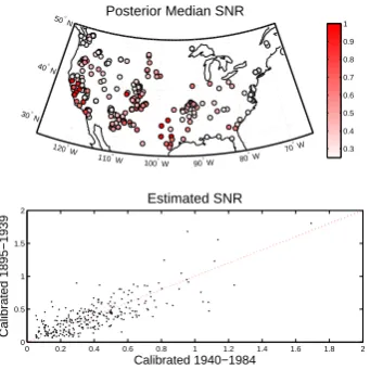
Fig. 6. Top: map of posterior median signal-to-noise ratio (SNR)
across sites in network, estimated by comparing simulated and ob-served data during 1895–1939. Bottom: comparison of posterior median SNR estimated during 1895–1939 and 1940–1984 for val-ues of growth response parameters estimated using data in the com-plementary intervals.
which VS-Lite can be used to explain the observed ring-width chronologies. The posterior median signal-to-noise ra-tios are similar when estimated during the first and second halves of the 90 yr interval (bottom panel), indicating robust-ness in the model performance to the choice of calibration interval, and the posterior median SNR estimated between 1940 and 1984 is within 1, 2, and 3 posterior standard devi-ations of the posterior median SNR estimated between 1895 and 1939 for 55, 87, and 95 % of sites respectively.
Calibration of the parameters improves the skill of the VS-Lite simulations in predicting the observed data. The correla-tion of the simulated ring width with observacorrela-tions in the com-plement of the interval used to estimate the growth response parameters increases uniformly across the sites (Fig. 7, left panel). At the Andrew Johnson Woods site in Ohio, for ex-ample, the correlation of calibrated (uncalibrated) simulated ring width with observations is typical of this metric of skill across chronologies simulated in this study, atρ=0.30 (ρ= −0.13) with the observed ring-width time series. In fact, cal-ibrating the parameters at this representative site is crucial in determining the simulated climate controls on growth, with calibrated (uncalibrated) simulated growth limited by mois-ture (temperamois-ture). Time-series plots of these simulations, as well as for another site with more dramatic improvement re-sulting from calibration, are shown in Supplement Figs. 8 and 9. Calibration also increases the number of sites with positive RE statistic to 74 sites relative to 44 out of 277 for simula-tions run with prior median parameter values (Fig. 7, right panel).
Although we treat the simulation at each site as indepen-dent of the others, there is some spatial covariance of the residuals of VS-Lite simulations run with calibrated
parame-−1 −0.5 0 0.5 1 −1
−0.8 −0.6 −0.4 −0.2 0 0.2 0.4 0.6 0.8 1
ρ (uncalibrated W
VSL,WOBS)
ρ
(calibrated W
VSL
, W
OBS
)
−5 −4 −3 −2 −1 0 1 −5
−4 −3 −2 −1 0 1
RE, uncalibrated
RE, calibrated
Fig. 7. Left: correlation of VS-Lite simulated ring width and
ob-served ring width during the complement of the growth response parameter calibration interval for simulations run with posterior me-dian parameters and prior meme-dian parameters. Calibrated (uncali-brated) simulations at 160 (87) sites have positive significant cor-relations with observations atp <0.05. Right: RE statistic for VS-Lite simulations in the complement of the growth response parame-ter calibration inparame-terval ring-width index using posparame-terior median pa-rameters and prior median papa-rameters. RE is greater than zero and thus indicates skillful simulations at 74 (44) of calibrated (uncali-brated) sites.
ters, due to spatial covariance in the underlying climate fields used as model inputs. However, both the range and strength of the residual spatial structure not accounted for by VS-Lite are decreased by running simulations with the calibrated pa-rameters, rather than the prior median parameters at every site (see Supplement Fig. 7 and accompanying description for further details). These results suggest that the param-eter calibration improved the ability of VS-Lite to explain variance in the observed tree-ring width chronologies.
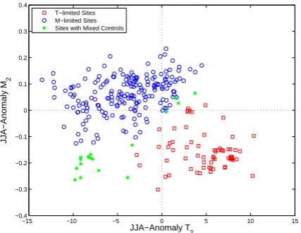
The point estimates of the parameters cluster in anomaly-parameter space according to each site’s classification as temperature-limited, moisture-limited, or mixed-control sites (Fig. 8). The estimated values ofT1fall below the mean
lo-cal JJA temperature (not shown). In other words, the mean summer temperatures all fall above the threshold for nonzero growth at every site, which is consistent with the fact that the chronologies we used at these locations were in fact sam-pled from living trees. Data at sites classified as temperature-sensitive constrain all estimates of T2 to values above the
mean local summer temperature. Summer temperature varia-tions therefore influence modeled growth at these sites. Sites classified as moisture-limited or as having mixed controls tend to have values ofT2that fall below local summer mean
temperatures; thus temperature variability will have less of an effect on modeled growth. The results for the moisture parameters are similar. All sites have calibrated values ofM1
falling below the climatological mean soil moisture content, so that there is enough moisture for modeled growth to occur across the experimental domain in summer. Calibrated values ofM2are greater than local climatological mean soil
mois-ture for all sites classified as moismois-ture-limited, but mixed-control and temperature-limited sites tend to have values of
−15 −10 −5 0 5 10 15 −0.4
−0.3 −0.2 −0.1 0 0.1 0.2 0.3 0.4
JJA−Anomaly T
2
JJA−Anomaly M
2
T−limited Sites M−limited Sites Sites with Mixed Controls
Fig. 8. Plot of estimatedM2versus estimatedT2at each site, with
both parameters measured as anomalies relative to the local clima-tological mean summer temperature. The color of points denotes the classification of the controls on modeled growth at each site.x=0 andy=0 define the mean local summer temperature and soil mois-ture content, respectively.
Given that the parameter estimates of the lower thresholds
T1 andM1 fall below mean summer climatological values
at all sites, the distribution of the anomaly point estimates inT2×M2 space contains the most information about the
modeled climate controls on growth (Fig. 8). In the sec-ond quadrant of the plot (defined by anomaly T2<0 and
anomalyM2>0 one would expect sites where moisture
gen-erally limits summer growth, since climatological temper-atures tend to fall above the optimal temperature growth limit, but soil moisture tends to fall below its optimal growth limit. All of the sites whose parameterizations end up in this quadrant are in fact classified as moisture-limited by our classification scheme. The fourth quadrant (anomalyT2>0,
anomalyM2<0) would seem to define a region of
parame-ter space describing temperature-limited growth, and indeed the sites whose estimated parameters are in this quadrant are nearly all classified this way. The sites that fall into quadrant III and far from the quadrant boundaries are mixed-control sites, as one would expect for locations where trees are sen-sitive to both variations in summer moisture and temperature variability.
The modeled climate controls on growth break the con-tinental United States into roughly three regions. In both the pseudoproxy and observed proxy experiments, the north-west contains mainly temperature-controlled sites (red mark-ers in quadrant IV of Fig. 8), while moisture-controlled sites fill the west and midwest (blue markers in quadrant II of Fig. 8), and mixed-control sites are most common in the southeast and along the eastern seaboard (green markers in quadrant III Fig. 8). This pattern is generally consistent with our knowledge of the climate sensitivity of the North Amer-ican tree-ring network (e.g., Meko et al., 1993).
The point estimates ofT2 andM2 derived from the
sci-entifically based priors described here are generally similar in value to those derived from uniform priors (Supplement Fig. 3). This result is consistent with the fact that the ratios of posterior to prior variance for these parameters tend to be ap-preciably less than one at most sites, thus indicating that the posteriors are dominated by information from the data. By contrast, estimates ofT1andM1tend to differ more
appre-ciably, but the associated posterior to prior variance ratios for these parameters are close to one. In general, the difference in the point estimates tends to be greatest where the data in-form the posteriors least, while sites with high learning (and hence posterior-to-prior variance ratios close to zero) exhibit little difference in posteriors derived from either prior (Sup-plement Fig. 4).
4 Discussion
The Bayesian inference scheme is skillful in recovering the known parameters used to create pseudoproxy ring-width se-ries. Although real-world analogs to the pseudoproxy target model parameters may not be known, the skill in the pseudo-proxy context supports the notion that the approach will esti-mate parameters that optimize VS-Lite’s fit to observed tree-ring width chronologies. The results of the PPE and OPMC are similar in terms of their spatial distributions of the mod-eled controls on growth, as well as the model sensitivities to the growth response parameters. These correspondences further support the applicability of pseudoproxy experiment results to studies using observed proxy data. The skill of ob-served ring-width index simulations is also shown to improve after calibrating the parameters, as compared to simulations run with parameter values set to the prior medians.
In addition to point estimates of the parameters, the spread of the posterior distributions also provides measures of the estimation uncertainty and the model sensitivity to the pa-rameters. We find that the VS-Lite model is generally least (most) sensitive to the value ofM1(M2), as the ratio of
pos-terior to prior variance is very close to one (zero) at all sites in both pseudoproxy and observed proxy experiments (Figs. 3 and 5). The model sensitivity to the temperature thresholds
T1andT2depends on the particular site.
faith in the representation of the underlying science and its inherent uncertainty reflected in the prior distributions. Our publicly available code includes flexible options for users to define their own priors, should new information from future field studies of tree growth render the default set of priors described here obsolete.
The choice of finite support or range is another component of prior specification that may heavily influence the posterior inference, as in the case of the parameterM2at most sites
in this study. The posterior distributions of this parameter at most sites show high probability mass toward the upper bound of the compact prior support (see Fig. 1 and bottom right panel of Fig. 4), indicating that the data alone imply val-ues of this parameter above the region allowed by the prior. However, the upper limit of the prior represents a physical constraint on biological thresholds for optimal moisture con-ditions for plant growth, as excessive soil moisture values may become detrimental to plant growth (Kozlowski, 1984). Given that the modeling of soil moisture within VS-Lite is known to be simplistic (Tolwinski-Ward et al., 2011), we be-lieve the posteriors here represent an objective compromise between the data and prior knowledge of the parameter, given the uncertainty of VS-Lite.
The location of parameter point estimates relative to lo-cal climatologilo-cal means in multidimensional anomaly pa-rameter space presents a graphical tool for understanding the climate controls on the modeled ring width signal (Fig. 8). At sites where VS-Lite reasonably represents growth, this type of plot could help identify and predict changes in the climate–proxy relationship that result from climatic nonsta-tionarities driving mean environmental conditions across bi-ological thresholds. In such cases of “divergence” (D’Arrigo et al., 2004; Carrer and Urbinati, 2006), one would expect the point representing the optimal set of parameter choices to cross from one quadrant into another after the climatic shift. At any site where the VS-Lite model fits the associated observed chronology well, the proximity of the parameters fitted by the present methodology to the boundaries between quadrants in Fig. 8 might be used to diagnose the potential for calibration–interval relationships between ring-width and climate to degrade under past shifts in climatology, and thus provide an important diagnostic before a given ring-width series is used for climate reconstruction. The spread of pa-rameter ensemble members produced by our estimation tech-nique could even be used in a Monte Carlo sense to quan-tify the probability that, for instance, a chronology character-ized by temperature-limited growth in the calibration interval “crosses the line” into a moisture-limited, mixed-control, or complacent growth response regime for a shift in climatology of a given number of degrees and volumetric soil moisture content.
This approach may be particularly valuable for reconstruc-tions that combine information contained in ring-width se-ries with that from other proxy sources. Currently, the pa-rameter estimation scheme is in use for probabilistic
recon-structions of paleoclimate from tree-ring width data and co-located isotopic dendrochronologies; preliminary results are sketched by Evans et al. (2013), and details are in prepa-ration by Tolwinski-Ward et al. (2013). At the southwest-ern American site in question, the ring-width variations dis-play strong moisture sensitivity during the calibration inter-val; however, the isotopic data suggest an anomalously wet interval in the pre-instrumental period. The reconstruction employs a Bayesian hierarchical model in which VS-Lite is used to link the variations in the proxy data to past variations in temperature and moisture. In that setting, the parameter-estimation procedure explored here is used to derive an en-semble of parameters consistent with the VS-Lite model and observed tree-ring width indices during a calibration inter-val. As described above in discussion of Fig. 8, the draws of the parameter values from the posterior allow for quantifica-tion of the probability that ring-width growth was insensitive to hydroclimatic variability during the reconstruction inter-val due to a general increase in available moisture resources indicated by the isotopic data.
5 Conclusions
The Bayesian calibration scheme presented here skillfully recovers parameter estimates near the values used to create synthetic tree-ring width data. The spread of the posterior distributions shows that the model fit to data is generally sensitive (insensitive) to the value of the moisture threshold
M2 (M1), and may or may not be sensitive to the
tempera-ture threshold parameters depending on location. Estimates of the VS-Lite model’s uncertainty provided by the scheme appear to be robust outside of the interval used for calibra-tion. The location of estimated parameters relative to local climatology in multidimensional parameter space provides insight into the climate controls on modeled tree-ring growth, and may also provide information about the potential for in-stability in the calibration–interval climate–ring-width rela-tionships before the instrumental record. The output of the estimation procedure enables users of VS-Lite to represent fully the range of model error stemming from uncertainty in its parameterization in both forward simulations of tree-ring width and inverse paleoclimate estimation settings.
Supplementary material related to this article is available online at: http://www.clim-past.net/9/1481/ 2013/cp-9-1481-2013-supplement.zip.
Acknowledgements. This work was supported in part by an Amer-ican Association of University Women Dissertation Fellowship and grants NSF ATM-0724802, NSF ATM-0902715, NSF DMS-1204892, and NOAA NA060OAR4310115. Malcolm Hughes lent disciplinary expertise to help with prior elicitation. Tom Kennedy and Walt Piegorsch provided comments on technical aspects of sampling and sensitivity analysis, and Doug Nychka provided insight that helped refine the discussion. We thank the contributors to the International Tree-Ring Data Bank, IGBP PAGES/World Data Center for Paleoclimatology, NOAA/NCDC Paleoclimatology Program, Boulder, Colorado, USA, for making their chronologies available, Chris Daly and the PRISM project for making their work freely available, and Benno Blumenthal for making the PRISM data easily accessible on the IRI Data Library. The comments and suggestions of two anonymous reviewers greatly assisted us in clarifying the writing and improving the substance of the evidence presented.
Edited by: J. Guiot
References
Boreux, J.-J., Naveau, P., Guin, O., Perreault, L., and Bernier, J.: Extracting a common high frequency signal from Northern Que-bec black spruce tree-rings with a Bayesian hierarchical model, Clim. Past, 5, 607–613, doi:10.5194/cp-5-607-2009, 2009. Carrer, M. and Urbinati, C.: Long-term change in the sensitivity of
tree-ring growth to climate forcing in Larix decidua, New Phy-tol., 170, 861–872, 2006.
Carrer, M., Anfodillo, T., Urbinati, C., and Carraro, V.: High altitude forest trees sensitivity to global warming: results from long-term and short-term analyses in the Italian Eastern Alps, in: The im-pacts of Climate variability on Forests. Lecture Notes in Earth Sciences, 74, edited by: Beniston, M. and Innes, J. L., 171–189, Springer, Berlin, Germany, 1998.
Chib, S. and Greenberg, E.: Markov Chain Monte Carlo Simulation Methods in Econometrics, Economet. Theor., 12, 409–431, 1996. Chiles, J. and Delfiner, P.: Geostatistics: Modeling Spatial Uncer-tainty, Wiley Series in Probability and Statistics, New York, NY, 1999.
Cook, E., Meko, D., Stahle, D., and Cleaveland, M.: Drought re-constructions for the continental United States, J. Climate, 12, 1145–1162, 1999.
Daly, C., Halbleib, M., Smith, J., Gibson, W., Doggett, M., Tay-lor, G., Curtis, J., and Pasteris, P.: Physiographically sensitive mapping of climatological temperature and precipitation across the coterminous United States, Int. J. Climatol., 28, 2031–2064, doi:10.1002/joc.1688, 2008.
D’Arrigo, R. D., Kaufmann, R. K., Davi, N., Jacoby, G. C., Laskowski, C., Myneni, R. B., and Cherubini, P.: Thresholds for warming-induced growth decline at elevational tree line in the Yukon Territory, Canada, Global Biogeochem. Cy., 18, GB3021, doi:10.1029/2004GB002249, 2004.
Deslauriers, A., Rossi, S., Anfodillo, T., and Saracino, A.: Cambial phenology, wood formation and temperature thresholds in two contrasting years at high altitude in southern Italy, Tree Physiol., (Oxford, UK), 28, 863–871, 2008.
Evans, M., Kaplan, A., and Cane, M.: Pacific sea surface temperature field reconstruction from coral δ18O data using reduced space objective analysis, Paleoceanography, 17, 1, doi:10.1029/2000PA000590, 2002.
Evans, M. N., Tolwinski-Ward, S. E., Thompson, D. M., and An-chukaitis, K. J.: Applications of proxy system modeling in high resolution paleoclimatology, Quaternary Sci. Rev., 76, 16–28, doi:10.1016/j.quascirev.2013.05.024, 2013.
Fritts, H. C.: Tree Rings and Climate, The Blackburn Press, New York, 2001.
Fritts, H. C., Shashkin, A., and Downes, G.: A Simulation Model of Conifer ring growth and cell structure, in: Tree Ring Analysis, edited by: Wimmer, R. and Vetter, R., Chap. 1, 3–32, Cambridge University Press, Cambridge, UK, 1999.
Garfinkel, H. and Brubaker, L.: Modern climate–tree-growth rela-tionships and climatic reconstruction in sub-Arctic Alaska, Na-ture, 286, 872–874, doi:10.1038/286872a0, 1980.
Gaucherel, C., Campillo, F., Misson, L., Guiot, J., and Boreux, J.: Comparison of a process-based tree-growth model: Comparison of optimization, MCMC, and Particle Filtering algorithms, Env-iron. Modell. Softw., 23, 1280–1288, 2008.
Gelman, A. and Rubin, D.: Inference from Iterative Simula-tion Using Multiple Sequences, Statist. Sci., 7, 457–472, doi:10.1214/ss/1177011136, 1992.
Gelman, A., Carlin, J., Stern, H., and Rubin, D.: Bayesian Data Analysis, Chapman and Hall, Boca Raton, Florida, 2003. Gilks, W., Richardson, S., and Spiegelhalter, D. (Eds.): Markov
Chain Monte Carlo in Practice, Chapman and Hall, Boca Raton, FL, 1996.
Ecol., 97, 57–66, 2009.
Huang, J., van den Dool, H. M., and Georgakakos, K. P.: Analysis of model-calculated soil moisture over the United States (1931– 1993) and applications to long-range temperature forecasts, J. Climate, 9, 1350–1362, 1996.
K¨orner, C.: Winter crop growth at low temperature may hold the answer for alpine treeline formation, Plant Ecol. Div., 1, 3–11, 2008.
K¨orner, C.: Alpine treelines: functional ecology of the global high elevation tree limits, Switzerland: Springer Basel, 2012. K¨orner, C. and Hoch, G.: A Test of treeline theory on a
mon-tane permafrost island, Arct. Antarct. Alp. Re., 38, 113–119, doi:10.1657/1523-0430(2006)038[0113:ATOTTO]2.0.CO;2, 2007.
K¨orner, C. and Paulsen, J.: A world-wide study of high altitude treeline temperatures, J. Biogeogr., 31, 713–732, doi:10.1111/j.1365-2699.2003.01043.x, 2004.
Kozlowski, T.: Responses of woody plants to flooding, in: Flooding and Plant Growth, edited by: Kozlowski, T., 129–163, Academic Press, New York, 1984.
Mann, M. E., Zhang, Z., Hughes, M. K., Bradley, R. S., Miller, S. K., Rutherford, S., and Ni, F.: Proxy-based reconstructions of hemispheric and global surface temperature variations over the past two millennia, Proc. Nat. Acad. Sci. USA, 105, 13252– 13257, doi:10.1073/pnas.0805721105, 2008.
Meko, D., Cook, E. R., Stahle, D. W., Stockton, C. W., and Hughes, M. K.: Spatial Patterns Of Tree-Growth Anomalies In The United States And Southeastern Canada, J. Climate, 6, 1773–1786, 1993.
Misson, L.: MAIDEN: a model for analyzing ecosystem pro-cesses in dendroecology, Can. J. For. Res., 34, 874–887, doi:10.1139/x03-252, 2004.
Misson, L., Rathgerber, C., and Guiot, J.: Dendroecological analysis of climatic effects on Quercus petraea and Pinus halepensis radial growth using the process-based MAIDEN model, Can. J. For. Res., 34, 888–898, doi:10.1139/x03-253, 2004.
Robert, C.: The Bayesian Choice: From Decision-Theoretic Foun-dations fo Computational Implementation, Springer Texts in Statistics, Paris, 2007.
Rossi, S., Deslauriers, A., Anfodillo, T., and Carraro, V.: Evidence of threshold temperatures for xylogenesis in conifers at high altitudes, Oecologia, 152, 1432–1939, doi:10.1007/s00442-006-0625-7, 2007.
Shumway, R. and Stoffer, D.: Time Series Analysis and Its Appli-cations, Springer Texts in Statistics, New York, NY, 2006. Smerdon, J.: Climate models as a test bed for climate
reconstruc-tion methods: pseudoproxy experiments, WIREs Clim. Change, 3, 63–77, doi:10.1002/wcc.149, 2012.
Taylor, W. P.: Significance of Extreme or Intermittent Conditions in Distribution of Species and Management of Natural Resources, with a Restatement of Liebig’s Law of Minimum, Ecology, 15, 374–379, 1934.
Tolwinski-Ward, S. E., Evans, M. N., Hughes, M. K., and An-chukaitis, K. J.: An efficient forward model of the climate con-trols on interannual variation in tree-ring width, Clim. Dynam., 36, 2419–2439, doi:10.1007/s00382-010-0945-5, 2011. Tolwinski-Ward, S. E., Tingley, M. P., Nychka, D. W., Evans, M. N.,
Hughes, M. K., and Leavitt, S. W.: Probabilistic reconstructions of local temperature and soil moisture from potentially nonsta-tionary tree-ring width data, in preparation, 2013.
Tukey, J.: The Collected Works of John W. Tukey, Volune IV Phi-losophy and Principles of Data Analysis: 1965–1986, Wadsworth & Brooks/Cole Advanced Books, Statistics/Probability Series, Murray Hill, New Jersey, 1986.
Vaganov, E. A., Hughes, M. K., and Shashkin, A. V.: Growth dynamics of conifer tree rings: Images of past and future environments, Ecol. Studies 183, Springer-Verlag, Berlin/Heidelberg/New York, 2006.
Vaganov, E. A., Anchukaitis, K. J., and Evans, M. N.: How well understood are the processes that create dendroclimatic records? A mechanistic model of climatic control on conifer tree-ring growth dynamics, in: Dendroclimatology: Progress and Prospects, edited by: Hughes, M., Swetnam, T., and Diaz, H., Developments in Paleoecological Research, Chap. 3, Springer-Verlag, Dordrecht, Netherlands, 2011.