www.atmos-meas-tech.net/9/491/2016/ doi:10.5194/amt-9-491-2016
© Author(s) 2016. CC Attribution 3.0 License.
EARLINET Single Calculus Chain – technical – Part 1:
Pre-processing of raw lidar data
Giuseppe D’Amico1, Aldo Amodeo1, Ina Mattis2,4, Volker Freudenthaler3, and Gelsomina Pappalardo1
1Consiglio Nazionale delle Ricerche, Istituto di Metodologie per l’Analisi Ambientale (CNR-IMAA), Tito Scalo, Potenza, Italy
2Leibniz Institute for Tropospheric Research, Leipzig, Germany
3Ludwig-Maximilians-Universität, Meteorologisches Institut Experimentelle Meteorologie, Munich, Germany 4Deutscher Wetterdienst, Meteorologisches Observatorium Hohenpeißenberg, Germany
Correspondence to: Giuseppe D’Amico ([email protected])
Received: 28 July 2015 – Published in Atmos. Meas. Tech. Discuss.: 7 October 2015 Revised: 23 December 2015 – Accepted: 2 February 2016 – Published: 12 February 2016
Abstract. In this paper we describe an automatic tool for the pre-processing of aerosol lidar data called ELPP (EAR-LINET Lidar Pre-Processor). It is one of two calculus mod-ules of the EARLINET Single Calculus Chain (SCC), the au-tomatic tool for the analysis of EARLINET data. ELPP is an open source module that executes instrumental corrections and data handling of the raw lidar signals, making the lidar data ready to be processed by the optical retrieval algorithms. According to the specific lidar configuration, ELPP automat-ically performs dead-time correction, atmospheric and elec-tronic background subtraction, gluing of lidar signals, and trigger-delay correction. Moreover, the signal-to-noise ratio of the pre-processed signals can be improved by means of configurable time integration of the raw signals and/or spa-tial smoothing. ELPP delivers the statistical uncertainties of the final products by means of error propagation or Monte Carlo simulations.
During the development of ELPP, particular attention has been payed to make the tool flexible enough to handle all lidar configurations currently used within the EARLINET community. Moreover, it has been designed in a modular way to allow an easy extension to lidar configurations not yet im-plemented.
The primary goal of ELPP is to enable the application of quality-assured procedures in the lidar data analysis starting from the raw lidar data. This provides the added value of full traceability of each delivered lidar product.
Several tests have been performed to check the proper functioning of ELPP. The whole SCC has been tested with
the same synthetic data sets, which were used for the EAR-LINET algorithm inter-comparison exercise. ELPP has been successfully employed for the automatic near-real-time pre-processing of the raw lidar data measured during several EARLINET inter-comparison campaigns as well as during intense field campaigns.
1 Introduction
Lidar networks like EARLINET (European Aerosol Re-search LIdar NETwork) are powerful tools to investigate the role of the aerosols in a large number of important at-mospheric processes (Pappalardo et al., 2014). They can perform coordinated measurements of the vertical profile of aerosol-related optical parameters with high vertical and temporal resolution. Coordinated lidar networks provide ob-servations covering continental and global scales, which al-low studies of the long-range transport of aerosol, the estab-lishment of climatologies over large geographical scales, and large-scale monitoring of special events.
One of these tools is the Single Calculus Chain (SCC), a flex-ible chain of software modules for the automatic analysis of lidar data. A general overview of the SCC is provided by D’Amico et al. (2015). This paper describes ELPP (EAR-LINET Lidar Pre-Processor), which is the SCC module for the automatic pre-processing of the raw lidar data. The SCC module for the retrieval of aerosol optical properties from the pre-processed data is called ELDA (EARLINET Lidar Data Analyzer) and is described in detail by Mattis et al. (2016). The implementation of ELPP as a unified pre-processor mod-ule has been mainly triggered by the heterogeneity of the EARLINET lidar systems. Moreover, ELPP provides a way to standardize all of the instrumental corrections, and the data handling which must be applied to the raw lidar data before they can be used as input for the optical retrieval module. This is fundamental for the application of a rigorous qual-ity assurance program on the lidar data analysis, in which all of the analysis steps starting from the raw lidar data up to the final lidar products (including pre-processing procedures) should be included.
The paper is structured in three main sections. Section 2 describes in detail ELPP. More technical aspects are covered in Sect. 2.1. The main features of the implemented proce-dures are summarized in Sect. 2.2. The algorithm for the au-tomatic gluing of lidar signals is reported in Sect. 2.3. A de-scription of the error propagation is provided in Sect. 2.4. Finally, the validation of ELPP and the conclusions are in Sects. 3 and 4, respectively.
2 EARLINET Lidar Pre-Processor (ELPP)
The typical SCC analysis scheme comprises two steps (D’Amico et al., 2015): the pre-processing of raw data with ELPP and the subsequent optical processing of the pre-processed lidar data with ELDA. ELPP is based on open source software, and it will be made available on-request to anyone interested to contribute in the development.
By “pre-processing” we mean the set of operations, which must be applied to the raw lidar data before they can be pro-cessed by ELDA. ELPP is designed to operate on the li-dar data measured by all of the EARLINET lili-dar systems in a fully automatic way. This is made possible by register-ing all instrumental parameters needed for the pre-processregister-ing in a centralized SCC database (D’Amico et al., 2015), where this information is structured in terms of lidar configurations. Each single lidar system can be linked to several lidar con-figurations, which describe different lidar set-ups with spe-cialized measurement capabilities (for example day-time or night-time conditions). When a raw measurement is submit-ted to the SCC, a corresponding entry is creasubmit-ted in the SCC database linking the measurement session to the lidar config-uration to be used for the analysis. According to that, the raw lidar data are handled and corrected for instrumental effects to provide pre-processed signals that, once saved on a local
storage, can be directly managed by the SCC optical process-ing module ELDA. The automatic procedures implemented in ELPP do not require the interaction of a human operator to run and to produce the final results. This is a fundamen-tal point in the effort to minimize the manpower needed to perform lidar analysis and consequently to improve the near-real-time availability of the lidar data at network level.
ELPP has been developed as a very flexible and expand-able tool: many different lidar configurations can be pre-processed using ELPP in different ways. This is made pos-sible by introducing the concept of SCC usecases. In sum-mary, a usecase represents a procedure to deliver a particular aerosol product like aerosol extinction or backscatter coef-ficient profiles. Usecases select specific retrieval schemes to calculate the corresponding optical products in both the pre-processing and the optical pre-processing analysis modules. As it will be discussed in Sect. 2.2, each lidar configuration is con-nected to the retrieval of a specific set of aerosol products. The way in which each product is retrieved is determined by a specific usecase according to the lidar configuration char-acteristics. The aerosol backscatter coefficient, for example, must be retrieved in different ways depending on the num-ber and the type of available lidar channels. That means, the raw elastic and corresponding nitrogen Raman signals need to be handled in a different way if they are split, for example, in near- and far-range channels, or not. From ELPP develop-ment point of view, the impledevelop-mentation of the SCC usecases required the identification of all pre-processing procedures and instrumental corrections adopted within the EARLINET community. All these procedures and corrections were criti-cally evaluated and finally implemented in ELPP, which en-ables the usage of this tool by all EARLINET systems. More details about SCC usecase are discussed in D’Amico et al. (2015), where a list of all implemented usecases is reported in the Appendix.
The modular structure of ELPP permits an easy imple-mentation of new usecases and thereby the use of ELPP and of the SCC for new EARLINET systems, non-EARLINET systems, and for other lidar networks independent of EAR-LINET. As a consequence, ELPP plays an important role in making the SCC extensible in more general frameworks like, for example, GALION (GAW Aerosol LIdar Observa-tion Network) as well as in naObserva-tional lidar networks. Typically, in such networks the optical processing retrieval algorithms are the same (or very similar to the) ones used within EAR-LINET, but lidar experimental configurations may change significantly.
Web interface Daemon
Database ELDA
Storage ELPP
SCC input files SCC intermediate files
SCC output files
SCC server
Raw data provider
SCC input files
SCC intermediate files
Figure 1. Block structure of the Single Calculus Chain.
has all of the information necessary to fully utilize and to evaluate the product, and it is easy to perform a consistent re-analysis of any data set keeping trace of the history of the analyses made.
Moreover, ELPP provides the possibility to check the qual-ity of all corrections and data handling procedures. The im-plementation of quality-certified procedures on both pre-processing and pre-processing levels (Böckmann et al., 2004; Pappalardo et al., 2004; Freudenthaler et al., 2016) allows the application of a rigorous and homogeneous quality as-surance program for the data measured by lidars with differ-ent instrumdiffer-ental characteristics. This is particularly impor-tant for a network like EARLINET, where the standardiza-tion of aerosol optical products is a fundamental requirement. ELPP is also an important tool for the long-term sustain-ability of the SCC. While lidar systems in the research com-munity are often upgraded with new channels or new detec-tion capabilities, ELPP, acting as the interface between the hardware level and the optical retrievals, delivers the pre-processed signals always in the same format. This allows the analysis of the data of a new lidar without modifying any of the other SCC modules.
In the next sub-section we describe the technical aspects of ELPP including its requirements and its different interfaces. After that, in Sect. 2.2, a description of the implemented al-gorithms will be provided specifying the procedures and the parameters that can be configured for the pre-processing of raw lidar data.
2.1 ELPP technical aspects
ELPP is a command line tool developed in ANSI C. It can be compiled using any C compiler, which is compatible with ANSI C, such as the freely available GNU Compiler
Collec-tion GCC (https://gcc.gnu.org/). The GCC can be used on both 32 and 64 bit environments for a quite large number of processor families and on many popular operating sys-tems like Linux, Unix, Mac OS, and Windows. As ELPP is developed in C, its source code can be implemented on any platform supported by the GCC without any recoding. The main requirements of ELPP are a MySQL database (http://www.mysql.com) and the NetCDF C libraries (http:// www.unidata.ucar.edu/software/netcdf/). All of the files used and generated by the SCC are in NetCDF format.
ELPP can be operated as a SCC module and also as a stand-alone module.
When it is used as a SCC module, it is automatically started by a further module (SCC daemon) whenever nec-essary. Figure 1 shows the general structure of the SCC and also the role played by ELPP in the automatic analysis of raw lidar data.
If used as a stand-alone module, the ELPP executable re-quires some mandatory command line parameters; i.e. the measurement ID of the lidar observation, that should be pre-processed, and the name of the MySQL database contain-ing all of the instrumental parameters needed by the pre-processing phase. As an optional command line parameter the name of a configuration file can be provided, which con-tains, for example, the path of the input, output, and log files. ELPP provides a user-configurable logging system, which produces a log file for each analyzed measurement.
The module ingests a NetCDF file containing a time series of raw lidar data to be analyzed. Raw time series correspond-ing to different lidar channels can be included in one scorrespond-ingle input file. The raw lidar data set is a three-dimensional array with the dimensions measurement time, channel, and range bin. It is fundamental that this array contains the raw lidar data as measured and without any modification. In particu-lar, the photon-counting signals should be provided in counts (positive integer numbers) while the analog signals should be provided in mV (real numbers). If the lidar acquisition system provides photon-counting and/or analog raw signals in different units, they need to be converted. The conversion must be applied by the raw data provider before submitting the data to the SCC. As different data acquisition systems provide the raw lidar data in different units, which might even change with system versions, it is not possible to in-clude this conversion step in the SCC. ELPP checks if the photon-counting raw profiles have been submitted using the required units, and if not, the corresponding raw data file is not accepted for the analysis. A further check on theoretical maximum count rate is performed in applying the dead-time corrections as reported in Sect. 2.2.1.
number of laser shots accumulated for each signal profile, the laser pointing angles, the measurement ID, and other similar parameters. The parameters, which are not related to the in-dividual measurement but to the lidar configuration, like the laser repetition rate, the emitted and detected wavelengths, the channels acquisition mode, and so on, are retrieved from the SCC database. To retrieve the full set of the SCC database parameters relevant for a specific raw data set, each single measurement (i.e. each single NetCDF input file) gets regis-tered in the database, and it is associated to an alpha-numeric string (i.e. measurement ID) which is defined in NetCDF in-put file. To assure a one-to-one correspondence between each raw data set and the corresponding measurement ID string, it is not allowed to submit NetCDF input file with a surement ID already present in the database. Using the mea-surement ID in appropriate database queries, it is possible to retrieve all information needed for the analysis of a spe-cific measurement which is not included in the corresponding NetCDF input file.
The raw data provider should decide how many raw lidar profiles to be included in a single input file taking into ac-count different aspects. The total size of a single NetCDF input file should be less than 200–300 MB to ensure a stable uploading on the SCC server. The maximum time length of a single NetCDF file also depends on the availability of ancil-lary information to be used in the analysis (i.e. radio sound-ing profiles, overlap correction functions). Each NetCDF in-put file can be linked to one specific set of ancillary data sets, which are used for the analysis of the whole time series. If, for example, there are four radio soundings per day avail-able for a certain site, the maximum time length of a single NetCDF input file is 6 h.
The cloud screening is another important operation to be applied to the lidar data before the submission to the SCC. The quality of the SCC optical products can not be as-sured, if there are signatures of low-level clouds in the raw lidar time series. As a consequence, individual lidar pro-files contaminated by low-level clouds should not be in-cluded in the NetCDF input file. A new module implement-ing a fully automatic cloud maskimplement-ing on high resolution li-dar data is under development, and it will be included in the SCC in the framework of the ACTRIS-2 (Aerosol, Clouds and Trace gases Research InfraStructure Network) projects (http://www.actris.eu).
As already mentioned, it is possible to provide other kinds of input files to ELPP together with the raw data NetCDF input file, i.e. a file containing pressure and temperature pro-files provided by a radio sounding to be used for the calcula-tion of the signal backscattered by atmospheric molecules (as explained in Sect. 2.2.4), a file containing the overlap correc-tion funccorrec-tion, and a file consisting of the lidar-ratio profile to be used in the retrieval of the particle backscatter coef-ficient using elastic-only techniques. Even if these two last files typically are not needed in the pre-processing phase, ELPP interpolates them at the same vertical resolution of the
pre-processed data and saves the corresponding interpolated data in new files. In particular, ELDA is designed to use these files for the retrieval of the aerosol optical properties.
The output files of ELPP are in NetCDF format and con-tain the pre-processed, range-corrected signals, the so called intermediate files, which were handled according to all anal-ysis steps reported in Sect. 2.2. Table 1 summarizes the de-scription of all NetCDF variables used to identify differ-ent types of pre-processed signals in output files. For in-stance, the total elastic range-corrected signal is represented by the variable elT, the atmospheric nitrogen vibrational– rotational Raman range-corrected signal by vrRN2. The range-corrected signal for the near range and for the far range are represented by variables whose names contain the “nr” or “fr” string, respectively. Selecting appropriate usecases, it is possible to specify whether gluing procedures should be performed by ELPP gluing the raw signals, or by ELDA gluing the optical products. The products calculated from near-range and far-range pre-processed signals are the ones for which ELDA gluing has been selected by the raw data provider (Mattis et al., 2016). All of the NetCDF variables reported in Table 1 are bi-dimensional arrays with dimen-sions time and range bin. The time and vertical resolutions of these arrays are specified in the SCC database for each product as explained in the next section. Moreover, as the products are defined in the SCC database for a single emis-sion wavelength (i.e. aerosol extinction coefficient at 355 nm or aerosol backscatter coefficient at 1064 nm), each interme-diate file refers always to a single wavelength.
Other information included in the ELPP output files is the molecular extinction and the molecular atmospheric trans-mission profiles, the range resolution and the vertical reso-lution, the number of averaged laser shots, and so on. All parameters for the optical retrieval, which are provided by the user in the input NetCDF file, are directly transferred to ELDA within the header of the intermediate files.
The input parameters needed for the analysis of the lidar data are retrieved from the header of the NetCDF file or, if not provided in the file header, from a relational MySQL database (SCC database) with general values for a certain lidar system configuration. The structure of this database is described in D’Amico et al. (2015) in Sect. 3.1.
Once ELPP has been started, it is possible to monitor the status of the pprocessing using its return values. ELPP re-turns a null value if the pre-processing was successfully per-formed and positive integer values in case any error occurred. Each return value is associated to a specific type of error, such as a failure in gluing the lidar signals or an inconsis-tency in the definition of the variables in the raw input file, to provide detailed information about the problem occurred. 2.2 Description of implemented algorithms
Table 1. Description of different types of pre-processed, range-corrected signals delivered by ELPP and the corresponding NetCDF variable name in the ELPP output files. All of the variables refer to a single emission wavelength. As a consequence, pre-processed data corresponding to different wavelengths are saved in separate files.
Pre-processed range-corrected signal NetCDF variable name
Elastic total backscattered signal elT
Perpendicular∗polarization component of the total backscattered signal elCP
Parallel∗polarization component of the total backscattered signal elPP
Vibrational–rotational Raman backscattered signal by nitrogen molecules vrRN2
Near-range elastic total backscattered signal elTnr
Near-range perpendicular∗polarization component of the total backscattered signal elCPnr Near-range parallel∗polarization component of the total backscattered signal elPPnr Near-range vibrational–rotational Raman backscattered signal by nitrogen molecules vrRN2nr
Far-range elastic total backscattered signal elTfr
Far-range perpendicular∗polarization component of the total backscattered signal elCPfr Far-range parallel∗polarization component of the total backscattered signal elPPfr Far-range vibrational–rotational Raman backscattered signal by nitrogen molecules vrRN2fr
∗With respect to the linear polarization state of the incident laser beam.
known and well described in the literature. For this reason the related relevant literature is mentioned in the following sub-sections without providing detailed descriptions of the implemented formulas. On the other hand, details of the im-plementation and user adjustable parameters are explained. The implementation of the automatic algorithm for the glu-ing of lidar signals is discussed in greater detail in Sect. 2.3. As already mentioned in the previous section, ELPP re-quires the presence of a MySQL database where the char-acteristics of the analysis to be performed are specified. In particular, starting from a measurement ID passed to ELPP via the command line, it is possible to retrieve from the database all required information such as how many products should be calculated (Np in Fig. 2), how many lidar
chan-nels are needed for the calculation of each product (Nc(p)
with 0< p≤Np), the full set of the input parameters needed
for the analysis (dead-time value, trigger delay, etc.), and the name of the data file containing the raw input time series cor-responding to all lidar channels linked to the measurement ID to analyze.
Once this information is obtained, ELPP starts to calcu-late pre-processed signals for all configured products. There are two main loops involved in the pre-processing chain: an external loop on the products to be calculated (index p in Fig. 2 with p=1, . . ., Np), and an internal loop in which
all the product-related channels are pre-processed sequen-tially (index c with c=1, . . ., Nc(p)). The pre-processing
steps performed to calculate a specific set of optical prod-ucts can be illustrated by means of a practical example. Let us suppose two products – (Np=2) the aerosol backscatter
coefficient (product p=1) and the aerosol extinction coef-ficient (p=2), which should be calculated for a particular measurement ID by using two elastic channels at 355 nm (elTnr, elTfr) – and two vibrational–rotational N2 Raman channels at 387 nm (vrRN2nr, vrRN2fr). To calculate the
aerosol backscatter coefficient the channels elTnr (channel
c=1), elTfr (c=2), vrRN2nr (c=3) and vrRN2fr (c=4) are needed soNc(1)=4. Let us also suppose the two
Measurement ID Get info from SCC DB
Npproducts Nc(p)lidar channels
Pre-processing parameters Raw filename
Read input file
setp= 1
Calculation productp
setc= 1
Read raw time series of channelc
Analog N Y Dead-time correction Subtract background (atmospheric and/or elect.)
Trigger-delay corr.
Time integration
c=c+ 1
c≤Nc(p)
Y N Glue Y N Vertical smoothing Overlap correction Range correction Mol. Rayleigh-scatt. calculation Write output p=p+ 1
p≤Np
N Y Stop Gluing
Figure 2. ELPP work flow. ELPP gets the full set of information and parameters needed for the pre-processing of a specific measure-ment ID performing suitable queries to the SCC database. This set includes how many products should be calculated (Np), how many lidar channels are needed for the calculation of each product (Nc(p) with 0< p≤Np), all input parameters required for the analysis (dead-time value, trigger delay, etc.), and the name of the input NetCDF file corresponding to the selected measurement ID. There are two main loops involved in the pre-processing chain: an external loop on the products to be calculated (indexp) and an internal loop in which all of the product-related channels are pre-processed se-quentially (indexc). The operations performed by the single blocks are described in the text. A single output file (intermediate NetCDF file) is generated for each product.
elTfr and the gluing of vrRN2nr with vrRN2fr. After this step, ELPP completes the calculation of the current product performing the operations reported on the right part of Fig. 2. Optionally a vertical smoothing of pre-processed lidar sig-nals is performed. Typically, smoothing is done to increase the SNR of the pre-processed signals. Different smoothing options can be selected, like linear, polynomial, and nat-ural cubic spline (Press et al., 2007). Moreover, the sig-nals are range-corrected and optionally corrected for incom-plete overlap. Finally, the molecular contribution to the at-mospheric extinction and transmissivity are calculated at the same resolution of pre-processed lidar signals as described in Sect. 2.2.4. The pre-processed signals are then stored in
a specific intermediate NetCDF file. This file will be used as input by the ELDA module (D’Amico et al., 2015; Mattis et al., 2016) to retrieve the aerosol backscatter product. In the specific case of the example above, this file contains the time series of the elastic (N2Raman) glued pre-processed signals under the variable elT (vrRN2).
Once the pre-processing corresponding to the first uct is ended, ELPP switches to the next scheduled prod-uct (p=2) which is, according to the example above, the aerosol extinction coefficient. The procedure is very similar to the one already described for the aerosol backscatter coef-ficient. The only difference is that for this product there are only two signals to be pre-processed (vrRN2nr and vrRN2fr,
Nc(2)=2) and only one gluing needs to be performed. The
results are stored in another intermediate NetCDF file which contains the time series of the N2Raman glued pre-processed signals under the variable vrRN2. ELDA will use this file to retrieve the aerosol extinction coefficient profile.
2.2.1 Dead-time correction
The dead-time correction of photon-counting signals is non-linear. A typical lidar photon-counting channel consists of a photo-multiplier, which ideally generates an electrical pulse for each photon impacting its photo-cathode (event), a pulse discriminator to reduce the noise counts, and finally a fast counter to count the number of events in a fixed inter-val of time, the time bin. As each electrical pulse has a cer-tain width, two pulses closer to each other than about the pulse width can not be discriminated. The actual minimum time interval between two subsequently countable events, called dead-timeτ (Evans, 1955), depends on the setting of the pulse discriminator and on the counting electronics. The time corresponds to a maximum count rate. The dead-time causes a non-linearity between the actual intensity at the photo-multiplier photo-cathode and the counted events, which can be described theoretically by means of photon statistics. As the real processes are not ideal, the mathemati-cal correction of the non-linearity works only in first approx-imation. Furthermore, there are two models to describe the counting characteristic of a photon-counter, i.e. the paralyz-able and the non-paralyzparalyz-able model. A paralyzparalyz-able count-ing system is not able to provide a second output count if a timeτ is not elapsed after the previous pulse. Moreover, if an additional pulse arrives within the dead-timeτ, the actual dead-time of the system is further extended byτ. In this way, at high count rate, the unit is unable to respond, it is “par-alyzed”, and the count-rate output is 0. In contrast, a non-paralyzable counter outputs counts at maximum count rate as long as subsequent photon pulses are not discriminable. ELPP includes optionally both models for dead-time correc-tion (in first approximacorrec-tion). The formulas used by the SCC to correct for dead-time are the following (Evans, 1955):
cm=
cr 1+τ cr
, (2)
where cm andcr are the measured and the real count rate, respectively. The Eq. (1) refers to a paralyzable counter while the Eq. (2) is used if a non-paralyzable counter is assumed.
Once the dead-time valueτ and the model to use for the correction are provided to ELPP, the corresponding photon-counting lidar signal will be automatically corrected by solv-ing the Eqs. (1) or (2) for the unknown cr. The Eq. (1) is solved numerically in the interval [0,1/τ] using the well-known secant method (Press et al., 2007).
It is important to underline that the Eq. (1) can be solved only ifcmis less or at least equal to the absolute maximum of the exponential function on right-hand side. As a conse-quence, the following condition on the measured count rate has to be verified:
cm≤ 1
eτ, (3)
whereeis the Euler’s number.
For the non-paralyzable model, the correction for dead time is made by inverting Eq. (2):
cr=
cm 1−τ cm
. (4)
Ascr≥0 andcm≥0, the Eq. (4) can be solved only if the following condition on the measured count rate is valid:
cm< 1
τ. (5)
According to the selected model, the condition expressed by the Eqs. (3) or (5) is used as constraint on the actual val-ues of the photon-counting signals rejecting all the cases in which it is not verified.
As the dead-time correction is non-linear, it is applied as the first stage of the pre-processing procedure as shown in Fig. 2.
Here it should be mentioned that in general the reliabil-ity of dead-time correction decreases with increasing count-rate: both correction models reported above usually fail in reproducing the correct behaviour of a real counting sys-tem at high count-rates. As a consequence, each photon-counting lidar channel should be carefully adjusted to not ex-ceed a maximum count-rate (typically 10–30 MHz depend-ing on the value of τ) in all the range bins for which the photon-counting signal is supposed to be used.
The dead time of a photon-counting system can be eval-uated measuring the counting probability distribution gen-erated by a Poissonian source (like a tungsten lamp) as de-scribed in Johnson et al. (1966); Whiteman et al. (1992).
2.2.2 Trigger delay
In general, the data acquisition unit of a lidar system gets a trigger from the laser to start the signal recording. Due to the electronic circuits in the laser and in the data acquisition unit, there is always a delay between the outgoing laser pulse and the time at which the acquisition system actually starts to record the lidar profile. If this trigger delay is not properly taken into account, a systematic error is made in associat-ing each lidar range bin with the correspondassociat-ing atmospheric range. A delay, for example, of 100 ns induces a systematic shift of the atmospheric ranges of 15 m. This shift causes a systematic error in the range-correction of the lidar sig-nal, which propagates to the calculation of the final aerosol properties. The error is especially large for the aerosol extinc-tion coefficient calculated with the Raman method in the near range. The exact trigger delay can be measured and provided to ELPP as input parameter for each lidar channel (Freuden-thaler et al., 2016). If1T is the trigger delay of a particu-lar lidar channel and TS1=(t1,t2, . . . ,tn) is the time scale used by the acquisition system to sample the lidar profile, the actual lidar range scale is calculated from the delayed time scale TS2=(t1+1T,t2+1T, . . . ,tn+1T).
If different lidar channels have different trigger delays, ELPP interpolates all recorded lidar signals from the time scale TS2 (which may change from channel to channel) to the time scale TS1(which is the same for all channels). This operation enables the consistent calculation of the lidar prod-ucts for which multiple channels are needed.
It is possible to choose a linear or a natural cubic spline interpolation (Press et al., 2007). The preferred option is the linear interpolation as usually the trigger-delay correction re-quires only a time shift of lidar signals. As first step, for each valuetk of the time scale TS1 the closest higher and lower values of time scale TS2 are selected. Let us sup-pose these values are tl−1+1T and tl+1T respectively.
The value of the lidar signalStk intk is then determined by
the equation of the straight line passing through the points
(tl−1−1T , Stl−1−1T)and(tl−1T , Stl−1T)as follows:
Stk=Stl−1+1T +
Stl+1T−Stl−1+1T
1t (tk−tl−1−1T ), (6)
withtl−1+1T < tk≤tl+1Tand1t=tl−tl−1representing the lidar signal range bin width.
If the trigger delay is a multiple of the signal range bin width (1T =u1t ), the Eq. (6) is equivalent to a re-binning of the signal (Stl =Stl+u). For all the cases in which
The natural cubic spline interpolation option should be used only if an additional smoothing on lidar signals is re-quired.
2.2.3 Background subtraction
A raw lidar signalS(z, λ)can be expressed by Eq. (7),
S(z, λ)=Spar(z, λ)+Smol(z, λ)+Satm(λ)+Sel, (7) whereSpar(z, λ)andSmol(z, λ)are the signal contributions backscattered by particles (par) and molecules (mol) at alti-tudezand at wavelengthλ.Satm(λ)is the optical signal back-ground from the atmosphere, i.e. the sky brightness, which is independent of range, andSelrepresents the electronic signal background, which stems from electronic effects of the sig-nal detection and data acquisition.Selcan have a temporally constant part and a temporally changing part, i.e. changing with lidar range.
It is fundamental to removeSatm(λ)andSelfrom the mea-sured lidar profiles before applying any optical retrieval al-gorithm.
The amount of the constant background components
Satm(λ)+Selcan be determined either in the far range of the lidar signal, far enough that the expected contribution from atmospheric backscatter is negligible, or in the pre-trigger range before the laser pulse, where the signal must be free of electronic distortions, which could influence the determina-tion of the constant background. In both cases the constant background value is calculated as mean value over signal ranges, which are large enough so that the residual standard error of the mean is negligible.
ELPP implements both options for the calculation of the range-independent contribution in Eq. (7), i.e.
1. the mean of the lidar signal in the far-range region; 2. the mean of lidar signal in the pre-trigger region. The selection can be done in the SCC database or in the input file.
In the case of option 1, the minimum (zmin) and the maxi-mum (zmax) ranges (expressed in m) for the background cal-culation have to be provided in the raw data input file. ELPP estimates the background value from the mean and the cor-responding statistical uncertainty from the standard error of the mean of the lidar signal betweenzminandzmax.
In the case of option 2, three parameters are needed: a min-imum (imin) and a maximum (imax) range bin index in the pre-trigger region for the calculation of the background value and the uncertainty as above, and a first valid range bin index (i0) withi0≥imaxexplained in the following. After the back-ground value and the corresponding statistical uncertainty have been calculated, all points up to i0 are removed from the lidar signal, because they are not necessary for the fur-ther calculations. Then the background is subtracted from the lidar signal.
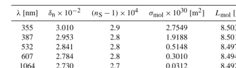
Table 2. Numerical values of the parameters involved in Eqs. (9) and (10) calculated for the most common lidar wavelengths accord-ing to Bucholtz (1995). The quantityδnrepresents the molecular
de-polarization factor for unpolarized (natural) incident light scattered at right angle,nS is the refractive index of standard air,Lmolthe
molecular lidar-ratio, andσmolthe total Rayleigh-scattering cross
section per molecule given by Eq. (9) whenρmol=1, and a value
ofρS=2.54743×1025m−3for the molecular number density for
standard air in Eq. (9) is assumed.
λ[nm] δn×10−2 (n
S−1)×104 σmol×1030[m2] Lmol[sr]
355 3.010 2.9 2.7549 8.503
387 2.953 2.8 1.9188 8.501
532 2.841 2.8 0.5148 8.497
607 2.784 2.8 0.3010 8.494
1064 2.730 2.7 0.0312 8.492
Temporally changing and hence range-dependent contri-butions in Sel are typically due to electronic distortions, which mainly affect the analog lidar signals. They can have temporally random components and components which are synchronal with the repetition of the laser pulse. While the random components zero out in the average of many subse-quent lidar signals, the synchronal components do not and can contribute a significant distortion to the lidar signal. The stationary synchronal components can be determined from so-called dark signals, which are measured, for example, with a fully obscured telescope so that no light from the at-mosphere reaches the detectors and only the distortions are left. The dark signals have to be averaged over a long enough time period in order to decrease the random contributions sufficiently. ELPP automatically subtracts a dark measure-ment from the lidar signal if the former is included in the SCC input file as single dark signal or as dark time series. If a dark time series is provided, an average dark profile is cal-culated automatically and subtracted from the lidar signals.
Both dark signal and background subtraction can be ap-plied together.
2.2.4 Molecular Rayleigh-scattering calculation
compressibility factor (Penndorf, 1957):
ρmol(z)=
P (z)
RT (z), (8)
whereRis the universal gas constant.
The temperature and pressure profiles are either calculated from a standard atmosphere model, or taken from the mea-surements of a close-by radiosounding that can be provided to the SCC as a separate input file. Once the molecular num-ber density is obtained, the calculation of the molecular op-tical parameters, i.e. the backscatter and extinction coeffi-cients, is done following the procedure reported in Bucholtz (1995) and Miles et al. (2001). In particular, the extinction coefficient (αmol), the lidar ratio (Lmol), and the atmospheric transmission (Tmol) are calculated using the following formu-las:
αmol(λ, z)= 24π3 λ4ρ2
S
n2S−1
n2S+2
!2
6+3δn 6−7δn
ρmol(z) (9)
Lmol(λ)= 8π
3
1+δn
2
(10)
Tmol(λ, z)=exp
−
z/cosθ
Z
0
αmol(λ, ξ ) dξ
cosθ
, (11)
where λis the wavelength (in cm), z is the altitude above the lidar station, andθis the zenith angle of the lidar point-ing. The other quantities, which are the molecular number density for standard air (ρS), the molecular depolarization ra-tio for unpolarized (natural) incident light scattered at right angle (δn), and the refractive index of standard air (nS), are calculated according to Bucholtz (1995). The integral in the Eq. (11) is computed numerically using the trapezoidal rule (Press et al., 2007). The numerical values of the parameters involved in the Eqs. (9) and (10) calculated for the most com-mon lidar wavelengths are reported in Table 2. ELPP writes in its output file the quantities given by the Eqs. (9) and (10), and the atmospheric transmission given by Eq. (11) at both emission and detection wavelengths.
2.3 Gluing
Lidar signals can cover a quite large dynamic range, because the intensity of the light backscattered from the aerosol-laden boundary layer in the near range (e.g. at 0.5 km altitude) is several orders of magnitudes higher than the intensity of the light backscattered from the rather clean troposphere (e.g. at 10 km altitude). As it is demanding to cover this large dy-namic range with one data acquisition channel with linear response, several approaches are used to overcome this prob-lem.
One option is to split the signal output from a single photo-multiplier into two signals and to record one signal using ana-log detection mode and the other with the photon-counting
technique (Whiteman et al., 2006; Newsom et al., 2009). The analog signal provides good performance for the strong backscatter from the near range but suffers from the high analog noise and distortions in the far range. In contrast, the photon-counting signal is saturated in the near range but pro-vides a good performance in the far range. Therefore it is ap-propriate to use the analog for the near-range signalSn and the photon-counting for the far-range signalSf.
Another option is to split the lidar signal optically using a beam splitter and to detect the split components with two detectors and subsequent data acquisitions. Both signals are attenuated, if necessary, with neutral density filters to match the dynamic range of the data acquisitions for the stronger near-range and the weaker far-range signal. In general, the photon-counting technique is used for both signals due to its superior performance regarding detection linearity compared to analog detection.
A third option is to use two (or more) telescopes with sep-arate detection electronics, i.e. one small telescope designed to detect the near-range signal and the other larger telescope optimized to measure the weak far-range signal.
In either case, the complementary signals need to be glued to get a single “extended” lidar signal for the signal analysis (Whiteman et al., 2006; Newsom et al., 2009; Walker et al., 2014).
Before gluing, the near-range and the far-range signals need to be screened for low-level clouds, corrected for in-strumental effects like dead time, trigger delay, etc., and the backgrounds have to be subtracted as explained above.
For the first two options the signals are glued by ELPP and then analyzed by ELDA as one signal. Typically, if there are lidar configurations with multiple telescopes, the gluing is made by ELDA at product levels (Mattis et al., 2016) .
ELPP contains a fully automatic algorithm for the gluing of analog and photon-counting signals as well as for the glu-ing of two photon-countglu-ing signals. The algorithm is divided in three main parts. The procedure starts with the determi-nation of a first guess of the gluing region as described in Sect. 2.3.1. After that, the algorithm optimizes the gluing re-gion performing statistical tests as illustrated in Sect. 2.3.2. Finally, the signals are glued in the optimal gluing region as reported in Sect. 2.3.3.
2.3.1 First guess of the gluing region
Slope test Stability test m,n,Δz,rth
z0,z1,Sn,Sf
N=points in[z0, z1]
N <15
N Y Stop rlinear corr. ofSnandSf within[z0, z1]
r < rth Y N Stop i= 1,j= 0
z 0=z0
z 1=z1
points inN
I= [z 0, z1]
N <5 Y
N j= 1
Y
N
zi= 0,j= 1 0=z0+jΔz
z 1=z1−iΔz
N≤30
N YSLinear fitf=KSn inI
KSRn−=Sf
inI
Linear fit
R=kz
inI
|k|< mΔk
N
Y
S=KSn
SplitIin
I1=I2
Linear fit
Sf=KSn inI1andI2
|K1−K2|< nΔK2
1+ ΔK2 2 N Y z
0,z1,K,ΔK
z
0=z0+ Δz
z 1=z1−Δz
SLinear fitf=KSn inI
SplitIin
I1=I2
Linear fit
Sf=KSn inI1andI2
R= KSn−Sf inI1andI2
Linear fitR=kz
inI1andI2
|k1−k2|< mΔk2
1+ Δk2 2
N
Y
z
0=z0+jΔz
z 1=z1−iΔz
Figure 3. Work flow diagram of the automatic algorithm for the glu-ing of near-range and far-range lidar signals implemented in ELPP.
an analog or a photon-counting signal. Analog signals are in general measured using pre-amplifiers with several input ranges. Each input range is characterized by a minimum level below which signal distortions and/or the signal noise be-come significant. This minimum level, which is used to deter-mine the upper altitude (z1) of the gluing region, is expressed by the ratioS/F whereS is the maximum detectable input signal level andF is a parameter characterizing the analog to digital converter (ADC). If we assume, for example, the ADC output is reliable only for values larger thanNrestimes its resolution we obtain
F =2 nb−1
Nres
, (12)
wherenbis the number of the bits of the ADC. The values of the parameterF can be defined in the system configura-tion for each channel. If the near-range signal is detected in
photon-counting mode, the upper altitudez1is determined by setting a lower threshold for the SNR.
2.3.2 Optimal gluing region
Starting from the values ofz0andz1determined in the pre-vious section, ELPP tries to optimize the gluing region using the automatic algorithm shown in Fig. 3. Besidesz0andz1, the algorithm requires the following input data provided in the input file and in the SCC database, which are explained in detail later:
– the near-range and far-range signalsSnandSf, respec-tively;
– a thresholdrthfor the linear correlation ofSnandSf; – the step1zwith which the gluing region is decreased
during the iterations;
– the statistical uncertainty limits to evaluate the slope test and the stability test given in number of standard devia-tionsmandn, respectively.
First, the algorithm determines the number of range binsN
betweenz0andz1. If this number is less than 15, the gluing region is considered too small to perform a reliable gluing and consequently the gluing is not done. IfNis larger than or equal to 15, the linear correlationrof the signalsSnandSfis calculated betweenz0andz1. AsSnandSfshould be highly linear correlated in the gluing region, only regions wherer
is larger than the thresholdrth (typically 0.9) are accepted; otherwise the gluing is not performed.
Ifr≥rth, a further investigation of the gluing region is done in order to exclude parts of the region with significant deviations between the two signals and to minimize the glu-ing error. This is made by changglu-ing iteratively the region
[z0, z1] until the signalsSn andSf are consistent according to the additional tests described below. This procedure is il-lustrated by the block “Slope test” in Fig. 3.
In the optimal gluing region the signalsSnandSfshould coincide, even in the fine structure due to aerosol layers and photon noise, and only differ due to the different electronic noise sources with zero means and slopes. To investigate this the following steps are carried out:
– the signalSn is normalized to the signalSfin the glu-ing region. This is done performglu-ing the least square re-gressionSf=KSn in the gluing region, and using the obtainedKto normalize the signalSn;
– the residualsR=KSn−Sfare calculated in the gluing region;
If the signalsSn andSf are statistically equivalent in the gluing region, the values of the slopekshould not be signif-icantly different than 0, and the residualsR should be nor-mally distributed around a null mean value. This condition is considered verified if the absolute value ofkis smaller than
mstandard deviations (default 2) of the slope resulting from the least square fit.
If the gluing range is large (e.g. if the number of range bins in the gluing range is greater than 30), there could be a dif-ference between the first and the second half of the gluing range. In this case we introduce a constraint on the absolute value of the curvatureC of the residuals, which is estimated from the difference of the slopes of the residuals of the first and the second half of the gluing range (C= |k1−k2|). The condition is met if
C < m1C, (13)
where 1C=
q
1k12+1k22. The integer m represents the level of confidence of the Eq. (13) as exclusive condition. For a Gaussian distribution and form=1, there is about the 32 % of probability the two slopes (k1andk2) agree (in statis-tical sense) even if the Eq. (13) is not verified (Taylor, 1997). Form=2 the same probability is reduced to about 5 %.
Figure 3 (block “slope test”) shows the work flow of the optimization of the gluing region. The starting gluing region
[z0, z1]is changed until the slope test described above is sat-isfied. First the algorithm tries to iteratively reducez1in steps of1zwhile keepingz0fixed. In Fig. 3 this phase starts with settingi=1 andj=0. In each iteration the slope test is eval-uated: if the test is passed, the current region is used as op-timal gluing region; if it is not passed,z1is further reduced by1z. If there is no region in which the slope test is passed, the algorithm starts to increase iterativelyz0in steps of1z while keepingz1fixed at its starting value (i=0 andj=1 in Fig. 3). If no region can be found passing the slope test, the gluing is not done.
If a gluing region has passed the slope test, the stability test is further applied, which is shown by the block “stability test” of Fig. 3. The region, which has passed the slope test, is divided into two equal subregions, and in each of these sub-regions the signal Sn is normalized to the signal Sf, which results in two signalsS1=K1SnandS2=K2Sn, whereK1 andK2are the two slopes obtained from the two least squares line fits. If the gluing region is chosen in a proper way,S1and
S2are indistinguishable taking into account the correspond-ing signal uncertainties. To test this, the followcorrespond-ing condition (stability test) is evaluated:
|K1−K2|< n
q
1K12+1K22, (14) where1K1and1K2are the standard deviations onK1and
K2 obtained from the two least squares line fits, and n is a positive integer (default value is 1) having the same sta-tistical meaning of the integermin the Eq. (13). If the con-dition expressed by the Eq. (14) is met, we assume that the
selected interval is the optimal gluing region, otherwise the interval is progressively reduced increasing (decreasing) the lower (higher) border in step of1zuntil the stability test is verified.
2.3.3 Signals combination
If the gluing algorithm described in the previous section ends successfully, the optimal gluing region is returned (z00 and
z01) together with the normalization gluing factorKused to normalize the signalSnand the corresponding error1K re-sulting from the least square line fit. Finally, the signalsSn andSfare glued calculating first the quantityS0n=KSnand then calculating the gluing point (zg) as the range bin, within the optimal gluing region, that minimizes the square differ-ences of the signalSn0 andSf. The glued signalS(z)and the corresponding statistical error1S(z)are the following:
S(z)=
(
KSn(z), ifz < zg;
Sf(z), otherwise;
(15)
1S(z)=
(p
(K1Sn)2+(Sn1K)2, ifz < zg;
1Sf(z), otherwise.
(16)
An example of the application of this algorithm to real li-dar data is shown in Fig. 4. The algorithm is applied to the analog (near range) and photon-counting (far range) elastic cross-polarized signals measured by the EARLINET refer-ence system MUSA (MUlti-wavelength System for Aerosol, Madonna et al., 2011). The blue curve (upper plot) is the photon-counting elastic cross signal at 532 nm summed-up over 1 h, which is used as far-range signal. The first-guess gluing region is indicated as regionAin Fig. 4, i.e. between
z0=2445 m andz1=3917 m, and the red curve represents the analog elastic cross signal at 532 nm normalized to the photon-counting signal in region A.
The region indicated with B (extending from 2445 up to 3097 m) is the region in which the slope test has passed, and region C (z00=2651 m andz01=2891 m) represents the opti-mal gluing region after the stability test. Region G is used to finally glue the signals. The green curve in Fig. 4 is the same as the red but normalized in region G.
0.1 1 10 100 1000
Count rate [MHz]
A
B
G
Gluing
Near-range rescaled (first guess) Near-range rescaled Far-range
-0.1 0 0.1 0.2
0 1000 2000 3000 4000 5000
Rel. diff.
Altitude [m]
Figure 4. Example of the results of the automatic gluing algorithm shown in Fig. 3. The algorithm is applied to the analog (near range) and photon-counting (far range) elastic cross signals measured at 532 nm by the MUSA lidar of the Potenza station. In blue is shown the photon-counting signal, in red the near-range signal normalized to the photon-counting signal in regionA, i.e. the first guess of the gluing region, and in green the near-range signal normalized in regionG, i.e. the final optimal gluing region. RegionBrepresents the gluing region obtained after the slope test shown in Fig. 3 and discussed in the text. “Gluing” marks the point at which the blue and green signals are glued. In the bottom plot the relative differences of the two rescaled analog signals with respect to the photon-counting profile are shown.
2.4 Error propagation
ELPP propagates the statistical errors in all steps shown in Fig. 2. Two different propagation methods are implemented: one based on the standard formula of statistical error propa-gation (Taylor, 1997), and another one based on Monte Carlo simulations (Robert and Casella, 2004), which is only used when the standard error propagation is not possible or too complex. This is the case, for example, if the interpolation or smoothing routines implemented in ELPP have been applied. The details of the application of the Monte Carlo method to the error propagation are given in Amodeo et al. (2016). In this section only the basic concepts are briefly discussed. Ifsi is either a raw or a processed lidar profile,1si the
cor-responding error profile, andF a generic operator we want to apply tosi (for example a smoothing procedure or a
fil-ter) to obtainSi=F(si), the Monte Carlo method offers an
efficient and general procedure to calculate1Si, i.e. the
un-certainty ofSi. The basic assumption is that eachsi is a mean
value with an uncertainty width1siaccording to a statistical
distribution. The first step consists of randomly varying all valuessi considering their1si as standard deviations. ELPP
assumes that analog signals are governed by Gaussian statis-tic and photon-counting signals follow Poissonian statisstatis-tic. In this way a new synthetic lidar signalsi0 can be generated
according to the assumed probability distribution and a cor-responding transformed signalSi0=F(si0)can be calculated. Repeating this procedure a statistically meaningful number of times, the error profile1Si can be estimated calculating
the standard deviation of theSi0. ELPP uses a default value of 30 variations ofSi0=F(s0i), which has been found to offer the best trade off between the calculation time needed and the accuracy of the retrieved errors. Optionally, the number of Monte Carlo variations can be also specified in the SCC database for each product.
The random extractor routine implemented in ELPP is based on a so-called Lehmer random number generator which returns a pseudo-random number uniformly dis-tributed in the interval 0.0 and 1.0 (Park and Miller, 1988). This uniform distribution is then mapped in Poissonian or Gaussian one (Odeh and Evans, 1974).
On the contrary, the evaluation of the statistical error cor-responding to each single raw signal range bin in the case of analog signals is not so trivial. For Gaussian distributions the standard deviation can not be inferred from the mean value like for the Poissonian case. To overcome this difficulty two options are implemented in ELPP.
The first consists of the possibility to provide, along with the raw analog signal time series, the corresponding statisti-cal error time series. This option is applicable only for sys-tems which are able to measure such kind of values e.g. by storing not only the mean values but also the sum of the square values. In this case the error of analog time series is propagated in all the operational blocks shown in Fig. 2 using the standard propagation formula or the Monte Carlo method.
If the statistical error time series are not provided, ELPP calculates the statistical errors of analog signals only after the time averaging (block “time integration” in Fig. 2) as the standard error of the mean of each range-bin value. In all the operations made before the time integration (i.e. background subtraction and trigger-delay correction) the error of analog signals is not propagated due to the difficulty to estimate the statistical error of analog signals without other information. In this case, the analog signal time series (Sha) and the corre-sponding standard errors (1Sha) after the time integration are calculated according to the following equations:
Sha(z)= 1
N
N (h+1)−1
X
j=N h
sja(z) (17)
1Sah(z)=
v u u t
PN (h+1)−1
j=N h
h
sja(z)−Sha(z)i2
N (N−1) (18) h≤ Nt−N
N , (19)
wheresja(z)is the analog time series before the time integra-tion withj=0, . . ., Nt−1, andN is the number of the raw
profiles belonging to the same time window (defined as the larger integer smaller than the ratio of the integration time window width and the raw time resolution ofsja(z)time se-ries).
To summarize, the statistical error of analog signals, if not provided directly by the raw data submitter, are first esti-mated using Eq. (18) during the “time integration” stage and then propagated in all the subsequent blocks shown Fig. 2.
Finally, in the case of photon-counting detection mode, the signal time series (Shp) and the corresponding standard errors (1Shp) after the time integration are calculated using the fol-lowing equations:
Shp(z)=
N (h+1)−1
X
j=N h
sjp(z) (20)
1Shp(z)=
v u u t
N (h+1)−1
X
j=N h
h
1sjp(z)i
2
, (21)
wheresjp(z)and1sjp(z)are the photon-counting time series and corresponding statistical error before the time integration (j=0, . . ., Nt−1).
3 Applications and validation
ELPP has been intensively tested with both synthetic and real lidar data to evaluate its performance under different condi-tions.
The synthetic data set used for testing is the same as used for the algorithm inter-comparison exercise performed in EARLINET (Pappalardo et al., 2004). The data set con-tains a 30 min time series of synthetic raw lidar signals sim-ulated under realistic experimental and atmospheric condi-tions. Both elastic and N2Raman raw lidar signals are taken into account to reproduce as much as possible a real measure-ment sample of a typical advanced multi-wavelength Raman lidar. The synthetic raw data were converted to SCC format and then submitted to and processed by the SCC. Finally, the performance of the whole SCC (ELPP and ELDA mod-ules) was evaluated comparing the retrieved optical profiles with the original input profiles. The results of this compari-son are discussed in details in Mattis et al. (2016). Here we just point out that all extinction and backscatter profiles re-trieved by the SCC from the inter-comparison data set are in good agreement with the input profiles.
0 2 4 6 8 10 12 14
108 109
Altitude [km]
RCS @ 355nm [A.U.]
RALI MARTHA PollyXT MSTL-2 MUSA
0 2 4 6 8 10 12 14
108 109
Altitude [km]
RCS @ 532nm [A.U.]
0 2 4 6 8 10 12 14
109 1010
Altitude [km]
RCS @ 387nm [A.U.]
0 2 4 6 8 10 12 14
109 1010
Altitude [km]
RCS @ 607nm [A.U.]
0 2 4 6 8 10 12 14
108 109 1010
Altitude [km]
RCS @ 1064nm [A.U.]
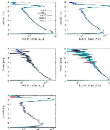
Figure 5. Range-corrected by ELPP for five lidar systems participating in the EARLI09 inter-comparison campaign (the same colour iden-tifies the same lidar system in all the plots). All profiles were taken from 21:00 to 23:00 UT on 25 May 2009. From left to right, upper panel: elastic-backscattered signals at 355 and 532 nm; middle panel: N2Raman backscattered signals at 387 and 607 nm; bottom panel:
elastic-backscattered signals at 1064 nm. The dotted grey curves represent the signals backscattered by atmospheric molecules computed using a close radiosounding. All signals are normalized in the atmospheric region between 9.5 and 10.5 km, which is assumed to be aerosol free.
To evaluate the SCC performance in analyzing raw data measured by different lidar systems, D’Amico et al. (2015) considered the EARLI09 session taken on 25 May 2009 from 21:00–23:00 UT for which a comparison among the SCC op-tical products (aerosol backscatter and extinction coefficient profiles) and the corresponding manually retrieved ones is reported. A subset of five EARLI09 participating systems has been selected on the basis of instrumental differences and representativeness within EARLINET comprising the following lidar systems: the Multi-wavelength Raman Lidar
plots in the middle panel show the nitrogen inelastic Ra-man range-corrected signals at 387 and 607 nm. In the bot-tom panel the elastic-backscattered range-corrected signals at 1064 nm are plotted. In all plots the molecular signals com-puted by ELPP from a correlative radiosounding are shown (grey dotted line). All range-corrected signals and the calcu-lated molecular backscattered signals have been normalized in the atmospheric region below the cirrus (9.5–10.5 km), which is assumed to be aerosol free. Figure 5 shows the advantages in using ELPP in a lidar inter-comparison cam-paign: the discrepancies between the range-corrected signals generated by ELPP for different lidar systems can be eas-ily estimated and evaluated. As a consequence, instrumental problems can be quickly detected and the causative misalign-ments or defects can be fixed. For instance, by using the pro-files plotted in Fig. 5, it is possible to select valid and reliable altitude ranges for each channel of each participating instru-ment (Wandinger et al., 2015).
ELPP has been also successfully used to provide near-real-time pre-processed lidar signals ready to be assimilated in air-quality models. An example of this application is given by the intense period of coordinated measurements performed in July 2012 by 11 EARLINET systems in the Mediterranean area. During this campaign, 72 h of continuous lidar mea-surements were carried out by all participating systems, and the aerosol products were calculated automatically by the SCC in terms of both pre-processed data and backscatter and extinction profiles were made available in near-real time (Sicard et al., 2015). The pre-processed signals generated by ELPP were assimilated in the air-quality model Polyphemus developed by Centre d’Enseignement et de Recherche en En-vironnment Atmosphérique (CEREA) allowing a better qual-ity of the PM10 and PM2.5 forecast on the ground (Wang et al., 2014).
4 Conclusions
ELPP, a fully automatic tool for the pre-processing of lidar data, was developed and extensively tested with both syn-thetic and real lidar data. It is a fundamental part of the EARLINET SCC because this calculus module generates the input files for the SCC optical processing module (ELDA) starting from raw lidar data. ELPP requires the presence of a MySQL database and of NetCDF libraries both free avail-able from Internet and can be also used as stand-alone mod-ule.
Depending on lidar configuration, ELPP applies differ-ent type of instrumdiffer-ental corrections and data handling pro-cedures on raw lidar data. The ELPP outputs are NetCDF files containing range-corrected signals ready to be used to retrieve optical parameters like aerosol extinction and/or backscatter coefficient profiles. The output files contain also profiles of atmospheric molecular parameters calculated from the standard model or from the correlative measurement
of pressure and temperature profiles at the same resolution of the range-corrected signals. This information is used by ELDA to retrieve optical results.
The key features of ELPP are the flexibility (it is possible to handle many different kinds of lidar configurations choos-ing among a quite large number of pre-defined options called usecases), the expandability (it is developed in a modular way, and it is relatively easy to add new system configura-tions not already covered), and finally it allows the applica-tion of a quality assurance program on lidar analysis includ-ing also the pre-processinclud-ing phase. Moreover all calculated products are fully traceable, and all metadata used to produce a specific product can be provided to allow its full evaluation. ELPP passed the test of EARLINET algorithm inter-comparison exercise providing results in good agreement with the expected ones. It was also extensively tested with real lidar data: during several EARLINET inter-comparison campaigns ELPP was used to provide pre-processed range-corrected signals of all the participating lidar systems in near-real time. As all corrections are made with the same ELPP procedures, the comparison of such pre-processed signals can be used to discover problems or distortions of the in-dividual lidar systems. Finally, the ability of ELPP to deliver pre-processed signals in near-real time during intense field campaigns was successfully tested during the EARLINET 72h operationally exercise performed by 11 Mediterranean EARLINET stations.
A new SCC module devoted to the automatic cloud mask-ing on the raw lidar data is under development and will be implemented in the SCC in the framework of the ACTRIS-2 project (http://www.actris.eu). A big improvement in the au-tomatism of both ELPP and the whole SCC is expected when this new module will be available.
We would like to point out that ELPP is open source, and that the procedures discussed in this paper are the first steps towards a fully automatic, robust, and flexible module for the pre-processing of lidar data. Improvements and enhance-ments from the lidar community are endorsed and promoted by the current developers.
Acknowledgements. The financial support for EARLINET in the
ACTRIS Research Infrastructure Project by the European Union’s Horizon 2020 research and innovation programme under grant agreement no 654169 and previously under the grants no. 262254 in the 7th Framework Programme (FP7/2007-2013) and no 025991 in the 6th Framework Programme (FP6/2002-2006) is gratefully acknowledged.
Edited by: A. Ansmann
References
I., Wagner, F., Rascado, J. L., Pereira, S., Lim, J., Ahn, J. Y., Tesche, M., and Stachlewska, I. S.: PollyNET: a network of mul-tiwavelength polarization Raman lidars, in: Proc. of SPIE, vol. 8894, Lidar Technologies, Techniques, and Measurements for Atmospheric Remote Sensing IX, International Society for Opti-cal Engineering, PO Box 10, Bellingham, WA 98227-0010 USA, 88940I–1–88940I–10, 2013.
Amodeo, A., D’Amico, G., Mattis, I., Freudenthaler, V., and Pap-palardo, G.: Error calculation for EARLINET products in the context of quality assurance and single calculus chain, Atmos. Meas. Tech. Discuss., in preparation, 2016.
Ansmann, A., Riebesell, M., and Weitcamp, C.: Measurement of atmospheric aerosol extinction profiles with a Raman lidar, Opt. Lett., 15, 746–748, 1990.
Ansmann, A., Riebesell, M., Wandinger, U., Weitcamp, C., Voss, E., Lahmann, W., and Michaelis, W.: Combined Raman elastic-backscatter lidar for vertical profiling of moisture, aerosol ex-tinction, backscatter and lidar ratio, Appl. Phys. B, 55, 18–28, 1992a.
Ansmann, A., Wandinger, U., Riebesell, M., Weitcamp, C., and Michaelis, W.: Independent measurement of extinction and backscatter profile in cirrus clouds by using a combined Raman elastic-backscatter lidar, Appl. Opt., 31, 7113–7131, 1992b. Böckmann, C., Wandinger, U., Ansmann, A., Bösenberg, J.,
Amiridis, V., Boselli, A., Delaval, A., De Tomasi, F., Frioud, M., Grigorov, I. V., Hågård, A., Horvat, M., Iarlori, M., Komguem, L., Kreipl, S., Larchevêque, G., Matthias, V., Papayannis, A., Pappalardo, G., Rocadenbosch, F., Rodrigues, J. A., Schneider, J., Shcherbakov, V., and Wiegner, M.: Aerosol lidar intercom-parison in the framework of the EARLINET project. 2. Aerosol backscatter algorithms, Appl. Opt., 43, 977–989, 2004. Bucholtz, A.: Rayleigh-scattering calculations for the terrestrial
at-mospehre, Appl. Opt., 34, 2765–2773, 1995.
Chaikovsky, A., Ivanov, A., Balin, Y., Elnikov, A., Tulinov, G., Plusnin, I., Bukin, O., and Chen, B.: Lidar network CIS-LiNet for monitoring aerosol and ozone in CIS regions, in: Proc. of SPIE, vol. 6160, Twelfth Joint International Symposium on At-mospheric and Ocean Optics/AtAt-mospheric Physics, International Society for Optical Engineering, P.O. Box 10, Bellingham, WA 98227-0010 USA, 616035–1–616035–9, 2006.
D’Amico, G., Amodeo, A., Baars, H., Binietoglou, I., Freuden-thaler, V., Mattis, I., Wandinger, U., and Pappalardo, G.: EAR-LINET Single Calculus Chain – overview on methodology and strategy, Atmos. Meas. Tech., 8, 4891–4916, doi:10.5194/amt-8-4891-2015, 2015.
Di Girolamo, P., Ambrico, P. F., Amodeo, A., Boselli, A., Pap-palardo, G., and Spinelli, N.: Aerosol Observations by Lidar in the Nocturnal Boundary Layer, Appl. Opt., 38, 4585–4595, 1999. Evans, R. D.: The Atomic Nucleus, McGrow-Hill, New York,
chap-ter 28, 785–794, 1955.
Fernald, F. G.: Analysis of atmospheric lidar observations: some comments, Appl. Optics, 23, 652–653, 1984.
Ferrare, R. A., Melfi, S. H., Whitemann, D. N., Evans, K. D., and Leifer, R.: Raman lidar measurements or aerosol extinction and backscattering: 1. Methods and comparisons, J. Geophys. Res., 103, 19663–19672, 1998.
Freudenthaler, V., Linné, H., Chaikovsky, A., Groß, S., and Rabus, D.: Internal quality assurance tools, Atmos. Meas. Tech. Dis-cuss., in preparation, 2016.
Johnson, F. A., Jones, R., McLean, T. P., and Pike, E. R.: Dead-Time Corrections to Photon Counting Distributions, Phys. Rev. Lett., 16, 589–592, 1966.
Klett, J. D.: Stable analytical inversion solution for processing lidar returns, Appl. Opt., 20, 211–220, 1981.
Madonna, F., Amodeo, A., Boselli, A., Cornacchia, C., Cuomo, V., D’Amico, G., Giunta, A., Mona, L., and Pappalardo, G.: CIAO: the CNR-IMAA advanced observatory for atmospheric research, Atmos. Meas. Tech., 4, 1191–1208, doi:10.5194/amt-4-1191-2011, 2011.
Mattis, I., Ansmann, A., Müller, D., Wandinger, U., and Althausen, D.: Multiyear aerosol observations with dual-wavelength Raman lidar in the framework of EARLINET, J. Geophys. Res., 109, D13203, doi:10.1029/2004JD004600, 2004.
Mattis, I., D’Amico, G., Madonna, F., Amodeo, A., and Baars, H.: EARLINET Single Calculus Chain – technical Part 2: Calcula-tion of optical products, Atmos. Meas. Tech. Discuss., in prepa-ration, 2016.
Miles, R. B., Lempert, W. R., and Forkey, J. N.: Laser Rayleigh scattering, Meas. Sci. Technol., 12, R33–R51, 2001.
Nemuc, A., Vasilescu, J., Talianu, C., Belegante, L., and Nicolae, D.: Assessment of aerosol’s mass concentrations from measured linear particle depolarization ratio (vertically resolved) and sim-ulations, Atmos. Meas. Tech., 6, 3243–3255, doi:10.5194/amt-6-3243-2013, 2013.
Newsom, R. K., Turner, D. D., Mielke, B., Clayton, M., Ferrare, R., and Sivaraman, C.: Simultaneous analog and photon counting detection for Raman lidar, Appl. Opt., 48, 3903–3914, 2009. Odeh, R. E. and Evans, J. O.: Algorithm AS 70: The Percentage
Points of the Normal Distribution, J. Roy. Stat. Soc. C-App., 23, 96–97, 1974.
Pappalardo, G., Amodeo, A., Pandolfi, M., Wandinger, U., Ans-mann, A., Bösenberg, J., Matthias, V., Amiridis, V., De Tomasi, F., Frioud, M., Iarlori, M., Komguem, L., Papayannis, A., Roca-denbosch, F., and Wang, X.: Aerosol lidar intercomparison in the framework of the EARLINET project. 3. Raman lidar algorithm for aerosol extinction, backscatter, and lidar ratio, Appl. Opt., 43, 5370–5385, 2004.
Pappalardo, G., Amodeo, A., Apituley, A., Comeron, A., Freuden-thaler, V., Linné, H., Ansmann, A., Bösenberg, J., D’Amico, G., Mattis, I., Mona, L., Wandinger, U., Amiridis, V., Alados-Arboledas, L., Nicolae, D., and Wiegner, M.: EARLINET: to-wards an advanced sustainable European aerosol lidar network, Atmos. Meas. Tech., 7, 2389–2409, doi:10.5194/amt-7-2389-2014, 2014.
Park, S. K. and Miller, K. W.: Random Number Generators: Good Ones Are Hard To Find, Commun. ACM, 31, 1192–1201, doi:10.1145/63039.63042, 1988.
Penndorf, R.: Tables of the refractive index for standard air and the Rayleigh scattering coefficient for the spectral region between 0.2 and 20.0µ and their application to atmospheric optics, J. Opt. Soc. Am., 47, 176–182, 1957.
Press, W. H., Teukolsky, S. A., Vetterling, W. T., and Flannery, B. P.: Numerical Recipes, The Art of Scientific Computing, Cambridge University Press, New York, NY, USA, 3 Edn., 2007.
Robert, C. and Casella, G.: Monte Carlo Statistical Methods, 2nd Edn., Springer-Verlag, New York, NY, USA, 2004.