University of Pennsylvania
ScholarlyCommons
Publicly Accessible Penn Dissertations
2018
Bayesian Model Selection And Estimation Without
Mcmc
Sameer Deshpande
University of Pennsylvania, [email protected]
Follow this and additional works at:
https://repository.upenn.edu/edissertations
Part of the
Statistics and Probability Commons
This paper is posted at ScholarlyCommons.https://repository.upenn.edu/edissertations/2953
For more information, please [email protected].
Recommended Citation
Bayesian Model Selection And Estimation Without Mcmc
Abstract
This dissertation explores Bayesian model selection and estimation in settings where the model space is too vast to rely on Markov Chain Monte Carlo for posterior calculation. First, we consider the problem of sparse multivariate linear regression, in which several correlated outcomes are simultaneously regressed onto a large set of covariates, where the goal is to estimate a sparse matrix of covariate effects and the sparse inverse covariance matrix of the residuals. We propose an Expectation-Conditional Maximization algorithm to target a single posterior mode. In simulation studies, we find that our algorithm outperforms other regularization competitors thanks to its adaptive Bayesian penalty mixing. In order to better quantify the posterior model uncertainty, we then describe a particle optimization procedure that targets several high-posterior probability models simultaneously. This procedure can be thought of as running several ``mutually aware'' mode-hunting trajectories that repel one another whenever they approach the same model. We demonstrate the utility of this method for fitting Gaussian mixture models and for identifying several promising partitions of spatially-referenced data. Using these identified partitions, we construct an approximation for posterior functionals that average out the uncertainty about the underlying partition. We find that our approximation has favorable estimation risk properties, which we study in greater detail in the context of partially exchangeable normal means. We conclude with several proposed refinements of our particle optimization strategy that encourage a wider exploration of the model space while still targeting high-posterior probability models.
Degree Type Dissertation
Degree Name
Doctor of Philosophy (PhD)
Graduate Group Statistics
First Advisor Edward I. George
Keywords
Bayesian hierarchical modeling, Clustering, Optimization, Spatial Smoothing, Variable Selection
BAYESIAN MODEL SELECTION AND ESTIMATION WITHOUT MCMC
Sameer K. Deshpande
A DISSERTATION
in
Statistics
For the Graduate Group in Managerial Science and Applied Economics
Presented to the Faculties of the University of Pennsylvania
in
Partial Fulfillment of the Requirements for the
Degree of Doctor of Philosophy
2018
Supervisor of Dissertation
Edward I. George, Universal Furniture Professor, Professor of Statistics
Graduate Group Chairperson
Catherine M. Schrand, Celia Z. Moh Professor of Accounting
Dissertation Committee
Dylan S. Small, Class of 1965 Wharton Professor, Professor of Statistics,
Abraham J. Wyner, Professor of Statistics
BAYESIAN MODEL SELECTION AND ESTIMATION WITHOUT MCMC
c
COPYRIGHT
2018
Sameer Kirtikumar Deshpande
This work is licensed under the
Creative Commons Attribution
NonCommercial-ShareAlike 3.0
License
To view a copy of this license, visit
Dedicated to my grandparents:
ACKNOWLEDGEMENT
First and foremost, I would like to thank my advisor Ed, for his constant support and
encouragement. No matter how busy you may have been, you have always taken time
to meet with me to discuss new ideas and problems. I have learned so much from our
discussions and always come away inspired to think about new directions. Most importantly,
however, through your example, you’ve shown me how to be a good colleague, mentor,
friend, and overall “good guy.” For that, I will be forever in your debt.
I would like to thank my committee members, Dylan, Adi, and Veronika. It has been such a
pleasure and honor working with each of you over the last several years. Thank you so much
for your constant inspiration and encouragement. I look forward to continued collaboration,
discussion, and friendship.
Thanks too to the entire Wharton Statistics Department for creating such a warm, familiar,
and welcoming environment. To the faculty with whom I have been lucky to interact – thank
you for your time, dedication, and so many stimulating conversations. To our incredible
staff – thank you for all that you do to keep our department running smoothly and for
making the department such a friendly place to work.
I have been blessed to have made so many incredible friends during my time at Wharton.
Matt and Colman – what an incredible journey it has been! Thank you for your constant
companionship these last five years. Raiden – it has been a real pleasure working with you
these last two years. I always look forward to our near-daily discussions, whether it is about
basketball or statistics. Gemma and Cecilia – I’ve loved getting to work with the two of
your over the last year and a half. While I am sad that our weekly “reading group” must
come to an end, I am so excited for many years of friendship and collaboration. I cannot
imagine what my time at Wharton would be like without each of you.
ABSTRACT
BAYESIAN MODEL SELECTION AND ESTIMATION WITHOUT MCMC
Sameer K. Deshpande
Edward I. George
This dissertation explores Bayesian model selection and estimation in settings where the
model space is too vast to rely on Markov Chain Monte Carlo for posterior calculation.
First, we consider the problem of sparse multivariate linear regression, in which several
correlated outcomes are simultaneously regressed onto a large set of covariates, where the
goal is to estimate a sparse matrix of covariate effects and the sparse inverse covariance
matrix of the residuals. We propose an Expectation-Conditional Maximization algorithm
to target a single posterior mode. In simulation studies, we find that our algorithm
outper-forms other regularization competitors thanks to its adaptive Bayesian penalty mixing. In
order to better quantify the posterior model uncertainty, we then describe a particle
opti-mization procedure that targets several high-posterior probability models simultaneously.
This procedure can be thought of as running several “mutually aware” mode-hunting
tra-jectories that repel one another whenever they approach the same model. We demonstrate
the utility of this method for fitting Gaussian mixture models and for identifying several
promising partitions of spatially-referenced data. Using these identified partitions, we
con-struct an approximation for posterior functionals that average out the uncertainty about
the underlying partition. We find that our approximation has favorable estimation risk
properties, which we study in greater detail in the context of partially exchangeable normal
means. We conclude with several proposed refinements of our particle optimization strategy
that encourage a wider exploration of the model space while still targeting high-posterior
TABLE OF CONTENTS
ACKNOWLEDGEMENT . . . iv
ABSTRACT . . . vi
LIST OF TABLES . . . ix
LIST OF ILLUSTRATIONS . . . x
CHAPTER 1 : Introduction . . . 1
CHAPTER 2 : The Multivariate Spike-and-Slab LASSO . . . 6
2.1 Introduction . . . 6
2.2 Model and Algorithm . . . 11
2.3 Dynamic Posterior Exploration . . . 18
2.4 Full Multivariate Analysis of the Football Safety Data . . . 33
2.5 Discussion . . . 39
CHAPTER 3 : A Particle Optimization Framework for Posterior Exploration . . . 41
3.1 Motivation . . . 41
3.2 A Variational Approximation . . . 42
3.3 Implementation . . . 44
3.4 Mixture Modeling with an Unknown Number of Mixture Components . . . 45
CHAPTER 4 : Identifying Spatial Clusters . . . 58
4.1 Model and Particle Search Strategy . . . 63
4.2 Simulated Example . . . 66
4.3 Discussion . . . 73
5.1 Whence Partial Exchangeability? . . . 74
5.2 A Multiple Shrinkage Estimator . . . 78
5.3 Approximate Multiple Shrinkage . . . 80
5.4 Towards a Better Understanding of Risk . . . 88
CHAPTER 6 : Conclusion and Future Directions . . . 96
6.1 Next Steps . . . 96
LIST OF TABLES
TABLE 1 : Low-dimensional variable selection and estimation performance . . 26
TABLE 2 : Low-dimensional covariance selection and estimation performance . 27
TABLE 3 : High-dimensional variable selection and estimation performance . . 28
TABLE 4 : High-dimensional covariance selection and estimation performance 29
TABLE 5 : Balance of covariates between football players and controls . . . 36
TABLE 6 : Risk comparison of smoothing within spatial clusters . . . 62
LIST OF ILLUSTRATIONS
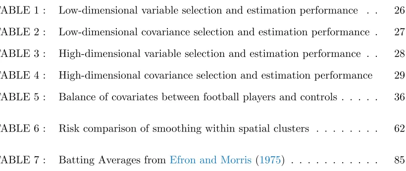
FIGURE 1 : Examples of spike-and-slab densities . . . 9
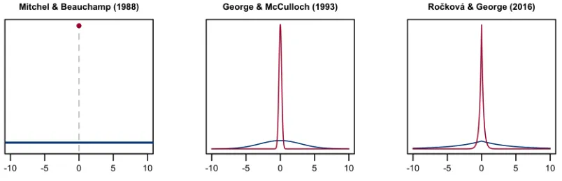
FIGURE 2 : Reproduction of Figure 2c inRoˇckov´a and George(2016) . . . 19
FIGURE 3 : Stability of the mSSL trajectories . . . 22
FIGURE 4 : Distributions of signal recovered and unrecovered by mSSL-DPE . 31 FIGURE 5 : Estimated residual graphical model in football safety study . . . . 38
FIGURE 6 : Gaussian mixture data . . . 54
FIGURE 7 : Partitions of the Gaussian mixture data . . . 55
FIGURE 8 : Log-counts of violent crime in Philadelphia . . . 60
FIGURE 9 : Three spatial partitions of the grid . . . 61
FIGURE 10 : Three specifications ofβ . . . 61
FIGURE 11 : Top nine spatial partitions when cluster means are well-separated 67 FIGURE 12 : Number of unique particles discovered . . . 68
FIGURE 13 : Risk of approximate estimator when clusters well-separated . . . . 69
FIGURE 14 : Top nine spatial partitions when the cluster means are not well-separated . . . 71
FIGURE 15 : Risk of approximate estimator when cluster means are not well-separated . . . 72
FIGURE 16 : Comparison of the standard and clustered Lindley estimators . . . 77
FIGURE 17 : Top four partitions . . . 82
FIGURE 18 : Risk of approximate multiple shrinkage estimator . . . 83
FIGURE 19 : Re-analysis ofEfron and Morris (1975)’s batting averages . . . 87
FIGURE 20 : Examples of perturbationsY+ . . . 94
CHAPTER 1 : Introduction
Given a realization of data, the Bayesian paradigm provides a coherent and tremendously
flexible framework within which to reason about our uncertainty about the data generating
process. A Bayesian analysis starts with a likelihood that is based on the distribution of
the data conditional on some unknown parameters, which are treated as random variables
drawn from apriordistribution. Together, the likelihood and prior are combined via Bayes’
rule to form theposterior distribution, which encapsulates all of our uncertainty about the
unknown parameters in light of the observed data. As Gelman et al. (2008) notes, this
specification of the likelihood is a “major stumbling block” for Bayesian analyses.
In this thesis, we consider situations where we have a combinatorially large number of
potential likelihoods (i.e. generative models) but are uncertain about which might be most
appropriate. We consider two general problems: model selection, in which we wish to
identify the models that best describe the data, and estimation of model-specific parameters
in the presence of this uncertainty. Conceptually, the Bayesian framework provides an easy
answer: simply place a prior over the collection of all models and turn the proverbial
Bayesian crank to compute the posterior. Moving from the joint distribution of the data
and generative model to the posterior requires computing the marginal likelihood for the
data. This in turn requires us to sum over the entire model space, which is often not
possible.
We focus on two problems where this is the case: multivariate linear regression and mixture
modeling. In multivariate linear regression, we aim to usepcovariates to predict the values
of q correlated outcomes simultaneously. When p and q are large and even greater than
the number of observations n, there is great interest in fitting sparse models, where only
a small number of covariates are used to predict each outcome and only a small number
of residuals are conditionally dependent on each other. Formally, this problem reduces to
covariances between the residuals. In all, there are 2pq+q(q−1)/2different combinations of the
supports of these two matrices, leading to a rather high-dimensional model space for even
moderately-sized p and q. For instance, in Section 2.4, we examine data from Deshpande
et al.(2017), an observational study on the long-term effects of playing high school football.
In that study, there werep= 204 covariates and q= 29 outcomes, yielding a model space of
dimension 26332 >101903.Clearly, we cannot expect to explore even a small fraction of this
space within a reasonable number of MCMC iterations. Next, we consider clustering and
mixture modeling, in which we assume each data point arose from one of several different
distributions. A priori, the number of mixture components and the allocation of each
observation to a component is unknown. We may encode this structure with a partition of
the integers [n] = {1,2, . . . , n}. In this problem, the dimension of our model space grows
exponentially in the number of observations: forn = 10, there are 115,975 partitions and
forn= 20,there are 51,724,158,235,372 partitions! In both of these problems, we are unable
to evaluate the posterior distribution exactly.
Of course, intractable posteriors are not a particularly new thorn in the side of Bayesian
analysis. Following the seminal paper of Gelfand and Smith(1990), Markov Chain Monte
Carlo (MCMC) methods have emerged as the “gold standard” approach for summarizing
the posterior distribution by simulating random draws from it. Unfortunately, despite its
prominence, the viability of MCMC for performing model selection is limited when the
model space is combinatorially massive. To paraphrase Jones et al. (2005), for problems
of even moderate size, the model space to be explored is so large that a model’s frequency
in the sample of models visited by the stochastic search cannot be viewed as reflecting its
posterior probability. Even worse, many models are not revisited by the Markov chain,
which itself may miss large pockets of posterior probability (Scott and Carvalho, 2008).
Scott and Carvalho (2008) go even further, noting that they find “little comfort in [the]
infinite-runtime guarantees” when using MCMC in large and complex model spaces because
“assessing whether a Markov chain over a multimodal space has converged to the stationary
be a mirage.”
In this thesis, we elaborate and extend a line of work initiated by Roˇckov´a and George
(2016) and Roˇckov´a (2017), who use optimization rather than MCMC to rapidly identify
promising models in the high-dimensional univariate linear regression setting. In Chapter 2,
we build on Roˇckov´a and George (2014)’s and Roˇckov´a and George (2016)’s deterministic
spike-and-slab formulation of Bayesian variable selection to develop a full joint procedure
for simultaneous variable and covariance selection problem in multivariate linear
regres-sion models. We propose and deploy an Expectation-Conditional Maximization algorithm
within a path-following scheme to identify the modes of several posterior distributions. This
dynamic posterior exploration of several posteriors is in marked contrast to MCMC, which
attempts to characterize a single posterior. In simulation studies, we find that our method
outperforms regularization competitors and we also demonstrate our method using data
from Deshpande et al. (2017), an observational study on the long-term health effects of
playing high school football.
While our results are certainly encouraging, the procedure introduced in Chapter 2 only
targets a single posterior mode. To begin to explore the posterior uncertainty about the
underlying model, in Chapter 3 we revisit Roˇckov´a (2017)’s Particle EM for variable
se-lection, which targets several promising models in the univariate linear regression setting
simultaneously. We re-derive this procedure in a more general model selection setting and
demonstrate the utility of this particle optimization procedure for clustering and mixture
modeling. At a high-level, this procedure works by running several mode-hunting
trajecto-ries through the model space that repel one another whenever they appear headed to the
same point. In this way, the procedure aims to identify several high-posterior
probabil-ity models once rather than a single promising model multiple times, as can happen if we
ran independent instantiations of a mode-hunting algorithm from several random starting
points.
in the city of Philadelphia. In that application, we have data from every census block
group in the city and wish to fit a regression model within each in a spatially smooth
manner. Intuitively, we might expect that the regression slopes in neighboring block groups
are similar. As a result, we wish to borrow strength between adjacent spatial units in a
principled manner. A common way of doing this is to use a conditionally auto-regressive
prior (see, e.g. Besag, 1974) on the region-specific regression slopes. Doing so, however,
introduces a certain global smoothness and may in fact over-smooth across sharp spatial
boundaries. Such boundaries exist in complex urban environments as a product of physical
barriers (e.g. highways and rivers) or human barriers (e.g. differences in demographics)
between adjacent spatial regions. To deal with this possibility, we aim to first partition the
spatial regions into clusters with similar trends and then estimate the slopes within each
cluster separately. In the context of studying trends in the crime rate, this can result in the
under- or over-estimation of crime in individual block groups. We introduce a version of the
Bayesian Partition Model of Holmes et al. (1999) in which we induce spatial smoothness
within clusters of regions but model each cluster independently. Rather than directly sample
from the space of all possible spatial partitions, we deploy the particle optimization method
developed in Chapter 3 to identify several promising partitions. We then approximate
the marginal posterior mean of the regression slopes using an adaptive combination of
conditional posterior means corresponding to the identified partitions. In simulation studies,
we see that this adaptive estimator can realize substantial improvements in estimation risk
over estimators based on pre-specified partitions of the data. This is on-going work with
with Cecilia Balocchi, Ed George, and Shane Jensen.
In Chapter 5, we continue with the theme of approximating posterior expectations in the
presence of model uncertainty, focusing on minimax shrinkage estimation of normal means.
Unlike in most treatments of this problem, we no longer assume that the means are
ex-changeable, instead assuming only that there may be groups of means which are similar
in value. We encode this partial exchangeability structure with a partition on the set [n]
propose a prior hierarchy conditional on the underlying partition so that the corresponding
conditional posterior expectations of the vector of unknown means are minimax shrinkage
estimators. We rely on results in George (1986b,a,c) to combine these conditional
esti-mators to form a minimax multiple shrinkage estimator. Unfortunately, computing this
estimator requires enumeration of all partitions of [n]. To approximate the estimator, we
use a similar strategy as in Chapter 4: we first identify several promising partitions and
then adaptively combine the corresponding estimators. We find in simulation settings that
this procedure can sometimes yield substantial improvements in risk relative to possibly
mis-specified estimators which assume a particular partial exchangeability structure. We
then begin studying the risk of this estimator, in an attempt to determine whether the
approximate estimator is still minimax and if not, how far from minimax it is. A central
challenge to this study is the fact that the selection of these partitions and the ultimate
estimation of the vector of means are not independent.
Despite the promise shown by the particle optimization procedure, we have found that it
has a tendency to remain stuck in the vicinity of a dominant posterior mode. While this is
not totally unreasonable, it does limit our ability to summarize the posterior over the model
space. We propose a set of relaxations of the original optimization objective designed to
CHAPTER 2 : The Multivariate Spike-and-Slab LASSO
2.1. Introduction
We consider the multivariate Gaussian linear regression model, in which one simultaneously
regresses q > 1 possibly correlated responses onto a common set of p covariates. In this
setting, one observesnindependent pairs of data (xi,yi) where yi∈Rqcontains the q
out-comes andxi ∈Rpcontains measurements of the covariates. One then modelsyi =x0iB+εi,
with ε1, . . . , εn ∼N 0q,Ω−1
,independently, where B = (βj,k)j,k and Ω = ωk,k0
k,k0 are
unknownp×qandq×qmatrices, respectively. The main thrust of this chapter is to propose
a new methodology for the simultaneous identification of the regression coefficient matrix
B and the residual precision matrix Ω. Our framework additionally includes estimation of
B when Ω is known and estimation of Ω when B is known as important special cases.
The identification and estimation of a sparse set of regression coefficients has been
exten-sively explored in the univariate linear regression model, often through a penalized likelihood
framework. Perhaps the most prominent method isTibshirani(1996)’s LASSO, which adds
an`1 penalty to the negative log-likelihood. The last two decades have seen a proliferation
of alternative penalties, including the adaptive lasso (Zou,2006), smoothly clipped absolute
deviation (SCAD), (Fan and Li,2001), and minimum concave penalty (Zhang,2010). Given
the abundance of penalized likelihood procedures for univariate regression, when moving to
the multivariate setting, it is very tempting to deploy one’s favorite univariate procedure to
each of theq responses separately, thereby assembling an estimate ofB column-by-column.
Such an approach fails to account for the correlations between responses and may lead to
poor predictive performance (see, e.g.,Breiman and Friedman(1997)). Perhaps more
perni-ciously, in many applied settings one may reasonably believe that some groups of covariates
are simultaneously “relevant” to many responses. A response-by-response approach to
vari-able selection fails to investigate or leverage such structural assumptions. This has led to
(2011) and Peng et al. (2010), among many others. While these proposals frequently yield
highly interpretable and useful models, they do not explicitly model the residual correlation
structure, essentially assuming that Ω =I.
Estimation of a sparse precision matrix from multivariate Gaussian data has a similarly
rich history, dating back to Dempster (1972), who coined the phrase covariance selection
to describe this problem. WhileDempster (1972) was primarily concerned with estimating
the covariance matrix Σ = Ω−1 by first sparsely estimating the precision matrix Ω, recent
attention has focused on estimating the underlying Gaussian graphical model, G. The
vertices of the graph G correspond to the coordinates of the multivariate Gaussian vector
and an edge between vertices k and k0 signifies that the corresponding coordinates are
conditionally dependent. These conditional dependency relations are encoded in the support
of Ω. A particularly popular approach to estimating Ω is the graphical lasso (GLASSO),
which adds an`1 penalty to the negative log-likelihood of Ω (see, e.g.,Yuan and Lin(2007),
Banerjee et al.(2008), and Friedman et al.(2008)).
While variable selection and covariance selection each have long, rich histories, joint variable
and covariance selection has only recently attracted attention. To the best of our knowledge,
Rothman et al. (2010) was among the first to consider the simultaneous sparse estimation
of B and Ω, solving the penalized likelihood problem:
arg min B,Ω −n
2 log|Ω|+ 1
2tr (Y−XB) Ω (Y−XB) 0
+λX
j,k
|βj,k|+ξ
X
k6=k0
ωk,k0
(2.1)
Their procedure, called MRCE for “Multivariate Regression with Covariance Estimation”,
induces sparsity inB and Ω with separate`1 penalties and can be viewed as an elaboration
of both the LASSO and GLASSO. Following Rothman et al.(2010), several authors have
proposed solving problems similar to that in Equation (2.1): Yin and Li(2011) considered
nearly the same objective but with adaptive LASSO penalties,Lee and Liu(2012) proposed
weighting each |βj,k| and
ωk,k0
`1 penalties with SCAD penalties. Though the ensuing joint optimization problem can
be numerically unstable in high-dimensions, all of these authors report relatively good
performance in estimatingB and Ω.Cai et al.(2013) takes a somewhat different approach,
first estimatingB in a column-by-column fashion with a separate Dantzig selector for each
response and then estimating Ω by solving a constrained `1 optimization problem. Under
mild conditions, they established the asymptotic consistency of their two-step procedure,
called CAPME for “Covariate-Adjusted Precision Matrix Estimation.”
Bayesians too have considered variable and covariance selection. A workhorse of sparse
Bayesian modeling is the spike-and-slab prior, in which one models parameters as being
drawn a priori from either a point-mass at zero (the “spike”) or a much more diffuse
con-tinuous distribution (the “slab”) (Mitchell and Beauchamp,1988). To deploy such a prior,
one introduces a latent binary variable for each regression coefficient indicating whether it
was drawn from the spike or slab distribution and uses the posterior distribution of these
latent parameters to perform variable selection. George and McCulloch (1993) relaxed
this formulation slightly by taking the spike and slab distributions to be zero-mean
Gaus-sians, with the spike distribution very tightly concentrated around zero. Their relaxation
facilitated a straight-forward Gibbs sampler that forms the backbone of their Stochastic
Search Variable Selection (SSVS) procedure for univariate linear regression. While
contin-uous spike and slab densities generally preclude exactly sparse estimates, the intersection
point of the two densities can be viewed as an a priori “threshold of practical relevance.”
More recently, Roˇckov´a and George(2016) took both the spike and slab distributions to be
Laplacian, which led to posterior distributions with exactly sparse modes. Under mild
con-ditions, their “spike-and-slab lasso” priors produce posterior distributions that concentrate
asymptotically around the true regression coefficients at nearly the minimax rate. Figure 1
Figure 1: Three choices of spike and slab densities. Slab densities are colored red and spike densities are colored blue. The heavier Laplacian tails ofRoˇckov´a and George(2016)’s slab distribution help stabilize non-zero parameter more so thanGeorge and McCulloch(1993)’s Gaussian slabs.
An important Bayesian approach to covariance selection begins by specifying a prior over the
underlying graphGand a hyper-inverse Wishart prior (Dawid and Lauritzen,1993) on Σ|G.
This prior is constrained to the set of symmetric positive-definite matrices such that
off-diagonal entryωk,k0 of Σ−1 = Ω is non-zero if and only if there is an edge between verticesk
andk0 inG.SeeGiudici and Green(1999),Roverato(2002), andCarvalho and Scott(2009)
for additional methodological and theoretical details on these priors and see Jones et al.
(2005) andCarvalho et al.(2007) for computational considerations. Recently, Wang(2015)
and Banerjee and Ghosal (2015) placed spike-and-slab priors on the off-diagonal elements
of Ω, using a Laplacian slab and a point-mass spike at zero. Banerjee and Ghosal (2015)
established the posterior consistency in the asymptotic regime where (q +s) logq = o(n)
wheresis the total number of edges in G.
Despite their conceptual elegance, spike-and-slab priors result in highly multimodal
posteri-ors that can slow the mixing of MCMC simulations. This is exacerbated in the multivariate
regression setting, especially whenpandqare moderate-to-large relative to n.To overcome
this slow mixing when extending SSVS to the multivariate linear regression model,Brown
et al.(1998) restricted attention to models in which a variable was selected as “relevant” to
and directly Gibbs sample the latent spike-and-slab indicators. Despite the computational
tractability, the focus to models in which a covariate affects all or none of the responses
may be unrealistic and overly restrictive. More recently,Richardson et al.(2010) overcame
this by using an evolutionary MCMC simulation, but made the equally restrictive and
un-realistic assumption that Ω was diagonal. Bhadra and Mallick(2013) placed spike-and-slab
priors on the elements of B and a hyper inverse Wishart prior on Σ|G. To ensure quick
mixing of their MCMC, they made the same restriction as Brown et al.(1998): a variable
was selected as relevant to all of the q responses or to none of them. It would seem, then,
that a Bayesian who desires a computationally efficient procedure must choose between
having a very general sparsity structure in B at the expense of a diagonal Ω (`a la
Richard-son et al. (2010)), or a general sparsity structure in Ω with a peculiar sparsity pattern in
B (`a laBrown et al.(1998) andBhadra and Mallick(2013)). Although their non-Bayesian
counter-parts are not nearly as encumbered, the problem of picking appropriate penalty
weights via cross-validation can be computationally burdensome.
In this paper, we attempt to close this gap, by extending the EMVS framework ofRoˇckov´a
and George(2014) and spike-and-slab lasso framework ofRoˇckov´a and George(2016) to the
multivariate linear regression setting. EMVS is a deterministic alternative to the SSVS
pro-cedure that avoids posterior sampling by targeting local modes of the posterior distribution
with an EM algorithm that treats the latent spike-and-slab indicator variables as
“miss-ing data.” Through its use of Gaussian spike and slab distributions, the EMVS algorithm
reduces to solving a sequence of ridge regression problems whose penalties adapt to the
evolving estimates of the regression parameter. Subsequent development in Roˇckov´a and
George (2016) led to the spike-and-slab lasso procedure, in which both the spike and slab
distributions were taken to be Laplacian. This framework allows us to “cross-fertilize” the
best of the Bayesian and non-Bayesian approaches: by targeting posterior modes instead of
sampling, we may lean on existing highly efficient algorithms for solving penalized likelihood
problems while the Bayesian machinery facilities adaptive penalty mixing, essentially for
Much likeRoˇckov´a and George(2014)’s EMVS, our proposed procedure reduces to solving
a series of penalized likelihood problems. Our prior model of the uncertainty about which
covariate effects and partial residual covariances are large and which are essentially negligible
allows us to perform selective shrinkage, leading to vastly superior support recovery and
estimation performance compared to non-Bayesian procedures like MRCE and CAPME.
Moreover, we have found our joint treatment of B and Ω, which embraces the residual
correlation structure from the outset, is capable of identifying weaker covariate effects than
two-step procedures that first estimate B either column-wise or by assuming Ω = I and
then estimate Ω.
The rest of this paper is organized as follows. We formally introduce our model and
al-gorithm in Section 2.2. In Sections 2.3, we embed this alal-gorithm within a path-following
scheme that facilitatesdynamic posterior exploration, identifying putative modes of B and
Ω over a range of different posterior distributions indexed by the “tightness” of the prior
spike distributions. We present the results of several simulation studies in Section 2.3.2.
In Section 2.4, we re-analyze the data of Deshpande et al. (2017), a recent observational
study on the effects of playing high school football on a range of cognitive, behavioral,
psychological, and socio-economic outcomes later in life. We conclude with a discussion in
Section 2.5.
2.2. Model and Algorithm
We begin with some notation. We letkBk0 be the number of non-zero entries in the matrix
B and, abusing the notation somewhat, we letkΩk0 be the number of non-zero, off-diagonal
entries in the upper triangle of the precision matrix Ω.For any matrix of covariates effects
B,we letR(B) =Y−XB denote the residual matrix whose kth column is denotedrk(B).
Finally, let S(B) = n−1R(B)0R(B) be the residual covariance matrix. In what follows,
we will usually suppress the dependence of R(B) and S(B) on B, writing onlyR and S.
Additionally, we assume that the columns of X have been centered and scaled to have
approximately similar scales.
Recall that our data likelihood is given by
p(Y|B,Ω)∝ |Ω|n2 exp
−1
2tr (Y−XB) Ω (Y−XB) 0
We introduce latent 0–1 indicators,γ= (γj,k : 1≤j≤p,1≤k≤q) so that, independently
for 1≤j≤p,1≤k≤q, we have
π(βj,k|γj,k)∝
λ1e−λ1|βj,k|
γj,k
λ0e−λ0|βj,k|
1−γj,k
.
Similarly, we introduce latent 0–1 indicators,δ= δk,k0 : 1≤k < k0 ≤q so that,
indepen-dently for 1≤k < k0 ≤q, we have
π(ωk,k0|δk,k0)∝
ξ1e−ξ1|ωk,k0|
δk,k0
ξ0e−ξ0|ωk,k0|
1−δk,k0
Recall that in the spike-and-slab framework, the spike distribution is viewed as having a
priori generated all of the negligible parameter values, permitting us to interpretγj,k= 0 as
an indication that variablej has an essentially null effect on outcome k. Similarly, we may
interpret δk,k0 = 0 to mean that the partial covariance between rk and rk0 is small enough
to ignore. To model our uncertainty aboutγandδ,we use the familiar beta-binomial prior
(Scott and Berger,2010) :
γj,k|θ
i.i.d
∼ Bernoulli(θ) θ∼Beta(aθ, bθ)
δk,k0|ηi.i.d∼ Bernoulli(η) η∼Beta(aη, bη)
whereaθ, bθ, aη,andbη are fixed positive constants, and γ and δarea priori independent.
We may view θ and η as measuring the proportion of non-zero entries in B and
non-zero off-diagonal elements of Ω,respectively. To complete our prior specification, we place
restrict the prior on Ω to the cone of symmetric positive definite matrices.
Before proceeding, we take a moment to introduce two functions that will play a critical role
in our optimization strategy. Givenλ1, λ0, ξ1andξ0,define the functionsp?, q?:R×[0,1]→
[0,1] by
p?(x, θ) = θλ1e
−λ1|x|
θλ1e−λ1|x|+ (1−θ)λ0e−λ0|x|
q?(x, η) = ηξ1e
−ξ1|x|
ηξ1e−ξ1|x|+ (1−η)ξ0e−ξ0|x| .
Letting Ξ denote the collection{B, θ,Ω, η},it is straightforward to verify that p?(βj,k, θ) =
E[γj,k|Y,Ξ] and q?(ωk,k0, η) = Eδk,k0|Y,Ξ, the conditional posterior probabilities that
βj,k and ωk,k0 were drawn from their respective slab distributions.
Integrating out the latent indicators, γ and δ, the log-posterior density of Ξ is, up to an
additive constant, given by
logπ(Ξ|Y) = n
2 log|Ω| − 1
2tr (Y−XB) 0
(Y−XB) Ω
+X
j,k
log
θλ1e−λ1|βj,k|+ (1−θ)λ0e−λ0|βj,k|
+X
k,k0
log
ηξ1e−ξ1|ωk,k0|+ (1−η)ξ0e−ξ0|ωk,k0|
−ξ1 q X k=1 ωk,k
+ (aθ−1) logθ+ (bθ−1) log (1−θ) + (aη−1) logη+ (bη−1) log (1−η).
(2.2)
Rather than directly sample from this intractable posterior distribution with MCMC, we
maximize the posterior density, seeking Ξ∗ = arg max{logπ(Ξ|Y)}.Performing this joint
optimization is quite challenging, especially in light of the non-convexity of the log-posterior
density. To overcome this, we use an Expectation/Conditional Maximization (ECM)
algo-rithm (Meng and Rubin,1993) that treats the only the partial covariance indicators δ as
“missing data.” For the E step of this algorithm, we first compute qk,k? 0 :=q?(ω
(t)
Eδk,k0|Y,Ξ(t)given a current estimate Ξ(t) and then consider maximizing the surrogate
objective function
E
h
logπ(Ξ,δ|Y)|Ξ(t)i= n
2log|Ω| − 1
2tr (Y−XB) 0
(Y−XB) Ω
+X
j,k
log
θλ1e−λ1|βj,k|+ (1−θ)λ0e−λ0|βj,k|
−X
k,k0
ξk,k? 0
ωk,k0−ξ1
q
X
k=1 ωk,k
+ (aθ−1) logθ+ (bθ−1) log (1−θ)
+ (aη −1) logη+ (bη−1) log (1−η)
whereξk,k? 0 =ξ1qk,k? 0 +ξ0(1−qk,k? 0).
We then perform two CM steps, first updating the pair (B, θ) while holding (Ω, η) =
(Ω(t), η(t)) fixed at its previous value and then updating (Ω, η) while fixing (B, θ) at its
new value B(t+1),Ω(t+1)
. As we will see shortly, augmenting our log-posterior with the
indicators δ facilitates simple updates of Ω by solving a GLASSO problem. It is worth
noting that we do not also augment our log-posterior with the indicators γ as the update
of B can be carried out with a coordinate ascent strategy despite the non-convex penalty
seen in the second line of Equation (2.2).
We are now ready to describe the two CM steps. Holding (Ω, η) = (Ω(t), η(t)) fixed, we
update (B, θ) by solving
(B(t+1), θ(t+1)) = arg max
B,θ
−1
2tr (Y−XB) Ω (Y−XB) 0
+ logπ(B|θ) + logπ(θ)
(2.3)
where
π(B|θ) =Y
j,k
θλ1e−λ1|βj,k|+ (1−θ)λ0e−λ0|βj,k|
.
θ with a simple Newton algorithm and updatingB by solving the following problem
˜
B = arg max
B
−1
2tr (Y−XB) Ω (Y−XB) 0
+X
j,k
pen(βj,k|θ)
(2.4)
where
pen(βj,k|θ) = log
π(βj,k|θ)
π(0|θ)
=−λ1|βj,k|+ log
p?(βj,k, θ)
p?(0, θ)
.
Using the fact that the columns ofXhave norm√nand Lemma 2.1 ofRoˇckov´a and George
(2016), the Karush-Kuhn-Tucker condition tells us that
˜
βj,k =n−1
h
|zj,k| −λ?( ˜βj,k, θ)
i
+sign(zj,k),
where
zj,k =nβ˜j,k+
X
k0
ωk,k0
ωk,k
x0jrk0( ˜B)
λ?j,k :=λ?( ˜βj,k, θ) =λ1p?( ˜βj,k, θ) +λ0(1−p?( ˜βj,k, θ)).
The form of ˜βj,kabove immediately suggests a coordinate ascent strategy with soft-thresholding
to compute ˜B that is very similar to the one used to compute LASSO solutions (Friedman
et al., 2007). As noted by Roˇckov´a and George(2016), however, this necessary
characteri-zation of ˜B is generally not sufficient. Arguments inZhang and Zhang(2012) andRoˇckov´a
and George(2016) lead immediately to the following refined characterization of ˜B.
Proposition 1. The entries in the global mode B˜ =β˜j,k
in Equation (2.4)satisfy
˜
βj,k =
n−1
h
|zj,k| −λ?( ˜βj,k, θ)
i
+sign(zj,k) when |zj,k|>∆j,k
0 when |zj,k| ≤∆j,k
where
∆j,k = inf t>0
(
nt
2 −
pen( ˜βj,k, θ)
ωk,kt
The threshold ∆j,k is generally quite hard to compute but can be bounded, as seen in the
following analog to Theorem 2.1 ofRoˇckov´a and George(2016).
Proposition 2. Suppose that(λ1−λ0)>2√nωk,k and(λ?(0, θ)−λ1)2>−2nωk,kp?(0, θ).
Then ∆Lj,k ≤∆j,k ≤∆Uj,k where
∆Lj,k =
q
−2nωk,k−1logp?(0, θ)−ω−2 k,kd+ω
−1
k,kλ1
∆Uj,k =
q
−2nωk,k−1logp?(0, θ) +ω−1
k,kλ1
whered=− λ?(δc+, θ)−λ1
2
−2nωk,klogp?(δc+, θ)andδc+ is the larger root of pen
00(x|θ) =
ωk,k.
Proposition 1 gives us a refined characterization of ˆB in terms of element-wise thresholds
∆j,k.Proposition 2 allows us to bound these thresholds and together they suggest arefined
coordinate ascent strategy for updating our estimate of B. Namely, starting from some
initial value Bold,we can updateβ
j,k with the thresholding rule:
βj,knew= 1
n
|zj,k| −λ?(βj,kold, θ)
+sign(zj,k)I |zj,k|>∆
U j,k
.
Before proceeding, we pause for a moment to reflect on the thresholdλ?j,k appearing in the
KKT condition and Proposition 1, which evolves alongside our estimates of B and θ. In
particular, when our current estimate ofβj,k is large in magnitude, the conditional posterior
probability that it was drawn from the slab, p?j,k, tends to be close to one so that λ?j,k is
close to λ1. On the other hand, if it is small in magnitude, λ?j,k tends to be close to the
much larger λ0. In this way, as our EM algorithm proceeds, performs selective shrinkage,
aggressively penalizing small values of βj,k without overly penalizing larger values. It is
worth pointing out as well thatλ?j,kadapts not only to the current estimate ofBbut also to
the overall level of sparsity in B, as reflected in the current estimate ofθ. The adaptation
is entirely a product our explicita priori modeling of the latent indicatorsγ and stands in
Fixing (Ω, η) = (Ω(t), η(t)), we iterate between the refined coordinate ascent for B and the
Newton algorithm for θ until some convergence criterion is reached at some new estimate
(B(t+1), θ(t+1)).Then, holding (B, θ) = (B(t+1), θ(t+1)),we turn our attention to (Ω, η) and
solving the posterior maximization problem
Ω(t+1), η(t+1)= arg max
(
n
2log|Ω| − 1
2tr (SΩ)−
X
k<k0
ξ?k,k0
ωk,k0
−ξ1
q
X
k=1 ωk,k
+ logη× aη−1 +
X
k<k0
q?k,k0
!
+ log (1−η)× bη −1 +
X
k<k
(1−qk,k? 0)
!)
.
It is immediately clear that there is a closed form update of η:
η(t+1) = aη−1 +
P
k<k0q?k,k0
aη +bη−2 +q(q−1)/2
.
For Ω,we recognize the M Step update of Ω as a GLASSO problem.
Ω(t+1)= arg max
Ω0
(
n
2 log|Ω| −
n
2tr (SΩ)−
X
k<k0
ξ?k,k0
ωk,k0
−ξ1 q X k=1 ωk,k ) (2.5)
To find Ω(t+1),rather than using the block-coordinate ascent algorithms of Friedman et al.
(2008) and Witten et al. (2011), we use the state-of-art QUIC algorithm of Hsieh et al.
(2014), which is based on a quadratic approximation of the objective function and achieves
a super-linear convergence rate. Each of these algorithms returns a positive semi-definite
Ω(t+1).Just like with theλ?j,k’s, the penalties ξk,k? 0 in Equation (2.5) adapt to the values of
the current estimates of ωk,k0 and the overall level of sparsity in Ω,captured by η.
Finally, we note that this proposed framework for simultaneous variable and covariance
selection can easily be modified to estimateB when Ω is known and to estimate Ω when B
2.3. Dynamic Posterior Exploration
Given any specification of hyper-parameters (aθ, bθ, aη, bη) and (λ1, λ0, ξ1, ξ0),it is
straight-forward to deploy the ECM algorithm described in the previous section to identify a putative
posterior mode. We may moreover run our algorithm over a range of hyper-parameter
set-tings to estimate the mode of a range of different posteriors. Unlike MCMC, which expends
considerable computational effort sampling from a single posterior, thisdynamic posterior
exploration provides a snapshot of several different posteriors. In the univariate
regres-sion setting, Roˇckov´a and George (2016) proposed a path-following scheme in which they
fixed λ1 and identified modes of a range of posteriors indexed by a ladder of increasingλ0
values, Iλ =nλ(1)0 <· · ·< λ(0L)o with sequential re-initialization to produce a sequence of posterior modes. To find the mode corresponding to λ0 =λ(0s), they “warm started” from
the previously discovered mode corresponding to λ0 =λ (s−1)
0 . Early in this path-following
scheme, whenλ0is close toλ1,distinguishing relevant parameters from negligible is difficult
as the spike and slab distributions are so similar. As λ0 increases, however, the spike
dis-tribution increasingly absorbs the negligible values and results in sparser posterior modes.
Remarkably,Roˇckov´a and George(2016) found that the trajectories of individual parameter
estimates tended to stabilize relatively early in the path, indicating that the parameters had
cleanly segregated into groups of zero and non-zero values. This is quite evident in Figure 2
(a reproduction of Figure 2c ofRoˇckov´a and George (2016)), which shows the trajectories
Figure 2: Trajectory of parameter estimates in Roˇckov´a and George (2016)’s dynamic posterior exploration.
The stabilization evident in Figure 2 allowed them to focus on and report a single model out
of the L that they computed without the need for cross-validation. From a practitioner’s
point of view, the stabilization of the path-following scheme sidesteps the issue of picking
just the rightλ0: one may specify a ladder spanning a wide range ofλ0 values and observe
whether or not the trajectories stabilize after a certain point. If so, one may then report any
stable estimate and if not, one can expand the ladder to include even larger values of λ0.
It may be helpful to compare dynamic posterior exploration pre-stabilization to focusing a
camera lens: starting from a blurry image, turning the focus ring slowly brings an image
into relief, with the salient features becoming increasingly prominent. In this way, the priors
serve more as filters for the data likelihood than as encapsulations of any real subjective
beliefs.
Building on this dynamic posterior exploration strategy for our multivariate setting, we
begin by specifying ladders Iλ =
n
λ(1)0 <· · ·< λ(0L)
o
and Iξ =
n
ξ0(1)<· · ·< ξ0(L)
o
of
in-creasing λ0 and ξ0 values. We then identify a sequence
n
ˆ
Ξs,t: 1≤s, t≤Lo,where ˆΞs,t is
which we denote Ξs,t∗.When it comes time to estimate Ξs,t∗,we launch our ECM algorithm
from whichever of ˆΞs−1,t,Ξˆs,t−1and ˆΞs−1,t−1has the largest log-posterior density, computed
according to Equation (2.2) with λ0 =λ(0s) and ξ0=ξ0(t).We implement this dynamic
pos-terior exploration by starting with B = 0,Ω = I and looping over the λs0 values and ξ0t
values. Proceeding in this way, we propagate a single estimate of Ξ through a series of prior
filters indexed by the pair
λ(0s), ξ0(t)
.
When λ0 is close toλ1,our refined coordinate ascent can sometimes promote the inclusion
of many negligible but non-null βj,k’s. Such a specification combined with a ξ0 that is
much larger than ξ1,could over-explain the variation inY using several covariates, leaving
very little to the residual conditional dependency structure and a severely ill-conditioned
residual covariance matrix S. In our implementation, we do not propagate any ˆΞs,t where
the accompanying S has condition number exceeding 10n. While this choice is decidedly
arbitrary, we have found it to work rather well in simulation studies. When it comes time
to estimate Ξs,t∗,if each of ˆΞs−1,t,Ξˆs,t−1 and ˆΞs−1,t−1 is numerically unstable, we re-launch
our EM algorithm fromB =0 and Ω =I.
To illustrate this procedure, which we call mSSL-DPE for “Multivariate Spike-and-Slab
LASSO with Dynamic Posterior Exploration,” we simulate data from the following model
withn= 400, p= 500,andq= 25.We ran mSSL-DPE takingIλandIξto contain 50 evenly
spaced points ranging from 1 tonand 0.1nand n, respectively. We generate the matrixX
according to a Np(0p,ΣX) distribution where ΣX =
0.7|j−j0|
p
j,j0=1.We construct matrix
B0 with pq/5 randomly placed non-zero entires independently drawn uniformly from the
interval [−2,2]. This allows us to gauge mSSL-DPE’s ability to recover signals of varying
strength. We then set Ω−01 =0.9|k−k0|q
k,k0=1 so that Ω0 is tri-diagonal, with all kΩ0k0 =
q −1 non-zero entries immediately above the diagonal. Finally, we generate data Y =
XB0+E where the rows of E are independently N 0q,Ω−01
. For this simulation, we set
λ0= 1, ξ0 = 0.01n and setIλ and Iξ to containL= 50 equally spaced values ranging from
In order to establish posterior consistency in the univariate linear regression, Roˇckov´a and
George (2016) required the prior on θ to place most of its probability in a small interval
near zero and recommended taking aθ = 1 and bθ = p. This concentrates their prior on
models that are relatively sparse. Withpqcoefficients inB, we takeaθ= 1 andbθ =pqfor
this demonstration. We further takeaη = 1 andbη =q, so that the prior on the underlying
residual Gaussian graphGconcentrates on very sparse graphs with average degree just less
than one. We will consider the sensitivity of our results to these choices briefly in the next
subsection.
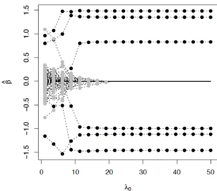
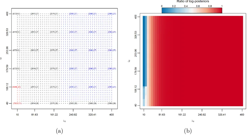
Figure 3a shows the trajectory of the number of non-zero βj,k’s and ωk,k0’s identified at a
subset of putative modes ˆΞs,t. Points corresponding to numerically unstable modes were
colored red and points corresponding to those ˆΞs,t for which the estimated supports of
B and Ω were identical to the estimated supports at ˆΞL,L, were colored blue. Figure 3a
immediately suggests a certain stabilization of our multivariate dynamic posterior
explo-ration. In addition to looking at
ˆ
B
0 and
ˆ Ω
0, we can look at the log-posterior density
of each ˆΞs,t computed with λ
0 = λ(0L), ξ0 = ξ0(L). Figure 3b plots a heat map of the ratio logπ(ˆΞs,t|Y)/π(ˆΞ0,0|Y)
logπ(ˆΞL,L|Y)/π(ˆΞ0,0|Y). It is interesting to note that this ratio appears to stabilize before the
(a) (b)
Figure 3: (a)Trajectory of (kBk0,kΩk0), (b) Trajectory of log(π(ˆΞ
s,t|Y)/π(ˆΞ0,0|Y)) log(π(ˆΞL,L|Y)/π(ˆΞ0,0|Y))
The apparent stabilization in Figure 3 allows us to focus on and report a single estimate
ˆ
ΞL,L, corresponding to the top-right point in Figure 3a, avoiding costly cross-validation.
Of course, this estimate is nearly indistinguishable from the estimates corresponding to the
other blue points in Figure 3a and we could just as easily report any one of them. On this
dataset, mSSL-DPE correctly identified 2360 out of the 2500 non-zeroβj,k’s with only 3 false
positives and correctly identified all 24 non-zeroωk,k0’s in the upper triangle of Ω,again with
only 3 false positive identifications. We should point out that there is no general guarantee
of stabilization for arbitrary ladders Iλ and Iξ. However, in all of the examples we have
tried, we found that stabilization occurred long beforeλ(0s)andξ0(t)reachedλ(0L)=ξ0(L)=n.
We should add that once the solutions stabilize, the algorithm runs quite quickly so the
excess computations are not at all burdensome.
2.3.1. Faster Dynamic Conditional Posterior Mode Exploration
mSSL-DPE can expend considerable computational effort identifying modal estimates ˆΞs,t
ˆ
ΞL,Lfrom mSSL-DPE is very promising, one might also consider streamlining the procedure
using the following procedure we term mSSL-DCPE for “Dynamic Conditional Posterior
Exploration.” First, we fix Ω =I and sequentially solve Equation (2.3) for each λ0 ∈ Iλ,
with warm-starts. This produces a sequence
n
ˆ
Bs,θˆs
o
of conditional posterior modes of
(B, θ)|Y,Ω = I. Then, holding (B, θ) = ( ˆB0L,θˆ0L) fixed, we run a modified version of our
dynamic posterior exploration to produce a sequence
n
ˆ Ωt,ηˆt
o
of conditional modes of
(Ω, η)|Y, B = ˆBL. We finally run our ECM algorithm from BˆL,θˆL,ΩˆL,ηˆL with λ
0 =
λL0 and ξ0 = ξ0L to arrive at an estimate of ΞL,L∗, which we denote ˜ΞL,L. We note that
the estimate returned by mSSL-DCPE, ˆΞL,L usually does not coincide with ˜ΞL,L. This is
because, generally speaking, when it comes time to estimate ΞL,L∗, DPE and
mSSL-DCPE launch the ECM algorithm from different starting points.
In sharp contrast mSSL-DPE, which visits several joint posterior modes before reaching an
estimate of posterior mode ΞL,L∗, mSSL-DCPE visits several conditional posterior modes
to reach another estimate of the same mode. On the same dataset from the previous
subsection, mSSL-DCPE correctly identified 2,169 of the 2,500 non-zero βj,k with 8 false
positives and all 24 non-zero ωk,k0’s but with 28 false positives. This was all accomplished
in just under 30 seconds, a considerable improvement over the two hour runtime of
mSSL-DPE on the same dataset. Despite the obvious improvement in runtime, mSSL-DCPE
terminated at a sub-optimal point whose log-posterior density was much smaller than the
solution found by mSSL-DPE. All of the false negative identifications in the support of
B made by both procedures corresponded to βj,k values which were relatively small in
magnitude. Interestingly, DPE was better able to detect smaller signals than
mSSL-DCPE. We will return to this point later in Section 2.3.2.
2.3.2. Simulations
We now assess the performance of mSSL-DPE and mSSL-DCPE on data simulated from
two models, one low-dimensional with n= 100, p= 50 andq = 25 and the other somewhat
according to a Np(0p,ΣX) distribution where ΣX =
0.7|j−j0|
p
j,j0=1.We construct matrix
B0 with pq/5 randomly placed non-zero entires independently drawn uniformly from the
interval [−2,2]. We then set Ω−01 =
ρ|k−k0|
q
k,k0=1 for ρ ∈ {0,0.5,0.7,0.9}. When ρ 6= 0,
the resulting Ω0 is tri-diagonal. Finally, we generate data Y = XB0+E where the rows
of E are independently N 0q,Ω−01
. For this simulation, we set λ1 = 1, ξ1 = 0.01nand set
Iλ and Iξ to containL= 10 equally spaced values ranging from 1 tonand from 0.1nton,
respectively.
We simulated 50 datasets according to each model, each time keepingB0 and Ω0 fixed but
drawing a new matrix of errors E. To assess the support recovery and estimation
per-formance, we tracked the following quantities: SEN (sensitivity), SPE (specificity), PREC
(precision), ACC (accuracy), MCC (Matthew’s Correlation Coefficient), MSE (mean square
error in estimatingB0), FROB (squared Frobenius error in estimating Ω0), and TIME
(ex-ecution time in seconds). If we let TP, TN, FP, and FN denote the total number of true
positive, true negative, false positive, and false negative identifications made in the support
recovery, these quantities are defined as:
SEN = TP
TP + FN PREC =
TP TP + FP
SPE = TN
TN + FP ACC =
TP + TN TP + TN + FP + FN
and
MCC = p TP×TN−FP×FN
(TP + FP) (TP + FN) (TN + FP) (TN + FN).
Table 1 – 4 reports the average performance, in both low- and high-dimesnional settings,
of mSSL-DPE, mSSL-DCPE,Rothman et al. (2010)’s MRCE procedure,Cai et al. (2013)’s
CAPME procedure, each with 5-fold cross validation, and the following two competitors:
Sep.L+G: We first estimate B by solving separate LASSO problems with 10-fold
using the GLASSO procedure of Friedman et al. (2008), also run with 10-fold
cross-validation
Sep.SSL + SSG: We first estimateB column-by-column, deployingRoˇckov´a and George
(2016)’s path-following SSL along the ladderIλ separately for each outcome. We then
run a modified version of our dynamic posterior exploration that holds B fixed and
only updates Ω and η with the ECM algorithm along the ladder Iξ. This is similar
to Sep.L+G but with adaptive spike-and-slab lasso penalties rather than fixed `1
penalties.
In the previous subsection, we took aθ = 1, bθ = pq, aη = 1 and bη = q. These
hyper-parameters placed quite a lot of prior probability on rather sparse B’s and Ω’s. Earlier
we observed that with such specification we achieved reasonably good support recovery of
the true sparse B and Ω.The extent to which our prior specification drove this recovered
sparsity is not immediately clear. Put another way, were our sparse estimates of B and
Ω truly “discovered” or were they “manufactured” by the prior concentrating on sparse
matrices? To investigate this possibility, we ran mSSL-DPE and mSSL-DCPE for the two
choices of (bθ, bη) = (1,1) and (bθ, bη) = (pq, q), keeping aθ = aη = 1. In Tables 1 – 4
mSSL-DPE(pq,q) and mSSL-DPE(1,1) correspond to the different settings of the
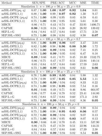
Table 1: Variable selection and estimation performance of several methods in low-dimensional settings. NaN indicates that the specified quantity was undefined, either be-cause no non-zero estimates were returned or bebe-cause there were truly no non-zero param-eters (Simulation 4). MSE has been re-scaled by a factor of 1000 and TIME is measured in seconds
Method SEN/SPE PRE/ACC MCC MSE TIME
Simulation 1: n= 100, p= 50, q= 25, ρ= 0.9
mSSL-DPE(pq, q) 0.87 /1.00 1.00/0.97 0.92 1.04 8.61 mSSL-DPE(1,1) 0.88 /1.00 0.99 /0.97 0.92 1.30 9.17 mSSL-DCPE (pq,q) 0.74 /1.00 0.99 / 0.95 0.83 6.59 0.41 mSSL-DCPE(1,1) 0.75 /1.00 0.98 / 0.95 0.83 5.61 0.30 MRCE 0.86 / 0.71 0.43 / 0.74 0.47 33.91 1406.71 CAPME 0.96/ 0.23 0.24 / 0.38 0.20 26.92 139.02 SEP.L+G 0.84 / 0.84 0.57 / 0.84 0.60 17.71 2.58 SEP.SSL+SSG 0.73 /1.00 0.98 / 0.94 0.82 8.98 0.07
Simulation 2: n= 100, p= 50, q= 25, ρ= 0.7
mSSL-DPE(pq,q) 0.81 /1.00 0.99/0.96 0.87 3.47 2.04 mSSL-DPE(1,1) 0.82 /1.00 0.98 /0.96 0.88 3.30 1.72 mSSL-DCPE(pq,q) 0.73 /1.00 0.99/ 0.94 0.82 7.41 0.25 mSSL-DCPE(1,1) 0.74 /1.00 0.99/ 0.95 0.83 6.47 0.18 MRCE 0.89/ 0.66 0.41 / 0.71 0.45 18.30 1532.75 CAPME 0.86 / 0.75 0.47 / 0.77 0.51 23.94 140.14 SEP.L+G 0.85 / 0.84 0.57 / 0.84 0.60 17.59 2.63 SEP.SSL+SSG 0.73 /1.00 0.99/ 0.94 0.82 8.61 0.06
Simulation 3: n= 100, p= 50, q= 25, ρ= 0.5
mSSL-DPE(pq,q) 0.76 /1.00 0.99/0.95 0.84 5.98 1.32 mSSL-DPE(1,1) 0.78 / 0.99 0.97 /0.95 0.85 5.53 1.11 mSSL-DCPE(pq,q) 0.73 /1.00 0.99/ 0.94 0.82 8.33 0.22 mSSL-DCPE(1,1) 0.74 /1.00 0.98 /0.95 0.83 7.54 0.16 MRCE 0.91/ 0.66 0.40 / 0.71 0.46 9.86 664.97 CAPME 0.86 / 0.77 0.48 / 0.78 0.52 23.41 144.80 SEP.L+G 0.85 / 0.84 0.57 / 0.84 0.60 171.3 2.92 SEP.SSL+SSG 0.73 /1.00 0.99/ 0.94 0.82 8.36 0.05
Simulation 4: n= 100, p= 50, q= 25, ρ= 0
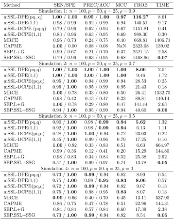
Table 2: Covariance selection and estimation performance of several methods in the low-dimensional setting. In these settings, theRimplementation of MRCE returned errors indi-cating over-fitting. NaN indicates that the specified quantity was undefined, either because no non-zero estimates were returned or because there were truly no non-zero parameters (Simulations 4). TIME is reported in seconds.
Method SEN/SPE PREC/ACC MCC FROB TIME
Simulation 1: n= 100, p= 50, q= 25, ρ= 0.9
mSSL-DPE(pq, q) 1.00/ 1.00 0.95/1.00 0.97 116.27 8.61 mSSL-DPE(1,1) 0.98 / 0.99 0.92 / 0.99 0.94 140.51 9.17 mSSL-DCPE (pq,q) 0.79 / 0.96 0.62 / 0.94 0.67 1151.81 0.41 mSSL-DCPE(1,1) 0.83 / 0.96 0.63 / 0.95 0.69 988.30 0.30 MRCE 0.96 / 0.73 0.24 / 0.75 0.40 669.81 1406.71 CAPME 1.00/ 0.00 0.08 / 0.08 NaN 2323.08 139.02 SEP.L+G 0.99 / 0.67 0.21 / 0.70 0.37 2521.15 2.58 SEP.SSL+SSG 0.79 / 0.96 0.63 / 0.95 0.68 1468.96 0.07
Simulation 2: n= 100, p= 50, q= 25, ρ= 0.7
mSSL-DPE(pq,q) 1.00/ 1.00 1.00/1.00 1.00 8.66 2.04 mSSL-DPE(1,1) 1.00/ 1.00 1.00/1.00 1.00 9.46 1.72 mSSL-DCPE(pq,q) 0.95 /1.00 0.94 / 0.99 0.94 28.53 0.25 mSSL-DCPE(1,1) 0.96 /1.00 0.95 / 0.99 0.95 21.43 0.18 MRCE 1.00/ 0.78 0.33 / 0.80 0.50 26.41 1532.75 CAPME 0.98 / 0.42 0.13 / 0.47 0.23 89.81 140.14 SEP.L+G 1.00/ 0.78 0.29 / 0.80 0.47 141.14 2.63 SEP.SSL+SSG 0.94 /1.00 0.95 / 0.99 0.94 40.60 0.06
Simulation 3: n= 100, p= 50, q= 25, ρ= 0.5
mSSL-DPE(pq,q) 0.90 /1.00 0.98 /0.99 0.94 5.62 1.32 mSSL-DPE(1,1) 0.92 /1.00 0.98 /0.99 0.94 6.13 1.11 mSSL-DCPE(pq,q) 0.28 /1.00 1.00/ 0.94 0.72 23.03 0.22 mSSL-DCPE(1,1) 0.45 /1.00 0.99 / 0.96 0.79 17.25 0.16 MRCE 1.00/ 0.82 0.33 / 0.83 0.51 6.63 664.97 CAPME 0.99 / 0.36 0.12 / 0.41 0.20 15.29 144.80 SEP.L+G 0.98 / 0.83 0.34 / 0.84 0.52 25.38 2.92 SEP.SSL+SSG 0.57 /1.00 0.99 / 0.97 0.74 13.78 0.05
Simulation 4: n= 100, p= 50, q= 25, ρ= 0
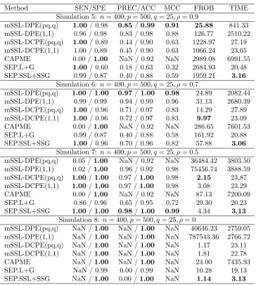
Table 3: Variable selection and estimation performance of several methods in the high-dimensional setting. In these settings, the R implementation of MRCE returned errors indicating over-fitting. TIME is reported in seconds.MSE has been re-scaled by a factor of 1000 and TIME is reported in seconds.
Method SEN/SPE PRE/ACC MCC MSE TIME
Simulation 5: n= 400, p= 500, q= 25, ρ= 0.9
mSSL-DPE(pq,q) 0.95/ 1.00 1.00/0.99 0.97 0.24 841.33 mSSL-DPE(1,1) 0.95/ 1.00 0.99 /0.99 0.96 0.58 2510.22 mSSL-DCPE(pq,q) 0.88 /1.00 0.99 / 0.97 0.92 1.40 27.19 mSSL-DCPE(1,1) 0.89 /1.00 0.99 / 0.98 0.92 1.25 23.65 CAPME 0.95/ 0.54 0.34 / 0.62 0.40 8.56 6991.55 SEP.L+G 0.92 / 0.76 0.48 / 0.79 0.56 10.32 20.48 SEP.SSL+SSG 0.88 /1.00 0.98 / 0.97 0.91 2.28 3.16
Simulation 6: n= 400, p= 500, q= 25, ρ= 0.7
mSSL-DPE(pq,q) 0.92/ 1.00 0.98 /0.98 0.94 0.86 2082.44 mSSL-DPE(1,1) 0.92/ 1.00 0.98 / 0.94 0.94 1.22 2680.39 mSSL-DCPE(pq,q) 0.88 / 1.00 0.99/ 0.97 0.97 1.63 27.89 mSSL-DCPE(1,1) 0.89 / 1.00 0.98 / 0.97 0.92 1.54 23.09 CAPME 0.67 / 0.84 0.53 / 0.81 0.48 110.13 7601.53 SEP.L+G 0.92/ 0.76 0.48 / 0.79 0.56 10.25 20.88 SEP.SSL+SSG 0.88 /1.00 0.98 / 0.97 0.91 2.23 3.06
Simulation 7: n= 400, p= 500, q= 25, ρ= 0.5
mSSL-DPE(pq,q) 0.91 / 0.60 0.38 / 0.66 0.42 34.23 3803.50 mSSL-DPE(1,1) 0.92/ 0.55 0.35 / 0.62 0.38 35.59 3888.59 mSSL-DCPE(pq,q) 0.88 /1.00 0.99/0.97 0.92 1.91 23.87 mSSL-DCPE(1,1) 0.89 / 0.99 0.98 /0.97 0.91 1.82 23.29 CAPME 0.65 / 0.86 0.54 / 0.82 0.48 116.42 7200.09 SEP.L+G 0.92/ 0.76 0.49 / 0.79 0.56 10.21 20.23 SEP.SSL+SSG 0.88 /1.00 0.98 /0.97 0.91 2.21 3.13
Simulation 8: n= 400, p= 500, q= 25, ρ= 0
Table 4: Covariance selection and estimation performance of several methods in the high-dimensional setting. In these settings, theRimplementation of MRCE returned errors indi-cating over-fitting. NaN indicates that the specified quantity was undefined, either because no non-zero estimates were returned or because there were truly no non-zero parameters (Simulation 8). TIME is reported in seconds.
Method SEN/SPE PREC/ACC MCC FROB TIME
Simulation 5: n= 400, p= 500, q= 25, ρ= 0.9
mSSL-DPE(pq,q) 1.00/ 0.98 0.85/0.99 0.91 25.88 841.33 mSSL-DPE(1,1) 0.96 / 0.98 0.83 / 0.98 0.88 126.77 2510.22 mSSL-DCPE(pq,q) 1.00/ 0.89 0.44 / 0.90 0.63 1228.97 27.19 mSSL-DCPE(1,1) 1.00 / 0.89 0.45 / 0.90 0.63 1066.24 23.65 CAPME 0.00 /1.00 NaN / 0.92 NaN 2989.08 6991.55 SEP.L+G 1.00/ 0.60 0.18 / 0.63 0.32 2684.93 20.48 SEP.SSL+SSG 0.99 / 0.87 0.40 / 0.88 0.59 1959.21 3.16
Simulation 6: n= 400, p= 500, q= 25, ρ= 0.7
mSSL-DPE(pq,q) 1.00/ 1.00 0.97/1.00 0.98 24.89 2082.44 mSSL-DPE(1,1) 0.99 / 0.99 0.94 / 0.99 0.96 31.13 2680.39 mSSL-DCPE(pq,q) 1.00/ 0.96 0.71 / 0.97 0.83 14.29 27.89 mSSL-DCPE(1,1) 1.00/ 0.96 0.72 / 0.97 0.83 9.97 23.09 CAPME 0.00 /1.00 NaN / 0.92 NaN 286.65 7601.53 SEP.L+G 0.99 / 0.87 0.40 / 0.88 0.58 161.92 20.88 SEP.SSL+SSG 1.00/ 0.96 0.70 / 0.96 0.82 57.88 3.06
Simulation 7: n= 400, p= 500, q= 25, ρ= 0.5
mSSL-DPE(pq,q) 0.05 /1.00 NaN / 0.92 NaN 36484.42 3803.50 mSSL-DPE(1,1) 0.02 /1.00 0.96 / 0.92 0.98 75456.74 3888.59 mSSL-DCPE(pq,q) 1.00/ 1.00 0.97 /1.00 0.98 2.15 23.87 mSSL-DCPE(1,1) 1.00/ 1.00 0.97 /1.00 0.98 3.08 23.29 CAPME 0.00 /1.00 NaN / 0.92 NaN 87.13 7200.09 SEP.L+G 0.86 / 0.96 0.65 / 0.95 0.72 29.30 20.23 SEP.SSL+SSG 1.00/ 1.00 0.98/1.00 0.99 4.34 3.13
Simulation 8: n= 400, p= 500, q= 25, ρ= 0
mSSL-DPE(pq,q) NaN /1.00 NaN / 1.00 NaN 40646.23 2759.05 mSSL-DPE(1,1) NaN /1.00 NaN / 1.00 NaN 787543.36 2766.72 mSSL-DCPE(pq,q) NaN /1.00 NaN / 1.00 NaN 1.17 23.11 mSSL-DCPE(1,1) NaN /1.00 NaN / 1.00 NaN 1.81 22.78 CAPME NaN /1.00 NaN / 1.00 NaN 24.00 7435.93 SEP.L+G NaN / 0.99 0.00 / 0.99 NaN 10.28 19.13 SEP.SSL+SSG NaN /1.00 0.00 /1.00 NaN 1.14 3.13
In both the high- and low-dimensional settings, we see immediately that the regularization
methods utilizing cross-validation (MRCE, CAPME, and SEP.L+G) are characterized by
high sensitivity, moderate specificity, and low precision in recovering the support of both
B and Ω.The fact that the precisions of these three methods are less than 0.5 highlights
rather unattractive feature from a practitioner’s standpoint! This is not entirely
surpris-ing, as cross-validation has a well-known tendency to over-select. In stark contrast are
mSSL-DPE, mSSL-DCPE, and SEP.SSL+SSG, which all utilized adaptive spike-and-slab
penalties. These methods are all characterized by somewhat lower sensitivity than their
cross-validated counterparts but with vastly improved specificity and precision,
perform-ing exactly as anticipated byRoˇckov´a and George (2016)’s simulations from the univariate
setting. In a certain sense, the regularization competitors cast a very wide net in order to
capture most of the non-zero parameters, while our methods are much more discerning. So
while the latter methods may not capture as much of the true signal as the former, they do
not admit nearly as many false positives.
CAPME, SEP.L+G, and SEP.SSL+SSG all estimate B in a column-wise fashion and are
incapable of “borrowing strength” across outcomes. MRCE and mSSL-DPE are the only two
methods considered that explicitly leverage the residual correlation between outcomes from
the outset. As noted above, in the low-dimensional settings, MRCE tended to over-select
inB and Ω,leading to rather poor estimates of both matrices. Moreover, in Simulations 5
– 8, the standardRimplementation of MRCE returned errors indicating over-fitting during
the cross-validation. In all but Simulations 7 and 8, mSSL-DPE displayed far superior
estimation and support recovery performance than MRCE.
Recall that mSSL-DCPE proceeds by finding a conditional mode
ˆ
BL,θˆL
fixing Ω = I,
finding a conditional mode
ˆ ΩL,ηˆL
fixing B = ˆBL, and then refining these two
condi-tional modes to a single joint mode. It is only in this last refining step that mSSL-DCPE
introduces the correlation between residuals to its estimation of B. As it turns out, this
final refinement did little to change the estimated support of B, so the nearly identical
performance of SEP.SSL+SSG and mSSL-DCPE is not that surprising. Further, the only
practical difference between the two procedures is the adaptivity of the penalties on βj,k:
in SEP.SSL+SSG, the penalties separately adapt to the sparsity within each column of B