A rule-based ad hoc method for selecting a bandwidth in kernel home-range analyses

bandwidth in kernel home-range analyses

Kie

R E S E A R C H

Open Access

A rule-based

_{ad hoc}

method for selecting a

bandwidth in kernel home-range analyses

John G Kie

Abstract

Background:An important issue in conducting kernel home-range analyses is the choice of bandwidth or smoothing parameter. To examine the effects of this choice, telemetry data were collected at high sampling rates (843 to 5,069 locations) on 20 North American elk,Cervus elaphus,in northeastern Oregon, USA, during 2000, 2002, and 2003. The elk had their collars replaced annually, hence none were monitored for more than a single year. True home ranges were defined by buffering the actual paths of individuals. Fixed-kernel and adaptive-kernel estimates were then determined with reference bandwidths (href), least-squares cross-validation bandwidths (hlscv), and

rule-basedad hocbandwidths designed to prevent under-smoothing (had hoc). Both raw data and sub-sampled

sparse datasets (1, 2, 4, 6, 12, and 24 locations/elk/day) were used.

Results:With fixed-kernel and adaptive-kernel analyses, reference bandwidths were positively biased (including areas not part of an animal’s home range) but performed better (lower bias, closer match between estimated and true home ranges) with increasing sample size. Least-squares cross-validation bandwidths were positively biased with very small sample sizes, but quickly became negatively biased with increasing sample size, as home-range estimates broke up into disjoint polygons.Ad hocbandwidths outperformed reference and least-squares cross-validation bandwidths, exhibited only moderate positive bias, were relatively unaffected by sample size, and were characterized by lower Type I errors (falsely including areas not part of the true home range).Ad hocbandwidths also exhibited lower Type II errors (failure to include portions of the true home range) than did least-squares cross-validation bandwidths, although reference bandwidths resulted in lowest Type II error rates. Auto-correlation indices increased to about 150 to 200 locations per elk, and then stabilized. Bias of fixed-kernel analyses withad hoc bandwidths was not affected by auto-correlation, but did increase with irregularly shaped home ranges with high fractal dimensions.

Conclusions:The rule-basedad hocbandwidths, specifically designed to prevent fragmentation of estimated home ranges, outperformed bothhrefandhlscv, and gave the smallest value forhconsistent with a contiguous

home-range estimate. The protocol for choosing thead hocbandwidth was shown to be consistent and

repeatable.

Keywords:Adaptive kernel, Bandwidth,Cervus elaphus, Fixed kernel, Home range, North American elk, Smoothing parameter

Correspondence: [email protected]

Department of Biological Sciences, Idaho State University, 921 South 8th Avenue, Stop 8007, Pocatello ID 83209-8007, USA

Background

A basic principal in animal ecology is that species, popu-lations, and individuals have finite limits in use of space. Species and populations are delineated by geographical ranges, and individuals are described as having a home range. Burt’s definition of home range is widely used:

‘…that area traversed by the individual in its normal ac-tivities of food gathering, mating and caring for young’ [1]. Although plotting animal locations is straightfor-ward, and is subject primarily to measurement errors, estimating the size of the home range is often dependent on a number of assumptions, which are often either not tested or if they are tested, are often determined to be false [2].

Kernel techniques for estimating the density of a utilization distribution (UD) of a random sample of loca-tions for an individual animal were first proposed by Worton [3]. Kernel analyses are commonly used in stat-istical density estimation and have the advantage of be-ing non-parametric [4]. They are used not only with single variables, but in bivariate space as well, with the distributions of thexandycoordinates representing ani-mal locations [3].

Although Worton [3] used the terms ‘utilization dis-tribution’ and ‘home range’synonymously, a distinction can be made between the two concepts. Early attempts to quantify the home range of an animal involved draw-ing polygons around the outermost set of locations. Such techniques result in a contiguous polygon delineating the ‘area traversed by the individual’ [1], including cru-cial travel corridors in which an animal spends limited amounts of time, but these fail to portray the intensity of space use within the polygon [5]. Conversely, kernel techniques provide a UD, that is, a three-dimensional probability density map showing which portions of the total home range home are used most frequently [5]. Al-ternatively, the estimate of the UD can be sliced to re-veal a two-dimensional (2D) surface (for example, by taking a 95% volume contour), which is the equivalent of a traditional definition of a home range. Such 2D slices may not be contiguous but rather disjoint, being composed of multiple polygons that more accurately in-dicate intensity of space use [6]. To capture little-used but important areas such as travel corridors, the 2D slice may be constrained to a single, contiguous polygon [5].

The starting point in kernel analyses is to construct a bivariate kernel estimate of a probability density function around each data point (animal location). A standard normal distribution is often used, although kernels can take on other shapes such as triangular, rectangular, or parabolic [4]. The functional shape and width of the kernel is determined by the smoothing parameter or bandwidth, denoted byh. Once probability density func-tions are in place, a grid structure is placed over the

entire field, and volumes under the functions are summed over individual locations.

The choice of a smoothing parameter is a key decision in home-range analyses involving UDs, and the initial value is often obtained from the data themselves, al-though there is noa prioriway to choose the best value forh. Silverman [4] and Worton [3] suggested a method of constructing an optimum h for large sample sizes if the data were assumed to be normally distributed. Re-ferred to ashopt(and occasionally, anad hocchoice ofh) by Worton [3], it is optimal only if the assumption of bi-variate normality is met, and will be denoted here as the reference bandwidthhref. If animal locations are clumped rather than normally distributed,hrefwill over-smooth the data, and the estimate of home-range size will be posi-tively biased [3].

A different approach is to choose a bandwidth that minimizes the least-squares cross-validation score, hlscv [3,7]. In most instances,hlscvis less thanhref, and is often only a small proportion of the latter. Although mathem-atically appropriate [3], hlscvfrequently results in under-smoothing, and gives an estimate of the home range that consists of multiple polygons. In extreme instances, such an estimate will generate polygons around each small cluster of points, or even individual points.

A further smoothing issue is whether to use the same

h for all points (global bandwidth), resulting in a fixed-kernel analysis, or to allow h to vary as a function of local point densities (local bandwidths), yielding an adaptive-kernel analysis. The local-bandwidth approach allows for larger kernels (greater smoothing) associated with locations, often at the edge of the animal’s distribu-tion, where location-point densities are lower. This ap-proach assigns more uncertainty to sparsely distributed locations near the edge of the home range [3].

An assumption of both kernel analyses and parametric approaches is that data points are independent. How-ever, animal locations are collected sequentially, and the extent to which the assumption of independence is vio-lated is a function of sampling rate [8]. Sampling rates are rapidly increasing with newer telemetry technologies, such as those based on global positioning systems [9]. Little information is currently available on how auto-correlation interacts with estimation choices in kernel analyses to bias resulting estimates. Moreover, the ability to assess bias and hence performance of different kernel techniques is ultimately dependent on defining the true home range of an animal, an issue that has not received much attention.

by connecting the locations test the efficiency of kernel analyses using both global and local bandwidths based onhrefand hlscv, and to suggest and test a new approach to choosing a smoothing parameter or bandwidth when conducting kernel home-range analyses.

Results

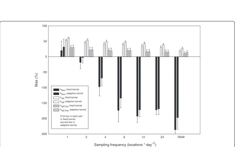
Estimates of bias in kernel analyses were affected by the individual animal (F19,700 = 6.93, P<0.0001), sampling frequency (F5,714 = 28.95, P<0.0001), and technique for choosing a bandwidth (F2,717 = 969.64, P<0.0001), but not by choice of fixed versus adaptive kernel (F1,718 = 0.44, P>0.10). Kernel analyses with a bandwidth that minimized the least-squares cross-validation score (hlscv) exhibited positive bias with a sampling frequency of one location per day, then a severely increasing negative bias with increasing sampling frequency (Figure 2, Figure 3). This negative bias was a result of the estimated home range breaking up into multiple polygons as sample size increased (Figure 3). The effect of using a global band-width (fixed kernel) versus a local bandband-width (adaptive kernel) with hlscvwas significant only at 6 (P = 0.0014) and 12 (P = 0.0021) locations per day. The proportion

hlscv/href decreased with increasing sampling frequency (X ± SD = 0.77 ± 0.31, 0.42 ± 0.18, 0.21 ± 0.08, 0.14 ± 0.04, 0.11 ± 0.006, 0.10 ± 0.0003 at 1, 2, 4, 6, 12, and 24 locations per elk per day, respectively, and 0.10 ± 0.0001 (raw data)).

Kernel analyses with the reference bandwidth (href) exhibited a consistent positive bias as a function of sam-pling frequency, although the bias declined somewhat with larger sample sizes (Figure 3). Bias using href was generally not affected by choice of fixed versus adaptive kernel, with a significant difference (P = 0.0347) seen only when using raw data (Figure 3). In a manner similar tohref,had hocresulted in a slight positive bias in the esti-mation of the size of home range, although the bias was more stable with respect to sampling frequency. Bias usinghad hocwas not affected as a function of fixed ver-sus adaptive kernel (all a priori combinations P>0.10) (Figure 3).

Figure 2Locations for elk 03.053 overlaid on true home range as defined in text.Also shown are home-range estimates using two kernel techniques (fixed and adaptive), three choices of smoothing parameter (hlscv, href, and had hoc), and four sampling frequencies (1, 4, and 12 location(s)

per day and the raw data).

Sampling frequency (locations * day-1)

1 2 4 6 12 24 RAW

Bias (%)

-250 -200 -150 -100 -50 0 50 100

hlscv fixed kernel

hlscv adaptive kernel

href fixed kernel

href adaptive kernel

had hoc fixed kernel had hoc adaptive kernel

First bar in each pair is fixed kernel, second bar is adaptive kernel

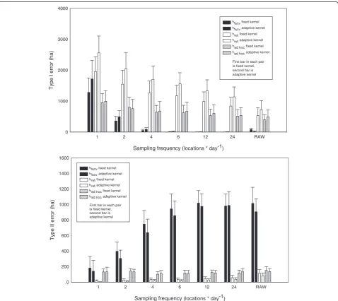
P<0.0001), but less so on the choice of fixed or adaptive-kernel approaches (F1,718 = 81.86, P<0.0001) (Figure 4). All techniques exhibited large Type I errors when a sam-pling frequency of 1 location per day was used, whereas the use of hlscv quickly resulted in a decrease in Type I errors with larger sample sizes, and effectively eliminated them at frequencies of four or more locations per day. This pattern was a result of the break-up of the estimate of home range into multiple polygons (Figure 2). Type I errors also decreased with sampling frequency when using href, but remained relatively constant when using had hoc(Figure 4).

Specifica prioricomparisons indicated that the choice of fixed versus adaptive kernel had a significant effect on Type I errors when using hlscv at a sampling frequency

of 1 location per day (P<0.0001),hrefat 1, 2, 4, 6, and 12 locations per day (P< 0.0001) and at 24 locations per day (P= 0.0006), and the raw data (P= 0.0226) (Figure 4). No significant differences (P> 0.10) between fixed and adap-tive kernels occurred at any sampling frequency when usinghad hoc(Figure 4).

Type II errors (failing to capture area in the estimate that was part of the animal’s home range) were affected by the individual animal (F19,700= 24.48,P<0.0001), sam-pling frequency (F5,714 = 92.57, P<0.0001), and method of choosing a bandwidth (F2,717 = 2,050.50, P<0.0001), but less by the choice of fixed or adaptive kernels (F1,718= 6.95, P = 0.0086) (Figure 4). When usinghlscv, significant differences existed between fixed and adap-tive kernels at two (P = 0.0335), four (P = 0.0121), and

Sampling frequency (locations * day-1)

1 2 4 6 12 24 RAW

Ty

pe II error (ha)

0 200 400 600 800 1000 1200 1400 1600

hlscv fixed kernel

hlscv adaptive kernel

hreffixed kernel

href adaptive kernel

had hoc fixed kernel

had hoc adaptive kernel

First bar in each pair is fixed kernel, second bar is adaptive kernel

Sampling frequency (locations * day-1)

1 2 4 6 12 24 RAW

Ty

pe I error (ha)

0 1000 2000 3000 4000

hlscvfixed kernel

hlscv adaptive kernel

href fixed kernel

href adaptive kernel

had hoc fixed kernel

had hoc adaptive kernel

First bar in each pair is fixed kernel, second bar is adaptive kernel

six (P= 0.0415) locations per day (Figure 4). All othera priori comparisons of fixed versus adaptive kernels within a sampling period or bandwidth selection tech-nique were not significant (allP>0.10) (Figure 4). Type II errors increased sharply withhlscvas the estimates of home range polygons became fragmented, but use of ei-ther href and had hoc resulted in Type II errors that remained relatively stable at less than 200 hectares as a function of sample size (Figure 4).

The elk locations used in this study were not inde-pendent, but exhibited serial correlation. The auto-correlation index of Swihart and Slade [8] increased with sampling frequency, reaching an asymptote of 2 to 3 at between 100 to 200 locations, corresponding to sam-pling frequencies of 4 to 6 locations per day (Figure 5a). Fixed-kernel analyses using had hoc as bandwidth indi-cated that bias did not differ as a function of auto-correlation index (Figure 5b), and hence, sampling frequency. Bias did increase with increasing fractal di-mension of the true home range (Figure 5c). As home ranges became more irregular in shape, the bias in home-range estimates increased.

Discussion and conclusions

Kernel analyses are widely used in estimating home ran-ges and UDs of animals, but they have some disadvan-tages. Choice of initial bandwidth largely determines the resulting estimates of home-range size (Figures 2, 3). A reference bandwidth (href) assumes bivariate normality, although samples of animal locations are frequently not normally distributed. Animals often use space in a clumped or multimodal manner, and href, in assuming a unimodal normal distribution, assigns high variance to the data when they are actually distributed more tightly around two or more modes. The result is over-smoothing of data, and an inflated estimate of home-range size. Conversely, a bandwidth that minimizes the least-squares cross-validation score (hlscv) often under-smoothes location data, and the resulting home-range estimate breaks up into disjointed polygons [5,6], resulting in negative bias in the estimate of home-range size (Figure 3) and large Type I errors (Figure 4).

Why should an estimate of the home range for an ani-mal be contiguous? One reason is philosophical; such a

Autocorrelation index

0.5 1.0 1.5 2.0 2.5 3.0 3.5 4.0

Bias (%)

-20 0 20 40 60

b

n locations

0 500 1000 4000 5000

Autocorrelation index

0.5 1.0 1.5 2.0 2.5 3.0 3.5 4.0

a

Fractal dimension

1.06 1.08 1.10 1.12 1.14 1.16

Bias (%)

-20 0 20 40 60

c

Figure 5Relationships between measured parameters. Relationships between(a)auto-correlation index [8] and number of locations,(b)between percentage bias and auto-correlation index, and(c)between percentage bias and fractal index of true home range for 20 elk sampled at 7 sampling frequencies (n= 140), derived from 95% fixed-kernel analyses usinghad hocchoice of

distribution matches Burt’s definition of home range as

‘that area traversed by the individual in its normal activ-ities of food gathering, mating, and caring for young [1]. Disjoint or separate core areas, such as those defined by a 60% kernel analysis, do not violate this definition, al-though an estimate of the entire home range that con-sists of multiple polygons does. For many purposes, such as estimating the intensity of spatial use of habitats [10], disjoint polygons are appropriate. Consequently, the terms ‘utilization distribution’and ‘home range’ are not synonymous, with only the former being a legitimate de-scription of disjoint spatial distributions. However, the biggest disadvantage to disjoint home-range polygons resulting from the use ofhlscvis that the degree of frag-mentation is highly dependent on sample size (Figure 2), which is an undesirable property when analyzing animal location data sampled at high frequencies with new and emerging telemetry technologies [9,11].

Given the disadvantages of kernel techniques, what available analytical options are essential to minimize bias and error? One issue is that as sampling frequency increases, so does serial auto-correlation. White and Garrott [2] argued that auto-correlation itself was not as much of an issue as was insuring that the sampling was evenly spread over the time period of interest. De Solla

et al. [12] also recommended maximizing the number of observations using constant time intervals, arguing that such a protocol increases the biological relevance of home-range estimation. In the current study, bias was not influenced by degree of auto-correlation when using

had hocchoice of bandwidth (Figure 5b). Type I and II er-rors associated with had hoc also appeared to be inde-pendent of sampling frequency (Figure 3). Given an appropriate choice of bandwidth such as had hoc, auto-correlation is not a concern. However, use of hlscv, is fraught with pitfalls associated with sampling frequency, auto-correlation, bias, and Type I and II errors. The issue is not whether an assumption of independent data has been violated, but rather how robust is a specific choice of bandwidth to such violations. This study indi-cates that kernel analyses using had hoc can be robust under these conditions, and supports previous recom-mendations [2,12].

Likewise, the shape of the kernel itself may not be a crucial issue. Wand and Jones [13] noted that that effi-ciency of various kernel shapes varied by less than 10%. Most computer programs currently use a standard nor-mal distribution for the kernel probability density func-tion [14]. However, other shapes are possible, including uniform or triangular kernels [4,13]. Some older pro-grams use a parabola-shaped Epanechnikov kernel to avoid having to evaluate the volume under the extended tails of a bivariate normal distribution [15]. It should be noted that computationally, it is not possible to conduct

a strict 100% volume analysis with a standard-normal kernel; the tails of the kernel must be truncated at some point by requesting a volume of less than 100%. In some computer programs, this modification may be done automatically, for example at 99.9%, in a manner not transparent to the user. Although not tested in this study, it has been suggested that choice of kernel shape is not of major concern [13].

The advantages and disadvantages of using global ver-sus local bandwidths in kernel home-range analyses has been the subject of debate, as has the choice of h [7]. Worton [3] favored a local bandwidth (adaptive kernel) using hlscv, but also suggested that a global bandwidth (fixed kernel) using href also produced valid estimates. Worton [16] later argued that although the choice of h

was very important, the choice of global versus local ap-plication of that bandwidth was less so. Seaman and Powell [17] and Seaman et al. [18] reported that global use of hlscv resulted in little bias in home-range esti-mates, but that local-bandwidth approaches overestima-ted areas of distribution, and thus should not be used. The results from the current study are consistent with Worton [16]; the choice between global versus local bandwidths is inconsequential in terms of bias (Figure 3), Type I, and Type II errors (Figure 4). Conversely, in this study the use ofhlscvresulted in rapidly increasing nega-tive bias and Type I errors in home-range estimates with increasing sample size (Figures 2, 4). Similar concerns have been raised by Hemsonet al. [19].

Different computer programs have limits on how small

hlscvcan be as a function of href. Home Range Extension (HRE) places a minimum value ofhlscvat 0.1025href[14], a floor unlikely to have a pronounced effect on the cal-culation of hlscv in this study. However, another com-monly used program (Animal Movement Extension, http://alaska.usgs.gov/science/biology/spatial/gistools/ index.php/, accessed 29 January 2013) will not allow a value forhlscvof less than 0.9662href, in effect implemen-ting an incorrect definition ofhlscv(= 0.9662href) in many analyses (A. Rodgers, personal communication).

The current study indicates that implementation of

are consistent and repeatable, and have been used in other studies [23,24].

With emerging telemetry techniques, large numbers of data on animal location can be collected at high sam-pling frequencies [9]. The technique of plotting the buffered path of an individual [25,26], similar to that performed in this study to define true home ranges, may provide a useful estimate of the total area used by an animal. However, further research into perceptual ranges of different species [27,28] will be required refine the distance by which animal paths should be buffered. Con-versely, for the foreseeable future, kernel approaches will remain useful for the analysis of spatial use by animals, not only for use with sparse datasets, but most import-antly for determining intensity of use within a home range.

Methods Study area

This study was conducted at the US Forest Service’s Starkey Experimental Forest and Range (hereafter re-ferred to as ‘Starkey’), located 35 km southwest of La Grande (45°13’N, 118°31’W) in the Blue Mountains of northeastern Oregon, USA (Figure 1). The forest is situ-ated between 1,122 and 1,500 meters in elevation, and supports a mosaic of coniferous forests, grasslands, and riparian areas that typify the summer range for elk in the Blue Mountains [29]. A network of narrow, irregular drainage channels in the project area creates a complex and varied topography [30,31].

Starkey consists of 10,125 hectares enclosed by a 2.4-m high fence that prevents immigration or emigra-tion of resident elk and other large herbivores [29]. The largest division within Starkey is a main study area if 7,762 hectares, from which data for this research were obtained (Figure 1). Details of the study area and facil-ities are available elsewhere [29,32-34].

Determining animal locations

As part of ongoing research at Starkey on North American elk, mule, and domestic cattle, an automated radio tele-metry system was developed based on rebroadcast long range navigation (LORAN)-C signals in the late 1980s to collect location data on these ungulates [29]. For the current study, data were collected each November during 2000, 2002, and 2003. Periods of data collection coincided with the ability, dictated by the needs of other studies, to reduce the total number of animals being monitored, and thereby increase the sampling frequencies of study ani-mals (Table 1). To avoid lack of independence in data resulting from individuals traveling together in herds, an association-matrix approach was used [35]. Each year, a random sub-sample of four locations per day was drawn for each radio-collared elk. A temporal threshold of 1 day

and a spatial threshold of 183 m were used. Deposition of fecal pellet groups by elk and mule deer in open grass-lands in a forest-grassland mosaic declined at more than 183 m away from forested edges [36]. Hence, 183 m was judged a reasonable approximation for the perception threshold of the North American elk [27]. Data from one animal in each pair that was located within 183 m of each other 50% or more of the time on any given day were eliminated, thereby arriving at a final sample size of 20 fe-male elk for the 3 years of this study (Table 1). No indivi-dual was monitored for more than 1 year.

Ethic approval

Protocols were approved by the Institutional Animal Use and Care Committee at Starkey Experimental Forest and Range [37].

The female elk in this study were (mean ± SD) 6.9 ± 2.85 years of age (range 3 to 14 years). Mean elapsed times between observations were 36.90 ± 5.22 minutes (n = 3 elk) in 2000, 8.67 ± 0.92 minutes (n = 9) in 2002, and 8.95 ± 0.87 minutes (n = 8) in 2003. Numbers of lo-cations per individual ranged from 843 to 1,089 in 2000, and from 3,615 to 5,069 in 2002 to 2003 (Table 1).

Finally, to test the performance of different techniques for estimating home-range size using sparse datasets, data were sub-sampled by choosing at random 1, 2, 4, 6, 12, and 24 locations per elk per day. Techniques for home-range estimation were then applied to each dataset of reduced sampling frequency in addition to raw data. Moreover, bivariate serial auto-correlation and cross-correlation between 2 points, but among 3 or more points in the raw and sparse datasets were estimated with a measure described by Swihart and Slade [8].

To test the accuracy of location data obtained from in-dividual elk, each year a radio collar was placed at a known location and its position monitored regularly, along with the study animals. Based on approximately 3,000 locations determined each year for the fixed col-lars, the estimated error (mean ± SD) was 35.3 ± 35.9 m, comparing favorably with a previous estimate of 52.8 ± 5.87 m (mean ± SE) [38].

Analyses of home ranges

home range was estimated to give a measure of the ir-regularity of its shape.

HRE [14] for ArcView (ESRI, Redlands, CA, USA) was used to estimate elk home ranges. The 95% volumetric kernel analyses [3] were calculated using a variety of techniques, including both a global bandwidth (fixed kernel) and local bandwidth (adaptive kernel), all with a default resolution (70 × 70 cell grid) option in HRE [14]. Three different methods were used in choosing an initial bandwidth. The first was to use the reference bandwidth,

href; the second was to use the bandwidth that mini-mized the cross-validation score,hlscv; and the third was based on anad hocapproach.

Silverman stated that‘a natural method for choosing a smoothing parameter is to plot out several curves and choose the estimate that is most in accordance with one’s prior ideas about the density’ [4]. In the current study, the goal was to delineate a single, contiguous polygon representing a complete home range as de-scribed by Burt [1]. Therefore, the reference bandwidth (href) was sequentially reduced in 0.10 increments (0.9href, 0.8href, 0.7href,…0.1href). This rule-basedhad hocwas the

smallest increment ofhrefthat: 1) resulted in a contiguous rather than disjoint 95% kernel home-range polygon, and 2) contained no lacuna within the home range. When se-quentially reducinghref, lacuna occasionally appeared that subsequently disappeared at successively smaller values of

href. However, Once an estimate of the home range frac-tured into two or more polygons, the process of searching forhad hocwas halted. In most instances,hlscv<had hoc< href, although had hoc < hlscv < href was considered. Con-versely, we did not allow had hoc to be greater than href when the estimate of the home range was fragmented at

href, but accepted the fragmented estimate instead. Note that the definition of had hoc used in the current study should not be confused with the discussion of href as an ad hoc choice by Worton [3]. This ad hoc choice of a bandwidth has previously been used to delineate home ranges in coyotes,Canis latrans[23], and in pronghorns,

Antilocapra americana[24].

Finally, the various estimates of elk home ranges were compared with what were previously defined as true home ranges. Differences in size between the estimates and the true home range (% bias) and Type I (area

Table 1 Location data collected for Rocky Mountain elk at Starkey Experimental Forest and Range, Oregon, USA

Animal ID Locations, n Elapsed time, minutesa True home range

X SD Size, hectares Fractal dimension

31 October to 24 November 2000 (25 days)

00.068 843 42.85 61.10 1,983 1.149

00.134 1,038 34.79 38.50 1,061 1.091

00.486 1,089 33.07 32.63 965 1.084

2 November to 3 December 2002 (32 days)

02.073 5,069 7.84 9.25 1,861 1.097

02.077 4,911 8.10 10.23 1,616 1.123

02.151 4,998 7.97 10.09 904 1.098

02.240 4,655 8.55 25.72 1,880 1.075

02.252 3,615 10.97 30.73 1,087 1.077

02.256 4,601 8.62 25.05 741 1.097

02.267 4,626 8.60 25.04 1,692 1.095

02.275 4,564 8.72 12.13 1,722 1.071

02.330 4,952 8.67 12.21 1,327 1.114

4 to 30 November 2003 (27 days)

03.053 4,119 9.72 12.82 1,348 1.077

03.132 4,155 9.64 48.50 1,893 1.073

03.135 4,913 8.19 8.61 3,083 1.076

03.200 4,321 9.27 11.79 1,741 1.111

03.216 4,677 8.60 14.96 1,828 1.113

03.274 5,003 8.04 8.88 1,330 1.067

03.307 5,054 7.95 8.65 1,369 1.057

03.344 3,942 10.19 13.05 1,874 1.079

a

included as part of the estimate, which was not part of the true home range) and Type II errors (area within the true home range, which was not included within the es-timate), were examined. For kernel analyses, statistical tests were conducted with a general linear model in SAS software (SAS Institute, Cary, NC, USA) [39] with main factors including individual animal (n= 20), initial bandwidth (n =2: global, local), bandwidth selection technique (n = 3: href, hlscv, had hoc), and sampling fre-quency (n = 6: 1, 2, 4, 6, 12, and 24 locations per day plus raw data), along with interactions between the main factors. Total sample size was thus 720 records (20 × 2 × 3 × 6). Bias was transformed with a square-root arc sin function to ensure additivity of treatment effects [40], and specific a priori comparisons were made with least-squares means [39]. The relationship between per-centage bias of the various home-range estimates as functions of degree of auto-correlation between among of individual elk and the fractal dimension of the true home range was examined.

Abbreviations

2D:Two-dimensional; LORAN: Long range navigation; HRE: Home Range Extension; UD: Utilization distribution.

Competing interests

The author has no competing interests.

Acknowledgements

I thank Alan A. Ager for assistance with preparing raw data files for ArcView GIS, and R. T. Bowyer, A.R. Rodgers, and J. K. Young for comments on previous versions of this manuscript.

Received: 14 February 2013 Accepted: 29 July 2013 Published: 2 September 2013

References

1. Burt WH:Territoriality and home range concepts as applied to mammals. J Mammal1943,24:346–352.

2. White GC, Garrott RA:Analysis of Wildlife Radio-Tracking Data.San Diego, California: Academic; 1990.

3. Worton BJ:Kernel methods for estimating the utilization distribution in home-range studies.Ecology1989,70:164–168.

4. Silverman BW:Density Estimation for Statistics and Data Analysis. Monographs on Statistics and Applied Probability.London: Chapman and Hall; 1986.

5. Kie JG, Matthiopoulos J, Fieberg J, Powell RA, Cagnacci F, Mitchell MS, Gaillard J-M, Moorcroft PR:The home-range concept: are traditional estimators still relevant with modern telemetry technology?Phil Trans Royal Soc B2010,365:2221–2231.

6. Powell RA:Animal home ranges and territories and home range estimators. InResearch Technologies in Animal Ecology–Controversies and Consequences.Edited by Boitani L, Fuller TK. New York: Columbia University Press; 2000:65–110.

7. Gitzen RA, Millspaugh JJ:Comparison of least-squares cross-validation bandwidth options for kernel home-range estimation.Wildl Soc Bull2003, 31:823–831.

8. Swihart RK, Slade NA:Influence of sampling interval on estimates of home-range size.J Wildl Manage1985,49:1019–1025.

9. Tomkiewicz SM, Fuller MR, Kie JG, Bates KK:Global positioning system and associated technologies in animal behaviour and ecological research. Phil Trans Royal Soc B2010,365:2163–2176.

10. Marzluff JM, Millspaugh JJ, Hurvitz P, Handcock MS:Relating resources to a probabilistic measure of space use: forest fragments and Steller’s jays. Ecology2004,85:1411–1427.

11. Rodgers AR:Recent telemetry technology.InRadio Tracking and Animal Populations.Edited by Millspaugh JJ, Marzluff JM. San Diego, California, USA: Academic; 2001:79–121.

12. De Solla SR, Bonduriansky R, Brooks RJ:Eliminating autocorrelation reduces biological relevance of home range estimates.J Animal Ecol 1999,68:221–234.

13. Wand MP, Jones MC:Kernel Smoothing. Monographs on Statistics and Applied Probability 60.London: Chapman and Hall; 1995.

14. Rodgers AR, Carr AP:HRE: the Home Range Extension for ArcView.Thunder Bay, Ontario: Centre for Northern Forest Ecosystem Research, Ontario Ministry of Natural Resources; 1998.

15. Kie JG, Baldwin JA, Evans CJ:CALHOME: a program for estimating animal home ranges.Wildl Soc Bull1996,24:342–344.

16. Worton BJ:Using Monte Carlo simulation to evaluate kernel-based home range estimators.J Wildl Manage1995,59:794–800.

17. Seaman DE, Powell RA:An evaluation of the accuracy of kernel density estimators for home range analysis.Ecology1996,77:2075_–2085. 18. Seaman DE, Millspaugh JJ, Kernohan BJ, Brundige GC, Raedeke KJ,

Gitzen RA:Effects of sample size on kernel home range estimates.J Wildl Manage1999,63:739–747.

19. Hemson G, Johnson P, South A, Kenward R, Ripley R, Macdonald D:Are kernels the mustard? Data from global positioning system (GPS) collars suggests problems for kernel homerange analyses with least-squares cross-validation.J Animal Ecol2005,74:455–463.

20. Kie JG, Boroski BB:Cattle distribution, habitats, and diets in the Sierra Nevada of California.J Range Manage1996,49:482–488.

21. Kie JG, Bowyer RT, Boroski BB, Nicholson MC, Loft ER:Landscape heterogeneity at differing scales: effects on spatial distribution of mule deer.Ecology2002,83:530–544.

22. Bertrand MR, DeNicola AJ, Beissinger SR, Swihart RK:Effects of parturition on home ranges and social affiliations of female white-tailed deer. J Wildl Manage1996,60:899–909.

23. Berger KM, Gese EM:Does interference competition with wolves limit the distribution and abundance of coyotes?J Animal Ecol2007,76:1075–1085. 24. Jacques CN, Jenks JA, Klaver RW:Seasonal movements and home-range

use by female pronghorns in sagebrush-steppe communities of western South Dakota.J Mammal2009,90:433–441.

25. Ostro LET, Young TP, Silver SC, Koontz FW:A geographic information system method for estimating home range size.J Wildl Manage1999, 63:748–755.

26. Pulliainen E:Use of the home range by pine martens (Martes martesL.). Acta Zool Fennica1984,171:271–274.

27. Mech SG, Zollner PA:Using body size to predict perceptual range.Oikos 2002,98:47_–52.

28. Zollner PA:Comparing the landscape level perceptual abilities of forest sciurids in fragmented agricultural landscapes.Landscape Ecol2000, 15:523_–533.

29. Rowland MM, Bryant LD, Johnson BK, Noyes JH, Wisdom MJ, Thomas JW: The Starkey project: history, facilities, and data collection methods for ungulate research.US Forest Serv1997. General Technical Report PNW-GTR -396.

30. Ager AA, Johnson BK, Kern JW, Kie JG:Daily and seasonal movements and habitat use by female Rocky Mountain elk and mule deer.J Mammal 2003,84:1076_–1088.

31. Kie JG, Ager AA, Bowyer RT:Landscape-level movements of North American elk (Cervus elaphus): effects of habitat patch structure and topography.Landscape Ecol2005,20:289_–300.

32. Rowland MM, Coe PK, Stussy RJ, Ager AA, Cimon NJ, Johnson BK, Wisdom MJ:The Starkey habitat database for ungulate research: construction, documentation, and use.US Forest Serv1998. General Technical Report PNW-GTR-430.

33. Stewart KM, Bowyer RT, Kie JG, Cimon NJ, Johnson BK:Temporospatial distributions of elk, mule deer, and cattle: resource partitioning and competitive displacement.J Mammal2002,83:229–244.

34. Stewart KM, Bowyer RT, Kie JG, Dick BL, Ben-David M:Niche partitioning among elk, mule deer, and cattle: do stable isotopes reflect dietary niche?Ecoscience2003,10:297_–302.

35. Weber KT, Burcham M, Marcum CL:Assessing independence of animal locations with association matrices.J Range Manage2001,54:21–24. 36. Reynolds HG:Use of a ponderosa pine forest in Arizona by deer, elk, and

37. Wisdom MJ, Cook JG, Rowland MM, Noyes JH:Protocols for care and handling of deer and elk at the Starkey Experimental Forest and Range. US Forest Serv1993. General Technical Report PNW-GTR-311.

38. Findholt SL, Johnson BK, Bryant LD, Thomas JW:Corrections for position bias of a LORAN-C radio-telemetry system using DGPS.Northwest Sci 1996,70:273–280.

39. SAS Institute:SAS/STAT User's Guide, version 8.Cary, North Carolina: SAS Institute, Inc.; 1999.

40. Gilbert N:Biometrical Interpretation.Oxford: Clarendon Press; 1973.

doi:10.1186/2050-3385-1-13

Cite this article as:Kie:A rule-basedad hocmethod for selecting a bandwidth in kernel home-range analyses.Animal Biotelemetry20131:13.

Submit your next manuscript to BioMed Central and take full advantage of:

• Convenient online submission • Thorough peer review

• No space constraints or color figure charges • Immediate publication on acceptance

• Inclusion in PubMed, CAS, Scopus and Google Scholar

• Research which is freely available for redistribution