ORIGINAL ARTICLE
Kazunari Miyauchi · Koji Murata
Strain-softening behavior of wood under tension perpendicular to the grain
Abstract Three softwood samples and one hardwood sample were tested under a tension load applied along the radial direction using small clear specimens and the local tension strain was measured using the digital image correla-tion method. We successfully obtained a stress–strain curve with a strain-softening branch by calculating the stress using the strain distributions in the vicinity where the specimen ruptured. The continuous digital imaging of the specimen proved to be very effective for measuring the strain in quasi-brittle materials such as wood under tension. The nonlinearity of the stress–strain curve was quantifi ed using two parameters representing the deviation from linear elas-ticity, and the formula of the stress–strain curve was deduced from the interrelation between these parameters. This formula is expressed quite simply by using the modulus of elasticity along the radial direction and another constant that is unique to the material.
Key words Strain softening · Tension · Digital image cor-relation · Nonlinearity · Perpendicular to grain
Introduction
Recently, it has been widely recognized that linear elastic theory is not applicable to heterogeneous and quasi-brittle materials such as concrete, ceramics, and wood,1–3
and that a nonlinear stress–strain curve is required to predict the extent of damage or ultimate fracture. Several studies have investigated the nonlinear stress–strain relationship in the shearing of wood. Okusa4
and Yoshihara and Ohta5,6
con-K. Miyauchi (*) · K. Murata
Division of Forest and Biomaterials Science, Graduate School of Agriculture, Kyoto University, Kitashirakawa Oiwake-cho, Sakyo-ku, Kyoto 606-8502, Japan
Tel. +81-75-753-6236; Fax +81-75-753-6300 e-mail: [email protected]
Part of this article was presented at the 56th Annual Meeting of the Japan Wood Research Society, Akita, Japan, August 2006
ducted torsion tests on rectangular cross sections of wooden bars and theoretically examined the shear stress–shear strain relationship in the plastic region. On the other hand, Ukyo and Masuda7
conducted shear block tests and suc-ceeded in experimentally obtaining the true shear stress– shear strain curves with a strain-softening branch after the peak stress by calculating the shear stress distribution in the shear plane using the shear strain distribution in it.
Although wood under tension that is applied perpen-dicular to the grain is macroscopically brittle, it is also con-sidered to exhibit a strain-softening behavior. The basis for this conjecture can be attributed to the microscopic fracture and toughening mechanism – microcracking and crack bridging1,8
– in the vicinity where a specimen will ultimately rupture. However, such a stress–strain curve with a strain-softening branch has never been obtained experimentally for wood under transverse tension; this is because it is diffi cult to forecast where a specimen would rupture and measure the strain in that location. Therefore, we hypothe-sized that it might be possible to reveal the mechanical behavior in the vicinity of a rupture if the deformation of the tension test specimen was continuously recorded using a digital video camera and a digital image-analysis tech-nique was applied to measure the strain.
A formula for describing the nonlinear stress–strain rela-tionship is required to precisely simulate the behavior of materials or structural members using numerical analysis, for example, the nonlinear fi nite element method. In addi-tion, the peak stress can be regarded as the true strength when the stress–strain curve has a softening branch. Typi-cally, the Ramberg–Osgood formula9 has been used for elastoplastic materials. However, this formula is not useful for predicting the peak stress because of the monotone increasing function of strain. To avoid this shortcoming, O’Halloran proposed a formula that can represent the entire stress–strain curve and remarkably predict the peak stress in wood under compression.9
However, it is diffi cult to describe the strain-softening behavior by using this formula.
In this article, we report stress–strain curves with a soft-ening branch in wood subjected to a radial tensile load and
present a formula describing these curves. We have con-ceived a method to obtain a formula for the stress–strain curve with a softening branch in terms of the quantifi cation of the nonlinearity of this curve. For quasi-brittle materials such as concrete and ceramics, the degree of brittleness or the nonlinearity of load–displacement or stress–strain curves has been estimated using Hillerborg’s characteristic length or the parameters derived from it.10
Such parameters have also been applied to wood.11
These parameters are advantageous because they can be easily calculated from the load–displacement or stress–strain curve; however, the shape of the curve cannot be identifi ed by using only one parameter because its value might be similar for different curves. Therefore, in order to overcome this disadvantage, we expressed the nonlinearity of the stress–strain curve using two parameters.
Experimental
Specimen geometry and materials
The shape and dimensions of the tension test specimen were determined in conformance with JIS Z2101. The cross section of the specimen is dumbbell shaped, that is, narrow in the middle like a dumbbell. The details of the specimen geometry are shown in Fig. 1.
JIS Z2101 prescribes three specimen systems: the direc-tion of the tensile load and annual rings must form angles of 0° (T-system), 45° (TR-system), and 90° (R-system), where “T” and “R” indicate the tangential and radial direc-tions, respectively. In this study, the strain was measured over a small area. Thus, the variance of mechanical proper-ties such as the moduli of elasticity in the plane vertical to the loading axis was small for the R-system because this plane was located either in earlywood or latewood. This tendency simplifi es the analysis. However, for T- and TR-systems, the plane vertical to the loading axis had stripes of earlywood and latewood; therefore, the variance of mechan-ical properties in this plane was quite large. Therefore, in this study, the R-system was adopted.
Three softwood samples – spruce (Picea sp.), Douglas fi r (Pseudotsuga menziesii), and hinoki cypress
(Chamaecyp-aris obtusa) – and one ring-porous hardwood sample –
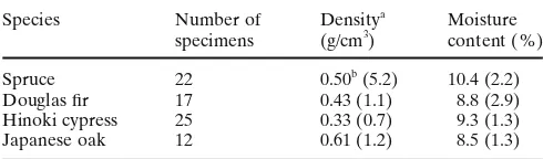
Japanese oak (Quercus cuspidata) – were chosen as specimens. After the specimens were cut, they were condi-tioned in a climate chamber at a temperature of 20°C and 60% relative humidity for several months. The oven-dry density and moisture content of all the specimens are listed in Table 1.
The digital image correlation method (DIC) was used to measure the deformation and calculate the strain in each specimen. The DIC program used in this study was coded by us and it had an accuracy of ±500 microstrains in the standard deviation.12
The DIC method facilitates the calcu-lation of the displacement vectors of any pixel point in a digital image by means of brightness pattern matching between images, and it requires random patterns of ness in the images. However, a wood surface has few bright-ness patterns, and hence the application of DIC to wood is diffi cult. Consequently, a random dot pattern was gener-ated on the specimen surface by spraying it with black or white water-soluble paint using an airbrush.
Testing method
The jigs holding each end of the tension test specimens to transmit the tensile load were mounted onto a hydraulic servoactuator (Instron; Model 8500) with a static load cell and on the stage of the testing machine. The tensile load was applied under displacement control and recorded at intervals of 1/3 s. The velocity of the crosshead of the testing machine was 0.7 mm/min for spruce and Japanese oak, 0.8 mm/min for Douglas fi r, and 1 mm/min for hinoki cypress. These loading conditions were determined such that rupture would occur in approximately 5 min.
In the tension test, the deformation of the specimen was continuously recorded using two digital video cameras (Sony; XCD-SX910). They were set equidistant from the specimen surfaces in order to acquire the images of the middle portion of the cross and radial sections of the speci-men (approximately 30 mm along the radial direction). The frame size of the monochrome digital images was 1024 × 768 pixels, and the longer side of the frame coincided with the radial direction of the specimen. Thus, the resolution of the images was approximately 0.03 mm/pixel.
The digital image-capture system (Library; Digital Capture) stores the digital data of the images in a personal computer’s temporary memory. Thus, the number of images that can be acquired is determined by the memory capacity of the personal computer and the size of each image. A
Cross section Radial section
10
20
20
(unit: mm) R65
35 25 30 25 35
Fig. 1. Japanese Industrial Standard (JIS) tension test specimen
Table 1. Properties of specimens
Species Number of Densitya Moisture specimens (g/cm3) content (%) Spruce 22 0.50b (5.2) 10.4 (2.2) Douglas fi r 17 0.43 (1.1) 8.8 (2.9) Hinoki cypress 25 0.33 (0.7) 9.3 (1.3) Japanese oak 12 0.61 (1.2) 8.5 (1.3)
a Oven-dry density
Windows XP system can store 2 gigabytes of data in temporary memory and the size of each image would be approximately 8 kilobytes; thus, a little more than 1000 images could be stored in each camera. Because the images were captured at intervals of 1/3 s, the deformation of the specimen could be recorded for 6 min.
Strain measurement using DIC
As shown in Fig. 2, the tensile load along the radial direc-tion caused the rupture of the specimen at the earlywood in an annual ring, which is the weakest layer in the speci-men. Japanese oak, which is a ring-porous wood, ruptured at a pore zone. Therefore, we hypothesized that the largest radial tensile strain could occur in this weakest layer and that we would be able to obtain the stress–strain curve with a strain-softening branch after the peak stress by investigat-ing the deformation behavior in this layer.
The tensile strain along the radial direction was calcu-lated using DIC. In the reference digital image, in which no deformation was observed before loading, a DIC analysis fi eld consisting of aligned elements was established at the region where the rupture would occur (Fig. 3). The number of elements was approximately 55 and 110 for the cross-section and radial-cross-section images, respectively. The strain in an element was calculated by measuring the displacement vectors of the four nodes that constitute the element.
If all the images had been used for DIC, the analysis would have required a large amount of time because approximately 800 images were obtained from each camera during a single tension test. Thus, 1 image captured just before the occurrence of rupture and 39 images captured at regular intervals under the applied tensile load were selected.
Results and discussion
Redistribution of tensile load
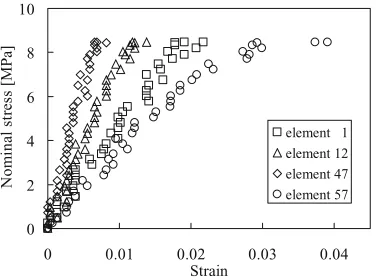
An example of the distribution of the radial tensile strain obtained using the DIC analysis is shown in Fig. 4. From this fi gure, it is evident that the strain was not uniformly distrib-uted in the earlywood of the specimen and that a consider-ably large tensile strain was concentrated in a narrow area. In addition, it is also assumed that the ultimate fracture originated from this area. The wide strain distribution can be ascribed to the fact that the tensile forces present in the elements for DIC were not equal. If this fact is neglected or if it is assumed that the tensile forces all over the elements are uniform, which implies that the nominal stress corre-sponds to the strain of each element, the stress–strain rela-tionships of all the elements are not found to be unique, as shown in Fig. 5. Thus, in order to obtain a unique
relation-2 mm
Fig. 2. Ruptured spruce specimen. Arrowheads indicate the annual ring boundaries
2 mm
Fig. 3. Digital image correlation (DIC) elements in the reference image
0 0.01 0.02 0.03 0.04
DIC element
St
rai
n
1760 N
1100 N 600 N
10 20 30 40 50
Fig. 4. Distributions of the radial tensile strain measured on the cross-sectional image of a spruce specimen
0 2 4 6 8 10
0 0.01 0.02 0.03 0.04 Strain
Nom
ina
l
st
res
s [MPa]
element 1 element 12 element 47 element 57
ship between the stress and strain, the tensile force in an element must be calculated by employing the redistribution of the tensile load following the straining of each element.7 Using this method, the stress can be calculated as follows:
σ ε
ε
i
i
i i
i N
P f
f A
= ⋅
⋅
=
∑
( ) { ( ) }
, 1
(1)
where s and e are the stress and strain along the radial direction, respectively; P, the tensile load; N, the number of elements or divisions in the transverse section; A, the area subjected to the tensile force; f(e), a weighting function; and index i denotes the ith element. When the sizes of the ele-ments are constant, Ai equals A/N, and Eq. 1 can be rewrit-ten as follows:
σ ε
ε σ
ε ε
i
i
i i
N
i P
A f
N f
f f
= ⋅ = ⋅
=
∑
( ) ( )
( ) ( ), 1
1
(2)
where s¯ is the nominal stress and f¯(e) is the average of
f(ei).
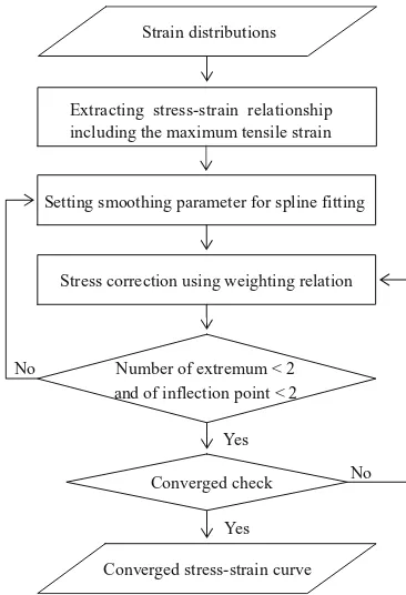
The concern emerging here is the determination of the appropriate weighting function to be used to distribute the tensile load. The relationship between the stress and strain can be used as a weighting function; therefore, if the stress– strain relationship is linear, we can simply substitute f(ei) with ei in Eq. 1. However, it is clear that this assumption is not applicable because of the nonlinear relationship between the stress and strain (Fig. 5). Hence, the tensile load must be redistributed using a nonlinear weighting function, which is not yet known. Therefore, we corrected a weighting func-tion iteratively and then obtained a single stress–strain curve. The procedure involved in this method is as follows. First, the stress–strain relationship of the element where the maximum tensile strain occurred was extracted and fi tted using a three-dimensional smoothing spline curve. Second, the weighting function f(e) in Eq. 1 was substituted with the smoothed curve and the stress was corrected. These two steps were iterated until all the stress–strain relationships converged onto a single curve. The fl ow for calculating the stress–strain curve is shown in Fig. 6. In this diagram, the fi fth step of the algorithm is required to exclude an impos-sible form of the stress–strain curve and to avoid the stress divergence during the iterative correction.
Strain-softening behavior
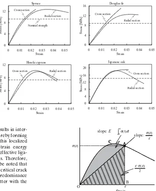
Examples of the stress–strain curves modifi ed by redistrib-uting the tensile load are shown in Fig. 7. Two solid curves in each graph were obtained from the strain distributions of the cross and radial sections of the same specimen, and the broken line represents the nominal tensile strength snom calculated by dividing the maximum tensile load by the initial area of the ruptured region. Because the tensile stress acting on the transverse section of the specimen was not uniform, the maximum strains measured on both sections were not necessarily equal. Of all the stress–strain curves,
47% exhibited strain-softening behavior and their peak stresses were attained at the following tensile strain ranges: Japanese oak, 0.021 ± 0.003; spruce, 0.024 ± 0.004; hinoki cypress, 0.030 ± 0.006; and Douglas fi r, 0.033.
The ratio of the maximum stress smax obtained from the stress–strain curve to the nominal tensile strength is listed in Table 2. The ratios for cross and radial sections were as follows: spruce, 1.43 ± 0.20 and 1.44 ± 0.18; Douglas fi r, 1.36
± 0.16 and 1.46 ± 0.22; hinoki cypress, 1.58 ± 0.24 and 1.27
± 0.11; and Japanese oak, 1.28 ± 0.16 and 1.25 ± 0.16. On the basis of the Douglas fi r example shown in Fig. 7, a lower maximum tensile strain exhibited the tendency to yield a more linear stress–strain curve and a larger maximum stress as compared with a higher maximum tensile strain yielding a stress–strain curve with a softening branch. This suggests that only when the strain softening appears, the maximum stress, which is equal to the peak stress in this case, can adequately approximate the true tensile strength.
The strain-softening behavior and fracture mechanism are closely related to each other when the tension is applied perpendicular to the grain. When an undamaged specimen is subjected to radial tensile stress, the specimen is sub-jected to strain, and microcracks begin to grow from the microscopic defects that inherently exist in cell walls and cell boundaries; this is followed by the occurrence of new microscopic defects. This damage is scattered throughout the system and uniformly decreases the capability of the system to transmit the tensile load or increases the compli-ance of the system. Consequently, the stress–strain curve deviates from linear elasticity and bends over. Moreover, the system remains stable as long as the elastic strain energy absorbed in the system increases, even if the stress begins
Extracting stress-strain relationship
Setting smoothing parameter for spline fitting Strain distributions
Stress correction using weighting relation
Number of extremum < 2 and of inflection point < 2
Converged check
Converged stress-strain curve Yes Yes
No No
including the maximum tensile strain
to decline. An increase in the tensile strain results in inter-cellular separation or intrainter-cellular fracture, thereby forming a localized critical crack surface.8
Although this localized fracture increases compliance, the elastic strain energy absorbed in the system decreases because the effective liga-ment that transmits the tensile load decreases. Therefore, the system becomes unstable. Here, it should be noted that the microcracking and the propagation of the critical crack are not exclusive but simultaneous, and predominance changes gradually from the former to the latter with the increase in strain.
Formula for stress–strain curves
We expressed the nonlinearity of the stress–strain curve using two parameters – u(e) and v(e) – in order to obtain a formula for the stress–strain curve with a softening branch. These parameters were defi ned as follows:
u
E v t dt
( ) ( ), ( ) ( ) ( )
,
ε σ ε
ε ε
ε σ ε σ
ε
=
⋅ =
⋅
∫
R 2
0
(3)
where ER is the modulus of elasticity along the radial direc-tion. As shown in Fig. 8, u(e) is the ratio of the stiffness at
e to the initial stiffness, and v(e) is the ratio of the elastic
strain energy density – area of OAB – to the strain energy density – area of OCAB – at e. The values of these param-eters range from zero to unity. If the materials exhibit linear elasticity, the values are unity; these values decrease with the degree of nonlinearity of the stress–strain curve. In order to characterize the nonlinearity of the stress–strain curve, we assumed, for convenience, that no plastic strain
Spruce
0 4 8 12
0 0.01 0.02 0.03 0.04 0.05
Strain
St
res
s [MPa]
Cross section
Nominal strength Radial section
Douglas fir
0 4 8 12 16
0 0.01 0.02 0.03 0.04 0.05
Strain
St
res
s [M
P
a]
Cross section
Radial section
Hinoki cypress
0 4 8 12
0 0.01 0.02 0.03 0.04 0.05
Strain
St
res
s [M
P
a]
Cross section Radial section
Japanese oak
0 4 8 12 16 20
0 0.01 0.02 0.03 0.04 0.05
Strain
St
res
s [MPa]
Cross section
Radial section
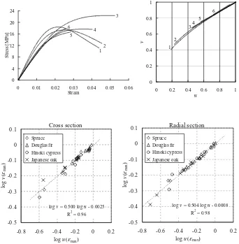
Fig. 7. Examples of stress–strain curves
Table 2. Ratio of maximum stress to nominal strength
Species Cross section Radial section
n smax (MPa) snom (MPa) smax/snom n smax (MPa) snom (MPa) smax/snom Spruce 16 (7) 12.4 ± 1.8 8.7 ± 0.9 1.43 ± 0.20 16 (7) 12.4 ± 1.2 8.7 ± 0.9 1.44 ± 0.18 Douglas fi r 4 (0) 12.3 ± 1.2 9.1 ± 0.2 1.36 ± 0.16 4 (1) 13.2 ± 1.7 9.1 ± 0.2 1.46 ± 0.22 Hinoki cypress 7 (2) 11.8 ± 2.0 7.5 ± 0.1 1.58 ± 0.24 7 (3) 9.5 ± 0.9 7.5 ± 0.1 1.27 ± 0.11 Japanese oak 9 (6) 16.8 ± 2.1 12.9 ± 1.1 1.28 ± 0.16 10 (8) 16.1 ± 2.2 12.9 ± 1.1 1.25 ± 0.16
n, Number of stress–strain curves and numbers in parentheses indicate those exhibiting strain-softening behavior; smax, maximum stress; snom,
nominal strength
A
B
C A
C
Strain
s(e)
e
O
A C
2 )
(e
s e·
slope: E
slope:
e e s()
∫
edt t s 0 ()
Fig. 8. Schematic diagram of nonlinearity of a stress–strain curve. The reciprocal of E is the initial compliance of a material and that of s(e)/e
was present. Nevertheless, this assumption is appropriate because, as mentioned in the previous section, the main cause of the nonlinearity in the stress–strain relationship is the decrease in the load transmission capability by the accumulation of microscopic fracture and the propagation of the critical crack; moreover, the undamaged region shows elastic behavior.
Some stress–strain curves with various nonlinearities and the corresponding u-v curves are shown in Fig. 9. The u-v curves converge on the same curvature despite the varying shapes of the stress–strain curves. This indicates that the fracture process is common to all the specimens and that all tensile stress–strain curves can be expressed by using a single formula.
In order to obtain the formula, the relationship between
u and v was investigated. u and v at the maximum strain emax were calculated as the representative values for all the stress–strain curves. As shown in Fig. 10, the u-v relationship was linear under a double logarithm and the gradient was 0.5, independent of the wood species. Therefore, the rela-tionship between u and v could be expressed as an expo-nential function as follows:
v( )ε =u( ) .ε 0 5.
(4) The formula for the stress–strain curves when the tension is applied perpendicular to the grain can be obtained by
substituting Eq. 3 in Eq. 4 and then solving the resulting equation. The stress–strain curve is expressed quite simply as follows:
σ ε ε
ε ε
( )= ⋅ ,
+
ER
inflect 1
2 2 (5)
where einfl ect is an integration constant and corresponds to the strain at the infl ection point of the stress–strain curve. In Eq. 5, the numerator represents linear elasticity and the denominator represents nonlinearity or the rate of increase in compliance, and it has a more signifi cant effect on the stress with a change in the strain. In addition, the estimation of the true tensile strength along the radial direction, sstrength, is expressed as follows:
σstrength= R⋅εinflect 3 3
16 E . (6)
The elastic strain energy density absorbed in the system, which corresponds to the area of OAB in Fig. 8, increases when e<einfl ect and decreases when einfl ect<e; that is, it is a maximum at e=einfl ect, because no plastic strain is assumed. Hence, the main fracture mechanism changes from micro-cracking to the propagation of the critical crack at e=einfl ect and the system becomes unstable. Therefore, einfl ect can be 0
4 8 12 16 20 24
0 0.01 0.02 0.03 0.04 0.05 0.06
Strain
St
re
ss
[M
P
a
]
1 2
3
4 5 6
0 0.2 0.4 0.6 0.8 1
0 0.2 0.4 0.6 0.8 1
u
v
1 2
4 5 6
3
Fig. 9. Stress–strain and u-v relationships of Japanese oak
log v = 0.504 log u - 0.0008
R2 = 0.98
-0.5 -0.4 -0.3 -0.2 -0.1 0 0.1
-0.8 -0.6 -0.4 -0.2 0 0.2 log u(emax)
log
v
(
emax
)
Spruce Douglas fir Hinoki cypress
Japanese oak
log v = 0.500 log u - 0.0025
R2 = 0.96
-0.5 -0.4 -0.3 -0.2 -0.1 0 0.1
-0.8 -0.6 -0.4 -0.2 0 0.2 log u(emax)
log
v
(
emax
)
Spruce Douglas fir Hinoki cypress Japanese oak
Cross section Radial section
regarded as a constant that is unique to each material char-acterizing the behavior of the deformation or fracture of wood.
Although Eq. 5 is based on the behavior of earlywood along the radial direction, this formula can be applied to latewood as well. We believe that further studies are required to confi rm this.
Conclusions
We conducted tension tests along the radial direction of wood and investigated the relationship between the stress and strain. Stress–strain curves with a strain-softening branch were obtained by calculating the stress using the strain distributions in the vicinity where the specimens rup-tured. The peak stresses were achieved at a tensile strain of 0.02–0.03. The nonlinearity of the stress–strain curve was quantifi ed using two parameters representing the deviation from linear elasticity. The formula for the stress–strain curve was deduced from the interrelation between these parame-ters. This formula is expressed quite simply using the modulus of elasticity along the radial direction and another constant unique to the material.
References
1. Vasic S, Smith I (2002) Bridging crack model for fracture of spruce. Eng Fract Mech 69:745–760
2. Stanzl-Tschegg SE, Tan DM, Tschegg EK (1995) New splitting method for wood fracture characterization. Wood Sci Technol 29:31–50
3. Tschegg EK, Frühmann K, Stanzl-Tschegg SE (2001) Damage and fracture mechanisms during mode I and mode III loading of wood. Holzforschung 55:525–533
4. Okusa K (1977) On the prismatical bar torsion of wood as elastic and plastic material with orthogonal anisotropy (in Japanese). Mokuzai Gakkaishi 23:217–227
5. Yoshihara H, Ohta M (1995) Shear stress–shear strain relationship of wood in the plastic region. Mokuzai Gakkaishi 41:529–536 6. Yoshihara H, Ohta M (1995) Determination of the shear stress–
shear strain relationship of wood by torsion tests. Mokuzai Gak-kaishi 41:988–993
7. Ukyo S, Masuda M (2004) Investigation of the true stress–strain relation in shear using the digital image correlation method (in Japanese). Mokuzai Gakkaishi 50:146–150
8. Smith I, Landis E, Gong M (2003) Fracture and fatigue in wood. Wiley, Chichester, pp 99–121
9. Bodig J, Jayne BA (1982) Mechanics of wood and wood compos-ites. Van Nostrand Reinhold, New York, pp 285–290
10. Harmuth H, Rieder K, Krobath M, Tschegg E (1996) Investigation of the nonlinear fracture behaviour of ordinary ceramic refractory materials. Mater Sci Eng A214:53–61
11. Reiterer A, Sinn G, Stanzl-Tschegg SE (2002) Fracture character-istics of different wood species under mode I loading perpendicular to the grain. Mater Sci Eng A332:29–36