Computational Methods for Analysis of Resting State Functional Connectivity and Their Application to Study of Aging

(1)

University of Pennsylvania

ScholarlyCommons

Publicly Accessible Penn Dissertations

1-1-2016

Computational Methods for Analysis of Resting

State Functional Connectivity and Their

Application to Study of Aging

Harini Eavani

University of Pennsylvania, [email protected]

Follow this and additional works at:http://repository.upenn.edu/edissertations

Part of theBiomedical Commons,Computer Sciences Commons, and theStatistics and Probability Commons

This paper is posted at ScholarlyCommons.http://repository.upenn.edu/edissertations/1695

Recommended Citation

Eavani, Harini, "Computational Methods for Analysis of Resting State Functional Connectivity and Their Application to Study of Aging" (2016).Publicly Accessible Penn Dissertations. 1695.

(2)

Computational Methods for Analysis of Resting State Functional

Connectivity and Their Application to Study of Aging

Abstract

The functional organization of the brain and its variability over the life-span can be studied using resting state functional MRI (rsfMRI). It can be used to define a "macro-connectome' describing functional interactions in the brain at the scale of major brain regions, facilitating the description of large-scale functional systems and their change over the lifespan. The connectome typically consists of thousands of links between hundreds of brain regions, making subsequent level analyses difficult. Furthermore, existing methods for group-level analyses are not equipped to identify heterogeneity in patient or otherwise affected populations.

In this thesis, we incorporated recent advances in sparse representations for modeling spatial patterns of functional connectivity. We show that the resulting Sparse Connectivity Patterns (SCPs) are reproducible and capture major directions of variance in the data. Each SCP is associated with a scalar value that is proportional to the average connectivity within all the regions of that SCP. Thus, the SCP framework provides an

interpretable basis for subsequent group-level analyses.

Traditional univariate approaches are limited in their ability to detect heterogeneity in diseased/aging

populations in a two-group comparison framework. To address this issue, we developed a Mixture-Of-Experts (MOE) method that combines unsupervised modeling of mixtures of distributions with supervised learning of classifiers, allowing discovery of multiple disease/aging phenotypes and the affected individuals associated with each pattern.

We applied our methods to the Baltimore Longitudinal Study of Aging (BLSA), to find multiple advanced aging phenotypes. We built normative trajectories of functional and structural brain aging, which were used to identify individuals who seem resilient to aging, as well as individuals who show advanced signs of aging. Using MOE, we discovered five distinct patterns of advanced aging. Combined with neuro-cognitive data, we were able to further characterize one group as consisting of individuals with early-stage dementia. Another group had focal hippocampal atrophy, yet had higher levels of connectivity and somewhat higher cognitive performance, suggesting these individuals were recruiting their cognitive reserve to compensate for structural losses. These results demonstrate the utility of the developed methods, and pave the way for a broader understanding of the complexity of brain aging.

Degree Type

Dissertation

Degree Name

Doctor of Philosophy (PhD)

Graduate Group

Bioengineering

First Advisor

(3)

Keywords

Aging, Functional Connectivity, Functional MRI, Heterogeneity, Machine Learning, Pattern Recognition

Subject Categories

(4)

COMPUTATIONAL METHODS FOR ANALYSIS OF RESTING STATE FUNCTIONAL CONNECTIVITY AND THEIR APPLICATION TO STUDY OF AGING

Harini Eavani

A DISSERTATION

in

Bioengineering

Presented to the Faculties of the University of Pennsylvania in Partial

Fulfillment of the Requirements for the Degree of Doctor of Philosophy

2016

Supervisor of Dissertation

Christos Davatzikos,

Professor of Radiology,

University of Pennsylvania

Graduate Group Chair

Jason A. Burdick,

Professor of Bioengineering,

University of Pennsylvania

DISSERTATION COMMITTEE

Paul Yushkevich, Professor of Radiology, University of Pennsylvania

Danielle Bassett, Assistant Professor of Bioengineering, University of Pennsylvania

Ted Satterthwaite, Assistant Professor of Psychiatry, University of Pennsylvania

Bruce Fischl, Professor of Radiology, Harvard Medical School

(5)

(6)

Acknowledgements

I would like to thank my advisor, Christos, for his guidance and support during

my tenure as a graduate student. I appreciate his immense knowledge and insight

in a very broad range of topics, which are extremely valuable in the highly

inter-disciplinary field of computational neuroscience. He gave me considerable freedom

to think and work independently, which was crucial to the synthesis of novel ideas.

I have learned a great deal from his lucid writing style and presenting complex

research ideas to any audience. Most of all, he invests a lot of time and resources

in his prot´eg´es’ careers, and is genuinely interested in seeing them grow into good

scientists. This is a rare attribute that sets him apart from everyone else.

I would also like to offer my gratitude to my collaborators Ted Satterthwaite,

Lori Beason-Held and Susan Resnick whose help shaped large parts of this thesis.

My shared experiences with fellow graduate students Aoyan, Maria, Erdem and Ke

made my time in the lab memorable. I would also like to thank my colleagues

Nicolas, Aris, Spyros, Mohamed, Michael, Guray, Jimit and Mark who have helped

me with my research projects time and time again.

Above all, this thesis is a testament to the unwavering support of my family and

their ability to put my needs above all else. I hope I can return the favor, at least to

(7)

ABSTRACT

COMPUTATIONAL METHODS FOR ANALYSIS OF RESTING STATE FUNCTIONAL

CONNECTIVITY AND THEIR APPLICATION TO STUDY OF AGING

Harini Eavani

Christos Davatzikos

The functional organization of the brain and its variability over the life-span can

be studied using resting state functional MRI (rsfMRI). It can be used to define a

“macro-connectome” describing functional interactions in the brain at the scale of

major brain regions, facilitating the description of large-scale functional systems

and their change over the lifespan. The connectome typically consists of thousands

of links between hundreds of brain regions, making subsequent group-level analyses

difficult. Furthermore, existing methods for group-level analyses are not equipped

to identify heterogeneity in patient or otherwise affected populations.

In this thesis, we incorporated recent advances in sparse representations for

modeling spatial patterns of functional connectivity. We show that the resulting

Sparse Connectivity Patterns (SCPs) are reproducible and capture major directions

of variance in the data. Each SCP is associated with a scalar value that is

propor-tional to the average connectivity within all the regions of that SCP. Thus, the SCP

framework provides an interpretable basis for subsequent group-level analyses.

Traditional univariate approaches are limited in their ability to detect

hetero-geneity in diseased/aging populations in a two-group comparison framework. To

address this issue, we developed a Mixture-Of-Experts (MOE) method that

com-bines unsupervised modeling of mixtures of distributions with supervised learning

of classifiers, allowing discovery of multiple disease/aging phenotypes and the

(8)

We applied our methods to the Baltimore Longitudinal Study of Aging (BLSA),

to find multiple advanced aging phenotypes. We built normative trajectories of

functional and structural brain aging, which were used to identify individuals who

seem resilient to aging, as well as individuals who show advanced signs of aging.

Using MOE, we discovered five distinct patterns of advanced aging. Combined with

neuro-cognitive data, we were able to further characterize one group as consisting

of individuals with early-stage dementia. Another group had focal hippocampal

atrophy, yet had higher levels of connectivity and somewhat higher cognitive

per-formance, suggesting these individuals were recruiting their cognitive reserve to

compensate for structural losses. These results demonstrate the utility of the

devel-oped methods, and pave the way for a broader understanding of the complexity of

(9)

List of Tables

2.1 Accuracy and AUC values for disriminative Sparse Learning, and

other methods . . . 48

3.1 Table comparing ten-fold cross-validation accuracy for MOE method

(14)

List of Figures

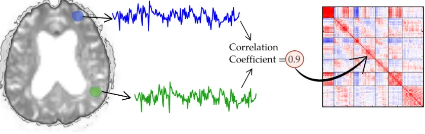
1.1 Figure illustrating computation of the functional connectome . . . . 2

1.2 Visualization of the functional connectome as a correlation matrix

(left), an abstract graph representation (middle) and mapped to

cor-responding regions in the brain (right) . . . 3

1.3 Left: Areal Graph nodes, as defined in Power et al. (2011). Right:

Common group-parcellation of GM regions obtained by running GraSP

(Honnorat et al., 2015) on BLSA data . . . 12

2.1 Schematic 1 illustrating our method. Each subject specific correlation

matrixΣnis approximated by a non-negative sum of sparse rank one

matricesbkbTk, or Sparse Connectivity Patterns (SCPs). . . 19

2.2 Schematic 2 illustrating our method. Each subject specific correlation

matrixΣnis approximated by a product of three factors - the

group-common matrixB, subject specific matrixCnandBT. . . 20

2.3 Visualization of SCPs. Opposing colors reflect anti-correlation

(15)

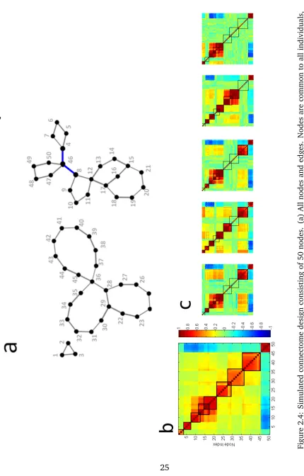
2.4 Simulated connectome design consisting of 50 nodes. (a) All nodes

and edges. Nodes are common to all individuals, different sets of

edges are inactive in different individuals. Edges in blue indicate

anti-correlation. (b) Average correlation matrix across all

individu-als. (c) Correlation matrices of five randomly chosen individuindividu-als. . . 25

2.5 Cross-validation results for simulated data: Plots of the mean square

error (Eqn. 2.3) vs. number of SCPs K (left), and sparsity level λ

(right). . . 26

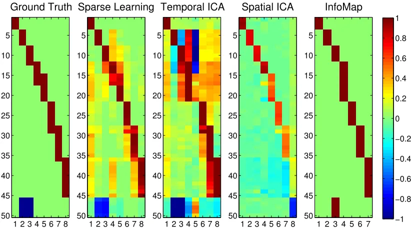
2.6 Performance on simulated data. The basis vectors identified by the

Sparse Learning approach, InfoMap, Spatial and Temporal ICA, shown

as node-weights (bk), compared against the ground-truth. . . 27

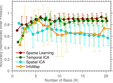
2.7 Performance on simulated data. Accuracy, measured using

normal-ized inner-product. . . 28

2.8 Individual-level coefficients estimated by Sparse Learning, projected

down to 2-D space, shown along with the ground truth. . . 29

2.9 Cross-validation results for PNC data: Plots of the mean square error

(Eqn. 2.3) vs. number of SCPs K (left), and sparsity levelλ (right). . 30

2.10 Ten SCPs computed in the Areal Graph node space. . . 31

2.11 Figure illustrating the heterogeneity of the data sample captured by

SCPs. The color indicates the extent to which each SCP is present in

a individual. . . 33

2.12 Reproducibility, data-fit, spatial overlap and temporal correlation

(16)

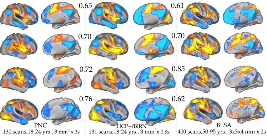
2.13 SCPs 1, 2, 5, and 9 computed from the PNC dataset(left), HCP+fBIRN

dataset (middle) and BLSA dataset (right) using Areal Graph nodes.

The inner product value (computed in the Areal Graph node space)

for each comparison is also shown. . . 38

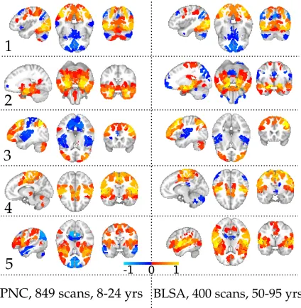
2.14 SCPs 1-5 generated from the PNC data (left) and BLSA data (right)

using GraSP parcels. . . 39

2.15 SCPs 6-10 generated from the PNC data (left) and BLSA data (right)

using GraSP parcels. Note that SCPs 9 and 10 do not match between

the two datasets. . . 40

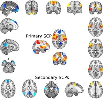
2.16 A primary SCP and some of its associated secondary SCPs computed

from the PNC dataset using GraSP parcels. . . 41

2.17 Split-sample error and reproducibility for secondary SCPs computed

from the PNC dataset. . . 42

2.18 SVM weight vector forl2-SVM (left) andl1-SVM (right) for

discrimi-nating children from young adults using the PNC dataset. . . 43

2.19 Schematic illustrating the discriminative Sparse Learning framework.

Panel to the left describes the SCP identification term, which

fac-torizes connectivity matrices Σn of each individual n into a set of

common SCPs B = [b1,b2, . . . ,bK] and its associated coefficients.

Panel to the right illustrates a linear SVM, which uses the total

ab-solute connectivity valuesdiag(BT_Σ

nB)of all SCPs as input features

(17)

2.20 Top two SCPs that contribute to classification, based on their

hyper-plane weight. Corresponding graphs (bottom) plot total connectivity

within SCP for each individual vs. individual age. Uni-variate

p-value scores comparing total connectivity between two groups are

also shown. . . 47

3.1 An illustration that shows heterogeneity in the affected group,

rela-tive to a reference group. Non-linear classifiers can implicitly model

non-linearity but estimating the boundary (dashed lines) in high

di-mensional spaces is difficult. Mixture-of-Experts can approximate the

non-linear curve with a piece-wise linear boundary (red and green

lines) and find subgroups associated with each line (red and green

points). . . 55

3.2 Four 2-D simulated cases used to evaluate the performance of the

method. Hyper-planes and sub-groups obtained using MOE are also

shown using a different color for each hyper-plane and associated

subgroup. . . 64

3.3 Variation in four performance measures for K = {1,2, . . . ,5}, for each of the four simulated cases. From top-left, clockwise: Accuracy,

Maximum inner-product, cluster separation and cluster

reproducibil-ity. Results from each case is plotted in a different color. . . 66

3.4 Variation in four performance measures forK = 3,C, λ={2−3_,₂−2_{, . . . ,}₂10_}_,

for Case 3. From top-left, clockwise: Accuracy, Maximum

inner-product, cluster separation and cluster reproducibility. . . 67

4.1 Age distribution for the subjects used in this study. For each age bin,

(18)

4.2 Scatter plot showing the relationship between age and motion

(mea-sured using MRD), which is statistically insignificant. The color

indi-cates the number of time-points that were removed during the

scrub-bing procedure. . . 74

4.3 (Above) Connectivity within the DM vs. DA SCP is significantly

de-creased with age. (Below) Connectivity within the medial temporal

areas is significantly increased with age . . . 75

4.4 Connectivity within the visual vs. DM areas (above) and motor areas

(below) is significantly decreased with age. . . 76

4.5 Eight secondary SCPs of the motor SCP, correlation between

corre-sponding coefficients and age, and associated p-value. . . 78

4.6 Brain Age Index of each individual plotted against their age. The

Mean Absolute Error (MAE) of prediction, as well as the correlation

coefficient between the BAI and age is provided. . . 79

4.7 Primary and associated secondary SCPs that were found to be

signif-icant after permutation testing. Although not all primary SCPs are

significant (faded images are not), they are shown for reference. . . . 81

4.8 Functional and structural Brain Age Indices (BAIs) plotted against

each individual’s age. Functional BAI was computed from SCP

coef-ficients and local functional coherence measures; structural BAI was

computed from average GM density values. The aging trajectories

(solid lines) show the expected brain age. The BAI Residual for each

individual in each modality can be computed by subtracting their

(19)

4.9 The DM vs. DA SCP alone shows significantly decreased connectivity

in the advanced agers relative to the resilient agers after correcting

for age. . . 82

4.10 Univariate differences in local functional coherence and GM density

between resilient and advanced agers. . . 83

4.11 Summary of significant differences in GM density, functional

coher-ence and connectivity for all five groups of advanced agers relative

to resilient agers. As before, changes to GM density and coherence

at the level of ROIs are shown using p-value maps overlaid on a

tem-plate image (first two columns on right). SCPs whose coefficients

were significantly different between groups are shown in the last

col-umn. The color overlay for SCPs indicates patterns of correlated (or

anti-correlated) regions. . . 85

4.12 Functional and structural BAI Residual (= Expected Brain age - BAI)

plotted in a two-dimensional grid. The group membership of each

individual is reflected in the color, resilient agers are shown as white

points. . . 87

4.13 Differences in cognitive performance between advanced group 1 and

resilient agers, for eight cognitive domains. Mean and 95%

confi-dence intervals of the difference estimates are shown as errorbars.

CVLT: California Verbal Learning Task. BVRT: Benton Visual

Reten-tion Test. CRDROT: Card RotaReten-tion Test. FLULET: Letter Fluency.

FLUCAT: Category Fluency. TRATS: Trail Making Test Part A. TRBTS:

Trail Making Test Part B. DSST: Digit Symbol Test. . . 88

(20)

5.2 Command-line interface of MOE . . . 100

A.1 SCPs computed without global signal regression, from the PNC dataset,

using the Areal Graph nodes. Only SCP 1 has a significant area of

negative correlation - the Dorsal Attention vs. Default mode

anti-correlation pattern. The other nine SCPs showed only positive

corre-lation. Of these, the familiar patterns were the sensori-motor (8, 9

(21)

Chapter 1 Introduction

1.1 Overview

Magnetic Resonance Imaging (MRI) provides a non-invasive, in-vivo method of

studying the human brain. In the clinic, these three-dimensional images of the brain

are used to identify gross abnormalities visible to the naked eye (lesions, tumours,

abscesses). In research applications, MRI is acquired from many research

partici-pants, in order to understand the subtle effects of development, aging or illness on

brain function and structure which cannot be observed by visual inspection.

Resting state functional MRI (rsfMRI) (Biswal et al., 1995; Raichle et al., 2001)

is acquired when the individual is at rest inside the scanner. It measures the blood

oxygenation level in different regions of the brain. Higher oxygen levels imply

higher neural activity, therefore fMRI is assumed to be a surrogate measure of brain

function. Multiple 3-D images are acquired, typically once every couple of seconds.

In this manner, we can obtain a time-series of varying blood oxygenation level at

ev-ery location in the brain. This “spontaneous” brain activity can be used to measure

(22)

Figure 1.1: Figure illustrating computation of the functional connectome

in the brain by quantifying the amount of synchrony between corresponding

activ-ity. This synchrony is popularly quantified by computing the Pearson correlation

coefficient between the corresponding time-series, as illustrated in Figure 1.1. In

this manner, one can build build a whole-brainfunctional connectomethat captures

a time-averaged picture of the functional interactions between all brain regions.

Figure 1.2 shows the various ways in which the functional connectome is visually

represented.

A growing number of projects (Satterthwaite et al., 2014; Van Essen et al., 2012;

Shock et al., 1984) are acquiring rsfMRI data for a large number of individuals with

the aim of investigating normal inter-subject variability and variation over the

lifes-pan. To keep pace with the scale of such projects, there is an urgent need to develop

novel methodology that can capture complex, whole-brain normative patterns of

age-related changes in a data-driven manner, while ensuring interpretability.

1.2 Aims of this thesis

The functional connectome of each individual is very high dimensional, however,

(23)

di-Figure 1.2: Visualization of the functional connectome as a correlation matrix (left), an abstract graph representation (middle) and mapped to corresponding regions in the brain (right)

mensionality reduction method that is based on functional connectivity data.

Exist-ing approaches for dimensionality reduction divide the brain into spatially smaller

patterns, varyingly referred to as components, sub-graphs or sub-networks. Some

of these existing approaches use the rsfMRI time-series as input, which is not ideal

for connectome data. Others assume spatial or temporal separation of the patterns,

which is not suited to describe functional systems in the brain. As we describe in

the following chapter, we exploited recent advances in the mathematics of sparse

modeling to develop a methodological framework that decomposes the complex

functional connectome into parsimoniousSparse Connectivity Patterns (SCPs). The

description of ourSparse Learningmethod and resulting SCPs is provided in Chapter

2 of this thesis.

In rsfMRI studies, univariate statistical approaches or multi-variate classification

methods are often employed to identify connections that can predict diseased state

of an individual or are strongly correlated with age. Such linear models inherently

assume that there is a single pattern of change that linearly scales with disease

severity or age in all individuals. However many of the conditions under study

(24)

composed of a variety of external symptoms and cognitive changes. In Chapter 3

of this thesis, we present aMixture-Of-Experts(MOE) method that explicitly models

and captures heterogeneous patterns of change in the affected group relative to a

reference group of controls.

Increased life expectancy has resulted in a growing proportion of older people

across the globe. This has led to a greater prevalence of aging related mental

ill-nesses. In order to better understand functional disruptions of such disorders, it

is crucial to gain insight into how the functional organization in the brain changes

during the normal aging process. Although, on average, cognitive abilities decrease

with age, some individuals age well, while other decline faster. Some of these

in-dividuals could be at a greater risk for developing clinical pathology later in life.

Therefore, in addition to understanding the effect of aging on function, it is

im-portant to identify these high-risk individuals, as well as potentially heterogeneous

patterns of aging. Towards this goal, we applied the methodological approaches

developed and tested in chapters 2 and 3 to rsfMRI data acquired as a part of the

Baltimore Longitudinal Study of Aging (BLSA). Multiple patterns of aging related

changes in connectivity are reported and discussed in Chapter 4.

These aims are summarized below:

1. Develop and test a method based on sparse representations for the

identifica-tion of resting-state connectivity networks

2. Develop and test a mixture of experts method for identification of

heterogene-ity in affected populations

3. Apply the developed methods to the BLSA dataset (normal adults of age 50-96

(25)

1.3 Significance

In order to make rsfMRI applicable to large heterogeneous populations, we require

automated data-driven analysis approaches that can capture the complexity of

func-tional connectivity patterns within the data. We summarize the significance of our

work vis-a-vis existing methods below, and discuss them in greater detail in

individ-ual chapters.

In Aim one, we proposed a sparsity-based dimensionality reduction algorithm

that is complementary to existing graph-based or time-series based methods. The

significance of this aim is described below:

1. Seed-based correlation approaches require prior knowledge of a stable seed

location and do not directly quantify inter-subject variability.

2. Graph-based approaches (Power et al., 2011) that identify networks based on

correlation strengths limit their analysis to strong positive correlations based

on an ad-hoc thresholding operation, ignoring thepositive-semi-definite

prop-erty of the correlation matrix. Negative and weak edges correlations could

be informative, especially if considered collectively as part of a distributed

pattern.

3. Graph-based methods are limited to identifying patterns in a group-averaged

manner (Power et al., 2011), thereby losing valuable information about

inter-individual variability.

4. Time-series based approaches, such as spatial (Beckmann et al., 2005) and

temporal ICA (Smith et al., 2012) have been successful in producing stable

and reproducible spatial components (especially spatial ICA). However (1)

(26)

not directly encode inter-individual variability in connectivity. This entails

novel methods that can directly explain the variance in connectivity data.

Aim two proposed a mixture of experts framework to address the drawbacks

of linear and non-linear supervised learning approaches, which are enumerated

below:

4. Multi-variate classification methods are needed to find subtle, distributed

pat-terns of aging related changes in the connectome. However, linear methods

assume a single pattern of aging or disease-related change, which is

unrealis-tic.

5. While kernel based methods can be used to model non-linear effects, the

pat-tern of change itself is not explicitly computed; kernel approaches do not

provide any information about the features that contribute to classification.

This motivates the need for developing methods that model heterogeneity in

the data explicitly.

As a part of the third aim, we applied the methods developed in Aims 1 and

2 to understand the effects of aging on functional connectivity. Previous studies

that investigated aging effects used traditional analysis approaches, whose major

limitations are described below:

6. Past studies investigating the effects of aging used mass-univariate approaches

to identify functional connections that significantly correlated with age.

How-ever, traditional analysis approaches make it difficult to gauge the extent and

severity of aging for each individual.

7. In prior studies of aging, small sample sizes limited researchers to assume

(27)

Using mass-univariate methods, an overall decrease in functional connectivity,

especially in the default mode and motor regions, has been found consistently.

However, a single pattern of change does not explain the wide variation in

cognitive abilities seen among the elderly. These studies did not stratify older

populations in terms of their patterns of change in brain structure and

func-tion.

1.4 Innovation

The major contributions of this thesis are summarized as follows:

1. The developed Sparse Learning method for the analysis of correlation matrices

does not require the removal of weak and negative correlation values. This

model represents the data as a combination of Sparse Connectivity Patterns,

while retaining the positive semi-definite nature of correlation matrices in the

representation. The P.S.D assumption constrains the degrees of freedom in

the model resulting in more stable, reliable networks.

2. We incorporated inter-individual variability in the strength of SCPs in our

modeling strategy. Such a model allocates a scalar value per pattern in each

individual that reflects the average connectivity of all the regions within that

particular pattern. This is a clear advancement over seed-based correlation

approaches, which do not consider individual level variations.

3. Sparse decompositions are being greatly favored in the signal processing

com-munity, as evidence of parsimony in nature as well as in the functioning of the

brain is abundant. We used spatial sparsity as the driving assumption for the

(28)

in sparse representations of covariance matrices (Sivalingam et al., 2011; Sra

and Cherian, 2011; Soufiani and Airoldi, 2012) in our modeling strategy.

4. The MOE framework for identification of heterogeneous patterns of change

explicitly models two crucial pieces of information that we would like to

dis-cover in the data - (1) multiple patterns that differentiate two groups and (2)

sub-groups of individuals associated with each pattern of change. The MOE

method has a complexity level that is in-between that of linear and non-linear

methods. Thus, it can capture more information than a linear method, while

at the same time is not as complex as the kernel-based method, and by design,

has better interpretability.

5. With data from the BLSA study, we used multi-variate methods to pool

infor-mation across all connections to predict each individual’s age. Using

multi-variate techniques, we identified those connections that highly contribute to

the prediction, similar to uni-variate techniques. More importantly, we built

aging trajectories of functional connectivity, similar to growth charts that are

used for children at the pediatrician’s office. Each individual is assigned a

Brain Aging Index (BAI), that measures the functional age of that individual.

We then identified a subset of individuals whose BAI is higher than their

ex-pected BAI. Theseadvanced agerscould be at a higher risk for developing signs

of dementia as they grow older.

6. We applied the MOE method to the advanced aging individuals (withresilient

agers as a reference) and identified sub-groups of advanced agers with

het-erogeneous patterns of functional and structural change. To the best of our

knowledge, we are the first to identify advanced aging patterns and

(29)

perspective.

1.5 rsfMRI data

1.5.1 Datasets

MRI data used in this thesis was acquired as a part of two major studies. Details of

the study participants and MR acquisition parameters are described in the following

section. Appendix A details the pre-processing pipeline that was used to prepare

rsfMRI data prior to generation of functional connectivity matrices.

1.5.1.1 Baltimore Longitudinal Study of Aging (BLSA)

The Baltimore Longitudinal Study on Aging (BLSA) (Shock et al., 1984) is the

longest running study on aging at the National Institute on Aging (NIA). It is a

lon-gitudinal study that acquires comprehensive cognitive assessments and MR brain

imaging measurements (and many others for physical health), from research

vol-unteers.

A subset of the data from this study was used for methodology testing in Chapters

2 and 3. A more extensive analysis of this data is described in Chapter 4.

Participants

As of February 1, 2015, BLSA had acquired 780 rsfMRI scans from 567 participants.

For this thesis, we considered only baseline (first visit) scans of participants selected

based on the following criteria: (1) participant was older than 50 years at time of

scan (2) had low head motion during the acquisition, measured using Mean Relative

(30)

were “normal” at time of scan; i.e., did not meet criteria for onset of Mild Cognitive

Impairment or Alzheimer’s disease. This resulted in 400 subjects in the age range

50−96years (72.5±9.4years).

MRI Acquisition

Images were acquired at the NIA clinical research facility on a Philips Achieva 3T

MRI scanner, with an in plane resolution of 3 ×3mm, slice thickness of 4 mm, TR/TE=2000/30s and total scan duration of 6 minutes.

1.5.1.2 Philadelphia Neuro-developmental Cohort (PNC)

The Philadelphia Neuro-developmental Cohort (PNC) is a large scale study to

un-derstand the normal and abnormal developmental processes in the human brain.

In addition to neuroimaging, participants also received cognitive and psychiatric

assesments.

Subsets of this dataset were used for methodological testing in Chapter 2.

Participants

MRI data was acquired on 1445 participants as a part of this study. Of these, rsfMRI

was acquired on 1275 participants. We excluded 426 subjects based on bad data

quality or abnormal cognitive and/or psychiatric assessments, resulting in a final

tally of 849 rsfMRI scans.

MRI Acquisition

All data were acquired on the same scanner (Siemens Tim Trio 3 Tesla; 32

(31)

(BOLD) fMRI was acquired with the following parameters: 124 volumes, TR 3000

ms, TE 32 ms, flip angle 90◦, FOV 192x192 mm, matrix 64X64, slice thickness/gap 3mm/0mm, effective voxel resolution 3.0x3.0x3.0mm. During the resting-state

scan, a fixation cross was displayed as images were acquired. Subjects were

in-structed to stay awake, keep their eyes open, fixate on the displayed crosshair, and

remain still.

1.5.2 Node definition

A crucial aspect of SCP estimation is node definition. The high spatial

dimension-ality of fMRI data makes voxel-wise correlation matrices computationally infeasible

for many approaches, hence most studies resort to dimensionality reduction, often

through the use of apriori defined ROIs or through functional parcellation schemes.

In this thesis, we used two sets of node definitions; a set of ROIs defined from a

meta-analysis of fMRI studies (Power et al., 2011), and a data-driven rsfMRI

par-cellation defined by running the GraSP method (Honnorat et al., 2015) on each

dataset. Details are given below.

1.5.2.1 Spherical ROI Definition (Areal Graph)

We used 264 node locations defined in (Power et al., 2011) (“Areal Graph”) for some

of our methodology validation experiments in Chapter 2. These nodes were defined

exclusively based on fMRI. Of these nodes, 151 were non-overlapping 10mm

diam-eter spheres identified based on a meta-analysis of task-fMRI based studies

(Dosen-bach et al., 2006). The remaining 193 were cortical patches obtained by functional

connectivity mapping using resting state fMRI (Cohen et al., 2008). Figure 1.3 (left)

(32)

Figure 1.3: Left: Areal Graph nodes, as defined in Power et al. (2011). Right: Common group-parcellation of GM regions obtained by running GraSP (Honnorat et al., 2015) on BLSA data

1.5.2.2 Data-driven Parcellation (GraSP Parcels)

Using the Areal Graph described in the previous section limits the analysis to

well-established functional foci of activity. Alternately, one could use widely available

anatomical cortical atlases (Desikan et al., 2006; Van Essen, 2005) that delineate

region boundaries based on cortical macro-structure, i.e., sulci and gyri, and

av-erage data within anatomical regions. While this approach incorporates

informa-tion from all regions of the cortex, averaging observainforma-tions within these anatomical

boundaries might cause averaging across functional boundaries, which is not ideal.

It is therefore important that we define a parcellation based on the same rsfMRI

dataset that is being analyzed. Therefore, we used GRaSP (Honnorat et al., 2015),

which is a data-driven method used for parcellating the grey matter based on local

functional connectivity of the voxels. Run independently on the PNC and the BLSA

datasets, GraSP provided a study-based parcellation of 583 and 744 parcels

respec-tively. An example of the parcellation result on the BLSA data with 583 parcels can

(33)

1.5.3 Computing the functional connectome

After the nodes are defined in a common anatomical space, for each individual, the

average time-series xi within each node i is computed. In this thesis, we define

functional connectivityrij between any pair of nodes to be the Pearson’s correlation

coefficient between the corresponding time-series, as defined below:

rij =

(xi−x¯i)T(xj −x¯j) ||xi −x¯i||2||xj−x¯j||₂

(1.1)

wherex¯denotes mean of the time-series.

The functional connectivity value rij lies between−1and 1. If two nodes have

a negative correlation value, they are said to be anti-correlated. The functional

connectivity between all pairs of nodes can be represented in a correlation matrix

Σi for each individuali. This matrix is symmetric andpositive-semi-definite.

1.6 Organization of this thesis

The two main methodological contributions of this thesis are described in chapters 2

and 3. Chapter 2 details the Sparse Learning method, its performance on simulated

data, and SCPs found using real data. In Chapter 3, we describe the MOE approach

and its performance using synthetic data. Chapter 4 describes the main application

of this thesis to aging, with detailed analysis of the BLSA dataset, including

identi-fication of heterogeneous sub-types of advanced aging. Chapter 5 summarizes all

(34)

Chapter 2 Identifying Sparse Connectivity

Patterns

2.1 Introduction

The functional connectome provides a rich source of information on the

tional organization of the human brain. It has also been demonstrated that

func-tional connectivity is altered in psychiatric and neurodegenerative illnesses such as

schizophrenia (Venkataraman et al., 2012) and Alzheimer’s (Greicius et al., 2004).

An accurate description of the brain’s functional connectome, and its variability

across individuals, is a critical prerequisite for understanding both normal brain

function and its aberrations in disease.

A multi-variate dimensionality reduction algorithm can be used to address both

issues - (a) it can provide a parsimonious representation of the functional

connec-tome in terms of a set of spatial patterns and (b) differential presence of these

patterns explains inter-subject variability, i.e., each individual’s connectome can be

(35)

We exploit recent advances in the mathematics of sparse modeling to develop a

methodological framework aiming to understand complex resting-state fMRI

con-nectivity data. By favoring patterns that explain the data via a relatively small

number of participating brain regions, we obtain a parsimonious representation of

brain function in terms of multiple “Sparse Connectivity Patterns” (SCPs), such that

differential presence of these SCPs explains inter-subject variability.

2.2 Literature review

rs-fMRI connectivity has been used to delineate major functional brain systems

(Biswal et al., 1995; Fox et al., 2006; Vincent et al., 2008), based on prior

knowl-edge of a “seed” region of interest. Given a seed region, the average time-series of

the seed is correlated with the time-series of every other voxel in the brain. The

re-sulting significant correlations form acorrelation mapwith respect to that seed. For

example, using the Posterior Cingulate Cortex (PCC) as the seed region results in

a correlation map which delineates regions belonging to the default mode, as well

as regions of the Dorsal Attention (DA) system that are known to be anti-correlated

with it. However, this method cannot be applied in a data-driven manner as it

requires prior knowledge of a stable seed location. It does not directly quantify

inter-subject variability.

Data-driven approaches have been developed to identify such functional

pat-terns. They can be divided into two major categories - (a) graph partitioning

proaches, which use correlation matrices as input, and (b) time-series based

proaches, which are applied directly to time-series data. Although time-series

ap-proaches do not directly describe connectome data, we describe them here, as prior

(36)

connectivity information.

Graph partitioning approaches, such as InfoMap (Rosvall and Bergstrom, 2008)

assume that any region of the brain can belong to only one brain network. This

approach was applied to rsfMRI in Power et al. (2011). Retaining only high positive

correlation values, the authors identified multiple spatially separated networks, or

“sub-graphs”, whose regions are strongly correlated, on average, across individuals.

However, InfoMap limits its analysis to strong positive correlations, while removing

negative and weak edges from the graph that could be informative (Fox et al.,

2005; Keller et al., 2013). In Yeo et al. (2011), a node’s functional connectivity to

all other nodes was used as input to a clustering algorithm. Similar to InfoMap, this

approach also provided spatially segregated networks.

Alternative approaches addressing some of these issues have been proposed in

other fields. The notion of “link communities” introduced in Ahn et al. (2010) is

elegantly able to handle overlaps by assigning unique membership to edges rather

than nodes, naturally resulting in multiple assignments per node. Approaches like

correlation clustering (Bansal et al., 2004) and the Potts model based approach

proposed in Traag and Bruggeman (2009) are partitioning approaches which allow

negative values. Since most of these methods are used to analyze social networks,

they interpret negative edge links as repulsion, and hence attempt to assign

nega-tively connected groups to different communities. While this may be appropriate

for social networks, in resting state fMRI, highly negative edges imply strong

anti-correlation - meaning that despite opposing phase information, these nodes express

the same information, since they are strongly statistically dependent. Allocating

anti-correlated regions to the same network can provide interesting new insights

into the functional organization of the brain.

(37)

Indepen-dent Component Analysis (ICA) are applied directly to the time-series to obtain a

set of basis, where each vector is a set of weights, one for each node. ICA

incor-porates higher-order moments to reveal patterns that are maximally independent.

However, time-series based approaches do not directly explain the variance in

con-nectome data. Spatial ICA is widely applied to rsfMRI data to obtain spatially

in-dependent components, commonly referred to as “Intrinsic Connectivity Networks

(ICNs)” (Calhoun et al., 2003). In practice, ICNs found using spatial ICA are

usu-ally non-overlapping. To address this issue of non-overlap, the study by Smith et al.

(2012) applied temporal ICA to rsfMRI data and found multiple functional brain

networks, or “Temporal Functional Modes (TFMs)”. Although this is a significant

advancement, these networks have been identified on the basis of independent

tem-poral behavior, i.e., lacking between-network interactions, which is contrary to the

notion that brain systems often act in concert during complex cognitive functioning.

A major disadvantage of connectivity based approaches is their inability to

di-rectly quantify inter-individual variability in functional connectivity, requiring

ad-ditional post-processing and analysis. An important source of variation across

indi-viduals is the average strength of patterns. This could possibly be due to the extent

to which (how much and for how long) that functional unit is recruited in each

individual, or as an indicator of life span changes or disease state. There are studies

that have found strong relationships between the clinical variable of interest and

the strength of such intrinsic rsfMRI networks (von dem Hagen et al., 2012; Mayer

et al., 2011; He et al., 2007a). It is important to build a model that can capture

(38)

2.3 The Sparse Learning approach

Motivated by models of neuronal activity (Vinje and Gallant, 2000), we propose

the use of spatial sparsity to drive identification of patterns of connectivity. In a

neuronal sparse coding system, information is encoded by a small number of

syn-chronous neurons that are selective to a particular property of the stimulus (e.g.

edges of a particular orientation within a visual stimulus). Multiple such spatial

patterns of neurons constitute a sparse neural basis which acts in concert in

re-sponse to the stimulus. A nearly infinite number of stimuli can be parsimoniously

encoded by varying the proportion in which these patterns are combined.

Extending this idea to rsfMRI, we assume that the observed spontaneous activity

arises from the concerted activity of multiple “Sparse Connectivity Patterns (SCPs)”

that encode system-level function, similar to sparse codes that are present at the

level of neurons. Each SCP consists of a small set of spatially distributed,

function-ally synchronous brain regions, forming a basic pattern of co-activation. These SCPs

capture the range of resting functional connectivity patterns in the brain, although

they do not necessarily need to be present in each individual or subsets of

indi-viduals. Using spatial sparsity as a constraint, we learn the identity of these SCPs

and the strength of their presence in each individual, revealing the variability in the

dataset.

2.3.1 Model formulation

The objective of our method is to find SCPs consisting of functionally synchronous

regions whose connectivity values co-vary across individuals, and are smaller than

the whole-brain connectome. The information content within any one of these SCPs

(39)

Figure 2.1: Schematic 1 illustrating our method. Each subject specific correlation matrix Σn is approximated by a non-negative sum of sparse rank one matrices bkbTk, or Sparse Connectivity Patterns (SCPs).

same information. Furthermore, we assume that if a set of ROIs belong to such a

pattern, then, in a set of normal subjects, inter subject variability is introduced by

the extent to which each system is recruited in a subject. Thus, nodes are assigned

to an SCP if the strength of the edges between them co-vary across subjects. To

sum-marize, SCPs would have the following properties - (1) large number of edges with

zero weights, or sparsity (2) low information content - or rank deficiency and (3)

an associated scalar SCPcoefficient, whose value is variable across individuals. Our

method takes as input correlation matrices and finds SCPs that satisfy all properties.

A schematic diagram illustrating our method is shown in Figure 2.1. The input

to our method is size P ×P correlation matrices Σn 0, one for each subject n,

n= 1,2, . . . , N. We would like to find smaller SCPs common to all the subjects, such

that a non-negative combination of these SCPs approximates the full-correlation

matrixΣn, for each subjectn. Each of theseK SCPs can be represented by a vector

of node-weights bk, where −1 bk 1, bk ∈ RP. Each vector bk reflects the

membership of the nodes to the sub-networkk. If|bk(i)|>0, nodeibelongs to the

sub-network k, and ifbk(i) = 0 it does not. If two nodes inbk have the same sign,

then they are positively correlated and opposing sign reflects anti-correlation. Thus,

(40)

Figure 2.2: Schematic 2 illustrating our method. Each subject specific correlation matrix

Σn is approximated by a product of three factors - the group-common matrix B, subject

specific matrixCnandBT.

constrain these SCPs to be much smaller than the whole-brain network by restricting

thel1-norm ofbk to not exceed a constant valueλ.

We would like to approximate each matrix {Σn} N

n=1 by a non-negative

combina-tion of SCPsB= [b1,b2, . . . ,bK], as shown in Figure 2.2. Thus, we want

Σn≈ K X

k=1

cn(k)bkbTk =B diag(cn)BT ,Σˆn

||bk||1 ≤λ, −1≤bk(i)≤1, cn≥0 (2.1)

where diag(cn)denotes a diagonal matrix with valuescn ∈RK+ along the diagonal.

Thus, each subject n is associated with a vector of K subject-specific measures cn

which are non-negative and reflect the relative contribution of each SCP to the

whole-brain functional network in then-th subject.

We quantify the approximation between Σn and Σˆn using the frobenius norm.

Note that there is an ambiguity in amplitude between the two factors - if bk and

(41)

this, we fix the maximum value in each SCP to unity; i.e.,maxi|bk(i)|= 1.

Bringing the objective and the constraints together, we have the following

opti-mization problem w.r.t the unknownsBandC= [c1,c2, . . . ,cn]:

minimize B,C

N X n=1

Σn−Bdiag(cn)BT 2 F subject to

||bk||₁ ≤λ, k = 1, . . . , K,

−1≤bk(i)≤1, max

i |bk(i)|= 1, i= 1, . . . , P

cn ≥0, n= 1, . . . , N

(2.2)

2.3.2 Optimization strategy

The objective function in the proposed model is non-convex w.r.t both unknown

variables B and C. We use the method of alternating minimization to solve for

B and C. At each iteration a local minimum is obtained using projected

gradi-ent descgradi-ent (Batmanghelich et al., 2012). Such a procedure converges to a local

minimum.

2.3.3 Model selection

The free parameters of the model are the number of SCPsKand the sparsity level of

each SCPλ. As values ofKandλare increased, the approximation error is reduced;

however beyond a certain value of K it is likely that the model is over-fit to the

data; i.e., the SCPs computed by the algorithm are possibly used to explain noisy

(unwanted) variations in individual subjects. Hence we resort to cross-validation

in order to avoid over-fitting. Using a grid search, for each value of the parameters

(42)

(a) Node-based volumetric rendering ofbk. Overlay color

in-dicates the membership value of each region inbk. (b) Edge-based rendering ofbkbTk.

Size of nodes indicate value inbk.

Figure 2.3: Visualization of SCPs. Opposing colors reflect anti-correlation between regions.

there is no gain in generalizability (drop in error) is chosen to be the operating

point. This provides us with SCPs that might generalize better across data. The

cross-validation measure is the error computed on the test dataset relative to the

variance in the test data, defined as follows:

Test Error=

Ntest X n=1 Σ test

n −B

train_diag

(ctest_n ) BtrainT

2 F Ntest X n=1

Σtest_n −Σ¯test 2 F (2.3)

whereΣ¯test _{is the subject-averaged correlation matrix of the test dataset.}

2.3.4 SCP visualization

Node-based visualization

Recall that each SCP bk is of size P, where P is the number of nodes, defined

either using the Areal Graph node definition or GraSP parcellation. For

visualiza-tion purposes, SCPs bk with large spatial extent are mapped to the voxels in the

(43)

dual-regression, similar to the procedure described in Smith et al. (2012) to map the

SCPs from nodes to voxels. For nodes defined using GraSP, the membership

val-ues of each parcel within an SCP is directly mapped to the spatial extent of that

parcel. These voxel-wise maps can be visualized using overlays in volumetric space

in FSLView(Jenkinson et al., 2012), as shown in Figure 2.3a or projected onto the

cortical surface usingCaret Visualization software (Van Essen et al., 2001).

Edge-based visualization

Smaller SCPs can be mapped to the brain using their edge-based representation

bkbTk, rendered usingBrainNet Viewer (Xia et al., 2013) as shown in Figure 2.3b.

2.4 Experiments on simulated data

2.4.1 Generation of simulated data

In order to illustrate the behaviour of our method, we generated a synthetic dataset

with forty instances (or individuals). Our connectome design is illustrated in Figure

2.4. Each subject is associated with a underlying connectome configuration

consist-ing of fifty nodes, as shown in Figure 2.4a. This connectome is designed in such

a way that it has eight SCPs, with SCP size varying between three and ten nodes.

Some of these SCPs are overlapping, with overlap size varying between one and

three nodes. The strength of each SCP varies across subjects in a binary fashion, i.e,

in each individual, SCPs are either “active/on” or “inactive/off”. In other words, an

SCP is inactive in a individual when all the edges/correlation strengths of that SCP

are close to zero for that particular individual. Furthermore, individuals are

(44)

inter-individual variability.

We input this connectome design into the simulation software NetSim (Smith

et al., 2011), which simulates BOLD time-series at each node. Each time-series has

120 time-points and a TR value of 3 seconds, making each dataset 6 minutes long,

similar to standard clinical rsfMRI acquisitions. In addition to inter-individual

vari-ability introduced by differential activation of SCPs we also include small random

perturbation of edge strength for all edges. Random external inputs are input to

some of the nodes. Thermal (white) noise is added to the output time-series at

each node.

Correlation matrices are computed from the simulated time-series for all forty

individuals, which form the input to our method. The average correlation matrix is

shown in Figure 2.4b. The matrices shown in Figure 2.4c correspond to the

corre-lation values computed from the time-series for five randomly chosen individuals.

The average correlation matrix, thresholded to obtain varying levels of edge density

was used as input to InfoMap. Absolute values of correlation were used as input to

InfoMap. The clustering assignments output by InfoMap are converted into a set of

binary basis vectors, one for each sub-graph. Concatenated time-series data were

used as input for Temporal ICA as well as Spatial ICA. In case of ICA,

dimensional-ity reduction was performed by running PCA first, as is routinely done in fMRI-ICA

literature (Smith et al., 2012).

2.4.2 Performance on simulated data

The output of the cross-validation experiments are shown in the plots in Figures

2.5, which shows the variation of the cross-validated mean square error as the free

(45)

(46)

1 2 3 4 5 6 7 8 9 10 11 12 13 14 15 0.2 0.4 0.6 0.8 1 1.2 1.4 1.6 1.8

Number of SCPs K

Cross−validation error

λ = 0.1 P

λ = 0.2 P_... λ = 1.0 P

(a) Variation with K

0.1 0.2 0.3 0.4 0.5 0.6 0.7 0.8 0.9 1.0 0.2 0.4 0.6 0.8 1 1.2 1.4 1.6 1.8

Sparsity Level λ / P

K = 1 K = 2 K = 3 ... K = 15

(b) Variation withλ

Figure 2.5: Cross-validation results for simulated data: Plots of the mean square error (Eqn. 2.3) vs. number of SCPsK(left), and sparsity levelλ(right).

computed the basis vectors for the simulated data using all four methods. (Note:

For the sampling of edge-densities used to compute results for InfoMap, we were

able to obtain K = 7 communities followed by K = 9. As K = 7 has greater accuracy, we display those results.)

The first image in Figure 2.6 shows the simulated ground-truth as a vector of

node-weights. The results from the four methods are shown next to the

ground-truth. Each column displays a basis vector bk. It is easy to see that SCPs computed

using Sparse Learning are closest to the ground-truth.

In order to quantify the performance of the algorithm on simulated data, we

compare the set of SCPs output by Sparse LearningB with the ground truthBtrue_.

Before the comparison we first perform a one-to-one matching between the two sets

of vectors using the Hungarian Algorithm (Munkres, 1957). The sign of some of the

vectors inB is reversed, if necessary. We use the normalized inner product (cosine

of the angle between vectors) to compare these paired set of vectors.

(47)

vary-Ground Truth

1 2 3 4 5 6 7 8 5 10 15 20 25 30 35 40 45 50 Sparse Learning

1 2 3 4 5 6 7 8 5 10 15 20 25 30 35 40 45 50 Temporal ICA

1 2 3 4 5 6 7 8 5 10 15 20 25 30 35 40 45 50 Spatial ICA

1 2 3 4 5 6 7 8 5 10 15 20 25 30 35 40 45 50 InfoMap

1 2 3 4 5 6 7 5 10 15 20 25 30 35 40 45 50 ₋₁ −0.8 −0.6 −0.4 −0.2 0 0.2 0.4 0.6 0.8 1

Figure 2.6: Performance on simulated data. The basis vectors identified by the Sparse

Learn-ing approach, InfoMap, Spatial and Temporal ICA, shown as node-weights (bk), compared

against the ground-truth.

ingK. When compared with the ground-truth, SCPs show slightly higher accuracy

than the three other methods, for all values of K (p< 0.05, compared at K=8, using a two-sided t-test for Sparse Learning vs. all other methods). Temporal

ICA comes a close second, as it is able to capture many of the positive/negative

correlations but results in a denser basis. Both Spatial ICA and InfoMap produce

non-overlapping ICNs/sub-graphs - and as the value ofK is increased, these

com-ponents get smaller/more fragmented, leading to a drop in accuracy, as seen in the

graph.

Finally, Figure 2.8 displays the individual level coefficients estimated by Sparse

Learning, along with the ground truth. This result shows that Sparse Learning is

able to capture the heterogeneity at the level of individuals, since the clustering of

(48)

0 5 10 15 20 0

0.2 0.4 0.6 0.8 1

Number of Basis (K)

Accuracy (Normalized Inner Product)

Sparse Learning Temporal ICA Spatial ICA InfoMap

(49)

−3 −2.5 −2 −1.5 −1 −0.5 0 0.5 1 1.5 −1.5

−1 −0.5 0 0.5 1 1.5

Ground Truth Group 1 Ground Truth Group 2 Ground Truth Group 3

Estimated Group 1 Estimated Group 2 Estimated Group 3

Figure 2.8: Individual-level coefficients estimated by Sparse Learning, projected down to 2-D space, shown along with the ground truth.

2.5 SCPs computed from rsfMRI data

2.5.1 Areal graph nodes

Having shown that Sparse Learning performs better on synthetic data that has

spa-tial and temporal overlaps, we next compared performance of the three methods

using resting state data from 130 healthy, young adults between the ages 19 to 22

years, acquired as a part of the Philadelphia Neuro-developmental Cohort (PNC)

(Satterthwaite et al., 2014). We used the Areal Graph nodes to define one

correla-tion matrix for each individual, as described in Chapter 1.

Figure 2.9 plots the variation of the cross-validated error as K and λ is varied.

From these figures, it is clear that the MSE saturates aroundλ = 0.3. However, the “knee” of the graph plotting variation withK is unclear.

(50)

2 4 6 8 10 12 14 16 18 20 22 24 26 28 30 0.19 0.2 0.21 0.22 0.23 0.24

Number of SCPs K

λ = 0.1 P

(a) Variation with K

0.1 0.2 0.3 0.4 0.5 0.6 0.7 0.8 0.9 1.0 0.19 0.195 0.2 0.205 0.21 0.215 0.22 0.225 0.23 0.235 0.24

Sparsity Level λ / P

K = 2

K = 4 K = 6 ...

K = 30

(b) Variation withλ

Figure 2.9: Cross-validation results for PNC data: Plots of the mean square error (Eqn. 2.3) vs. number of SCPsK(left), and sparsity levelλ(right).

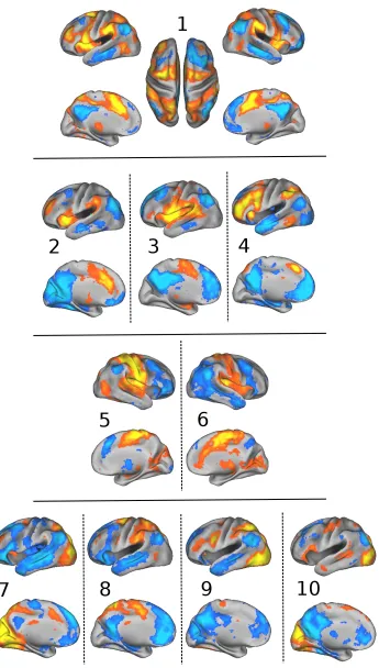
K = 10, λ = 0.3. These ten SCPs are shown in Figure 2.10. We describe them in detail below, and compare to existing knowledge of the spatial extent and behavior

of known task-processing, attention and control systems.

Dorsal Attention SCP Figure 2.10 shows the first SCP defined by the anterior

mid-dle temporal area (aMT), superior parietal lobule (SPL), intra parietal sulcus (IPS)

and the frontal eye fields (FEF)(shown in red), which are known to be part of

the Dorsal Attention (DA) system (Corbetta and Shulman, 2002). These regions

are anti-correlated with the middle temporal gyrus (MTG), inferior parietal lobule

(IPL), medial pre-frontal cortex(mPFC), posterior cingulate cortex (PCC) and

ante-rior frontal operculum, which are part of the default-mode (DM) system (Raichle

et al., 2001)(shown in blue).

Executive Control SCPs SCPs 2, 3 and 4 predominantly show executive task-control

system (red) anti-correlated with different aspects of the DM system (blue). SCP 4

shows the Salience system (Seeley et al., 2007) consisting of dorsal anterior

(51)

(52)

The anti-correlated DM regions include the IPL, PCC and vmPFC. Regions from the

operculum, insula, temporal-parietal junction (TPJ), inferior frontal gyrus (IFG)

and the dACC dominate SCP 5, with anti-correlations to PCC and dmPFC. This SCP

consists of the Cingulo-Opercular (COP) system (Dosenbach et al., 2007) which is

known to de-activate the DM. SCP 6 consists of the aPFC, aI, IPL, and MT, which

form the Fronto Parietal task-control system, anti-correlating with the inferior MTG,

IPL, PCC, mPFC and PHC.

Motor SCPs SCPs 5 and 6 exhibit contributions from the sensori-motor, auditory

and visual areas. Both SCPs show the pre central (prCG) and post central gyrus

(poCG). In SCP 5 the motor areas positively correlate with the superior temporal

gyrus (STG) and posterior insula. The positive correlations in SCP 6 are more

ante-rior within the insula, and a large extent of the cingulum. Anti-correlated regions

include the FP system (aPFC, IPL, aI, ACC) in SCP 5 and aspects of the DM system

in SCP 6.

Visual SCPs SCPs 7, 8, 9 and 10 show four types of connectivity patterns involving

the visual areas. SCP 7 covers the entire visual system, including the medial visual,

lateral visual and higher visual (dorsal attention) areas. SCP 8 shows the higher

visual areas alone. The visual areas are anti-correlated with the DM system in both

the SCPs. SCPs 9 and 10 shows contributions from areas in the lower levels of the

visual hierarchy; the FEF and the prCS are less dominant, while including the lateral

visual areas, which are involved in higher level visual task-processing. Concomitant

with moving down along the hierarchy, we observe changes to the anti-correlated

regions - the involvement of the mPFC is greatly reduced, but the anti-correlation

the posterior cingulate is retained.

Overlap between SCPs The SCPs described above are clearly overlapping, mainly

(53)

Subject Index

SCP Index

20 40 60 80 100 120

2

4 6 8

10 ₀

0.2 0.4

Figure 2.11: Figure illustrating the heterogeneity of the data sample captured by SCPs. The color indicates the extent to which each SCP is present in a individual.

other systems. We note that the PCC and the IPL contribute to most of the SCPs,

which were identified by a prior study as one of the central hubs of connectivity in

the brain (Buckner et al., 2009).

Inter-individual variability Differential presence of the SCPs explains inter

individ-ual variability in functional connectivity. Figure 2.11 shows the strength of presence

of each SCP in every individual. The Sparse Learning approach exploits this

vari-ability; a heterogeneous distribution of the samples in this lower-dimensional space

allows robust identification of the SCPs.

Reproducibility

We evaluate the performance of our algorithm as well as Infomap and ICA based

on repeated split-sample reproducibility. Reproducibility was evaluated for K =

2,4, . . . ,30. In the case of InfoMap, the edge-density was varied between 2% and

40%. This provided sub-graphs varying in number from 4 upto 60, although not equally spaced. Similar to our earlier experiments involving simulated data, we

quantify the comparison between sub-samples using the normalized inner product,

averaged across basis vectors.

The reproducibility of the results is shown in Figure 2.12a, computed for values

(54)

2 4 6 8 10 12 14 16 18 20 22 24 26 28 30 0 0.2 0.4 0.6 0.8 1

Number of Basis (K)

Reproducibility (Normalized Inner Product)

(a) Reproducibility

2 4 6 8 10 12 14 16 18 20 22 24 26 28 30 0

1 2 3 4 5 x 10

6

Number of Basis (K)

Correlation data fit (Error)

(b) Correlation data-fit (Error)

2 4 6 8 10 12 14 16 18 20 22 24 26 28 30 3 4 5 6 7 8

9 x 10

8

Number of Basis (K)

Time−series data fit (Error)

(c) Time-series data-fit (Error)

2 4 6 8 10 12 14 16 18 20 22 24 26 28 30 0 0.1 0.2 0.3 0.4 0.5 0.6

Number of Basis (K)

Spatial Overlap

(d) Spatial Overlap

2 4 6 8 10 12 14 16 18 20 22 24 26 28 30 0 0.05 0.1 0.15 0.2 0.25 0.3 0.35 0.4

Number of Basis (K)

Temporal Correlation

(e) Temporal Correlation

(55)

compared to0.86±0.15for InfoMap,0.79±0.07for Spatial ICA and0.60±0.12for Temporal ICA. InfoMap shows comparable reproducibility with sparse learning (p <

0.4, computed using two-group t-test). Spatial ICA components are as reproducible as Sparse Learning (p < 0.8), while Temporal ICA performs significantly worse

(p < 10−4_{) in terms of reproducibility.}

Data fit

In addition to reproducibility, the data fit (approximation error) of all the methods

to the data was also compared. Given that Sparse Learning and InfoMap use

cor-relation values as input, and ICA methods use time-series as input, we evaluated

the approximation error for both types of input. Let B denote the set of basis

vec-tors output by any of the four methods. Let Yn ∈ RP×T and Xn ∈ RK×T be the

time-series of thenth individual and basis respectively. In the case of Sparse

Learn-ing and InfoMap, the basis-specific time-series Xn can be computed by regressing

the basis B against the individual-specific time-series Yn. Using these values, the

correlation data-fit measure is computed as follows:

Correlation data fit (Error)=

N X n=1

Σn−

ˆ Σn 2 F (2.4) where ˆ

Σn=Bdiag(cn)BT for Sparse Learning (2.5)

Computational Methods for Analysis of Resting State Functional Connectivity and Their Application to Study of Aging

University of Pennsylvania

ScholarlyCommons

Computational Methods for Analysis of Resting

State Functional Connectivity and Their

Application to Study of Aging

Harini Eavani

Computational Methods for Analysis of Resting State Functional

Connectivity and Their Application to Study of Aging

Acknowledgements

ABSTRACT

Contents

List of Tables

List of Figures

Chapter 1

Introduction

1.1

Overview

1.2

Aims of this thesis

1.3

Significance

1.4

Innovation

1.5

rsfMRI data

1.5.1

Datasets

1.5.2

Node definition

1.5.3

Computing the functional connectome

1.6

Organization of this thesis

Chapter 2

Identifying Sparse Connectivity

Patterns

2.1

Introduction

2.2

Literature review

2.3

The Sparse Learning approach

2.3.1

Model formulation

2.3.2

Optimization strategy

2.3.3

Model selection

2.3.4

SCP visualization

2.4

Experiments on simulated data

2.4.1

Generation of simulated data

2.4.2

Performance on simulated data

2.5

SCPs computed from rsfMRI data

2.5.1

Areal graph nodes