* To whom all correspondence should be addressed. E-mail: [email protected]
Hash Algorithm for Finding Associations between Genes
P. Asha1 and S. Srinivasan2
1Research Scholar, Computer Science and Engineering Department, Sathyabama University, Chennai, Tamilnadu, India.
2Professor and Head of the Department, Computer Science & Engineering, Anna University, Regional Centre, Madurai, Tamilnadu, India.
DOI: http://dx.doi.org/10.13005/bbra/1679
(Received: 10 February 2015; accepted: 13 March 2015)
Association rules are those that narrate the relationships prevailing between attributes present in the database. Every rule mining algorithm generate promising items (frequent items) from which, the rules are framed. These rules try to state the items that are most related and how much one item is closer and depending on the other item. But the rules generated are enormous in number. Filtering out the useful patterns becomes difficult. The paper proposes a Hash based algorithm for extracting only the fruitful patterns at a faster rate. The work has been done using R language, and executed in R data mining Toolkit. Comparative study of Hash algorithm with respect to other algorithms shows that the Hash algorithm behaves better than all the other existing algorithms. It has been tested against various benchmark datasets like Adult, Genome, Cancer datasets using various rule interestingness measures like Lift, Confidence, Interest, Support etc.
Key words: Data mining, Associations, Rule Filtration, Interestingness Measures, Genes.
Association rules for example in case of marketing analysis, measures the closeness or relationships that exists between various products brought by some customer. Experimentation on finding the frequent items and then their close associations seems to be difficult and especially when the database size is large1,7,8-9. The algorithm that is used for finding associations2 between items is Apriori Algorithm. Multi-scans is the negative side of Apriori and even with other algorithms6,27. The objective of the work is to propose an effective and efficient mining33,36 of closely associated patterns. This explains on how the technique can find a better place in the area of
medicine and how effectively it has operated over it and proved itself to be better than others. It aims at finding the associations between the human genes, means when one gene gets affected, which are the other genes that do get affected along with it.
Association Rule mining finds wider application in the field of Genomics33, DNA Analysis31, and Bioinformatics, Clone identifications in Software Engineering field, Marketing, and Financial Analysis etc. Both positive and negative rule mining is done, because sometimes the rarest occurring element becomes more important than the positive ones. Finding of effective rules depends on various interestingness measures like Lift, Support, Leverage, Conviction, Confidence etc.
considered are support, confidence, and computation time, number of Rules and Efficiency. Review on existing system
Farah Hanna AL-Zawaidah, Yosef and Hasan proposed that the repeated disk overhead can be reduced by reducing candidate itemset (size related). Associated rules were generated from relational databases and data warehouses using the basic Apriori. It doesn’t tell about the processing speed and the efficiency22 of the rules generated20-21.
Jia Ronga, Huy QuanVua, Rob Lawb, Gang Lia said that different filtering methods were used for rule grouping. Rules generation is applied only to smaller database and especially only for tourism dataset and not for other datasets23-25. Yang Xiang et al25 proposed rule grouping through which we can identify best rules. After which, various distributed and parallel5,10-13 algorithms rooted up.
Xindong et al. worked out BigData concept. They gave HACE26 algorithm for handling such a higher volume and which id heterogeneous in nature27. Chuang H et al. started up with basic hash definitions and its applicability to bigger datasets28
Confidence3-4,18 and support14-19 based croping of items were put forth by Shinji et al. They focused only on the reduction in transaction and not efficient rule generation31. Huan Wu et al. used count method, which followed <itemset, Tids> structure for storing the data. The method counts each candidate itemsets only once. The disadvantage of the system is that, it spends more time for building <itemset, Tids> structure which may never be used for further processing except at the initial phase30.
Jayalakshmi et al. worked on sequential maximal pattern mining and made better pattern hunting,32. Kannika et al. proposed a new method for generating rules based on lift ratio. Interestingness measures33-35 are controlled with minimum level and the generated rules are filtered. Support and confidence are set and lift factor29 is used for filtering the rules.
Hash algorithm
Let D be the database which holds Tr number of transactions (trans). That is, D= {Tr1, Tr2, Tr3…Trm}. Every transaction holds few items
It1, It2, It3… Itm , which could be present in any combination. The item list is denoted by IL = {It1, It2, It3… Itm}. Having set E, such that E Ñ IL then it implies that E Ñ Tr. The association rule is viewed as E => F, where E Ñ IL, F Ñ IL, and E )” F =Ø.
Support supt (E=>F) is given by s% of trans in D containing E U F.
Confidence, confid ( E=>F) is c% of trans in D that contains E U F.
That is,
Then, E=>F is a association rule if Confid (E=>F) e” minconfid,
Matrix Generation
The matrix S={Spq} = m x n, where p=p1, p2,p3… pm and q=q1, q2,q3…qn,
Example 1:
Let us assume that D={Tr1,Tr2,Tr3,Tr4} and IL contain 5 items (represented as It) , which are the one-frequent itemsets present in the database D.
Suppose Tr1 = {It1, It4, It5}, Tr2 = {It2, It3, It4}, Tr3 = {It1, It2}, Tr4 = {It5}.
Then the matrix corresponding to the example 1 is,
Any item’s supt count is calculated by using,
And C1 is the candidate set which consists of 1- Frequent itemsets. Then compare every candidate’s supt count with the minimum (min-sup) support threshold. Supt_count { Itq} >= min-sup and if so then we conclude that Itq ª L1 (Level 1: 1-Freq_itemset). The next step is to frame 2-Frequent itemsets and then 3-Frequent itemsets etc… until the candidate satisfies the min-sup specified.
,
and the algorithm proceeds and terminates when no further combinations can be made. Then finally
where L contains the complete set of frequent items. After which, the association rules are generated. Remember every sub-set present in the frequent item set should be frequent too. That is,
i ª L : Lk – {i} ª L
Methodology
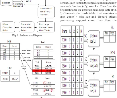
Initially, scan the dataset and create candidate itemset. From that create a hash table for 2 itemsets and then find out large itemsets from the hash table. From the frequent itemsets retrieved
now we make association rules. As it may produce many numbers of rules which may be redundant and insignificant, it is a must to remove all those and get only the best rules. Finally we can group similar rules (Fig. 1).
The proposed methodology tries to overcome the problems of the existing system. It contains four modules:
Frequent itemset generation
Choose the input dataset and minimum support count, min_sup. Create candidate item-1 and Hash table for generating candidate item -2.
Then create large itemset from candidate item 1and make large item 2 from hash table -1.Next create Hash table -2 from Hash table-1. Repeat the process for creating hash table and large itemset.
Hash table
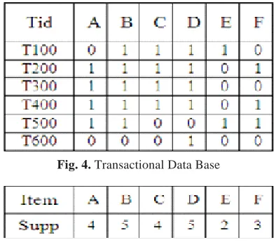
Read the data for candidate item 2 from dataset at the 1st scan. Then we create hash data structure with min_sup and item name (Fig.2) for 2 itemset. Each item in the separate column and row uses hash function (x*y) mod Ln. Then from the first hash table we generate next hash table (Fig. 3).Generate the hash table that contains a supt_count > min_sup and discard others possessing support count less than the
Fig. 1. Architecture Diagram
min_support count. At the same time truncate the transaction with no frequent item (marked with red color in Fig. 2). Before creating the hash table element, remove the item having less support count from the transaction. (marked with blue circles in Fig. 2).
Rule generation
Then we try to retrieve the rules that were associated based the resultant frequent items. After which, these rules are filtered and refined using various interestingness measures like Confidence, Lift, Leverage, Laplace, Interest Factor etc7
Grouping rules
Similar rules are joined together based on the Rule Head. Rule Head contains the same value group that rules into one. Hence we try to reduce the generated rules based on grouping.
Hash algorithm
The algorithm is as follows: Hs_alg()
{
The algorithm starts with a candidate itemset of one.
Ck: Candidate item set of size k L1<- frequent 1-itemsets
Generate candidate for every Lk do begin Ck+1 <- candidate(Lk) #New candidates Join Step: Ck is generated by joining Lk-1 with itself For all transactions t “D do begin
Ck <- subset [Ck, t] #Candidates contained in t
For all candidates c “Ct do c. count++;
Prune Step: Any (k-1) –Subset of infrequent itemset must be infrequent.
Lk {c “C | c.count>= minsup} Final Lkas frequent item from dataset. }
Grp_ru() //// Grouping similar rules
{
Rmerge = merge(RevDup(G1), RevDup(G2)) MG = group_by_RHS(Rmerge)
For each G “ MG { agent = find_agent(G)
DR = sort_by_4condition(agent) Return (DR)
}
Rul_fil() //Rules generated after filtering { R=Fk> {Confidence, Lift, Leverage, Interest Factor}
}
/// Sample Code
colnames(spm)<-c(“x”) while(j<=m)
{ candidateset<-as.data.frame(itemset[j,]) #print(candidateset)
counttot<-0 i<-1 counttot<-sp(itemset,data,sc) spm[j,]<-counttot j<-j+1 } rt<-as.data.frame(cbind(itemset,spm)) sorted<-rt[order(-rt$x),]
Rule Interestingness measures and Grouping
Lh means the instances present at the left (LHS) hand side of a rule and Rh means the instances at its right (RHS) hand side. Let Proba represents the probabilty.
1. Confid = P (Lh U Rh) / P (Lh).
2. Supt = P (Lh U Rh) / Ntotal, where Ntotal represents the total number of instances.
3. Lift (Lh U Rh) = count (Lh U Rh) / count (Lh) * supp (Rh) 4. Leverage (Lh->Rh) = supp (Lh U Rh) - supp (Lh)*supp(Rh)
Example
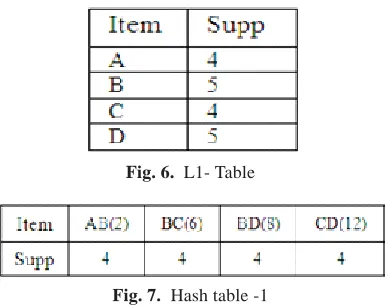
Consider Fig. 4 as an example Transaction database. Find the candidate item set -1 using normal Apriori algorithm (Fig. 5). Next generate L1(Fig. 6) from candidate item -1 with itemset satisfying a supt_count value >= min_sup and other itemsets were removed. After this step create hash table for each itemset, due to the presence of large number of itemset combinations in item
set-Fig. 4. Transactional Data Base
2, which consumes too much time for generation of large item set -2.
For the next iteration we need 3 combinations. Remove transaction T500 because it has only one large 2-itemset. Transaction T300 contains A only once, B and D thrice in 3 combination pattern. So we can remove A from the transaction, because we need more than 2 combinations in next step. Similarly, we delete A, F in transaction 200 and 400, E in transaction 100 and hence in this way we can create next step of data easily using the hash table (Fig. 9). Hence the final step would be a simplified database and as a result we achieve data reduction.
Sparse matrix representation
Let T1, T2….Tn represent the patient number and VWF, MSH2 etc., represent the Colon-Cancer infected gene [17], [20]. The value 1 indicates the presence of infected gene for that particular patient. And the input database contains approximately 2 lakh records and hence applying the mining algorithm to it would be too difficult. Hence to reduce that database into a smaller size we try to represent it in a vertical format, stated as, for example take Gene wise listings, say VWF, now find out the for which all patients it is present. Proceeding like this would probably reduce the database size as repetitive infected gene would appear in the database.
Now apply the Apriori Algorithm. Find 1 (individual) frequently occurring gene from which two closely associated genes are generated. Next from the two- combinations generate the three combinations, that is, the three individual genes that are in close relation and iterate the procedure for multiple combinations and in every stage sum up its presence in the database. Next in every stage filter only the combination of genes which carries
Fig. 6. L1- Table
Fig. 7. Hash table -1
Fig. 8. L2-table
Fig. 9. Data base for 3 item set
First create a hash table with hash function H(X) =(X*Y) MOD size (L1*L1). Based on the hash function, item combinations have some specific place for them. The Hash table defines itself with a structure which looks like the one depicted in Fig. 4. Hash value is specified within the bracket of every itemset combination. Then check every itemset for its supt_count, and those that satisfy their min_sup retains and others are pruned. Assume the minimum support to be 4.Here the transaction T600 contains item D and only this has a support count greater than minimum. Then the possible combinations for next iteration (two-item combinations) are AB, CD etc. From this combination create hash table -1(Fig. 7) and generate L2-table from hash table -1(Fig. 8).
a supt_ count >= user specified threshold. Hence, our final resultant would be the best combination, i.e. only the frequently occurring [13], [15], [16], [18], [19] infected genes would sustain as a result of the algorithm. Next generate the association rules from resultant data. Now enormous amount of rules might exist which would be unproductive, redundant or insignificant.
So try to eliminate the unfruitful elements and retain only the most promising rules. Such a technique is termed as Filtration of rules.
Rule interestingness measures
There are two basic Interestingness Measures, Subjective and Objective measures. Subjective measures of Interestingness states the belief of the user. It is categorized into two, namely Actionability and Unexpected. Unexpected measures states that the pattern found while discovery may be much astonishing and useful to the user. Actionability measure is that the user act over the pattern to gain advantage of it. Objective measures work on the data and the structure of rule in a discovery procedure. Support and
Confidence are objective measures. It generates best rules which may be or may not be much interesting to the user. So, to obtain the best and highly interesting rule, it is important to have a combined format, which is the combination of Subjective and Objective measures.
Rule Interest Measures
Finding the best and top rules seems to the biggest motto of rule mining. Basically used measures are: Confidence, Support.
Discriminality is one other measure which is used to infer how much the rules are able to distinguish/classify one category from the other. 1- (Proba(Lh U Rh) - Proba(Lh U Rh) ) / (Ntotal -Proba(Rh))
If discriminality is 1 then that implies a strong classification has been made. That is Proba(Lh) = Proba(Lh U Rh).
Piatetsky-Shapiro Measure
Gregory Piatetsky-Shapiro has put forth three criteria that every interestingness (Intr) measure of a rule should comply with.
Criteria 1:
Intrst measure should be zero if Proba(Lh U Rh) = (Proba(Lh) * Proba(Rh)) / Ntotal
Criteria 2:
Intrst measure must be upgraded monotonically along with Proba(Lh U Rh)
Table 2. Computation time, memory usage -Transactions
Trans Freq. Ass. Exec Memory Conf Items Rule Count Time Usage
5 69 437 81 1116 50 10 104 1011 138 362 50 15 65 351 58 647 50 20 59 290 49 511 50
Table 1. Calculation of execution time, Memory usage - Support
Supp Freq. Ass. Exec Memory Conf Items Rule Count Time Usage
0.2 77 356 62 712 50 0.4 32 301 54 66 50
0.6 30 29 27 16 50
0.8 21 3 5 7 50
Table 3. Rules after removal of Redundancy
Total no of Rules when Support = 31% Before Filtering After Filtering
120 26
Criteria 3:
Intrst measure must be degraded monotonically along with every Proba(Lh) and Proba(Rh) Intrst is defined as, Intrst = Proba(Lh U Rh) -(Proba(Lh) * Proba(R)) / Ntotal
Usually the value of Intrst is >0.
If Intrst = 0, then the chance is better than the rule obtained and if Intrst = <0, then the chance is somewhat (quiet) better than the rule obtained.
Performance analysis
The work has been implemented using R language. Table I shows the characteristics of our infected-gene dataset, which displays the set of association rules retrieved, req-items generated,
total execution time, memory usage with respect to different support thresholds and Table II with respect to Transactions.
Table III shows the total number of rules generated when the support=0.09. Here, we can observe that the number of rules has been reduced from 120 to 26 after redundancy removal and refinement by the various rule interestingness measures. That is, if support count increases, the number of rules generated also increases. But after certain range, the number of rules generated can also be nil. For the support value > 4/6/8, no rules were generated.
Fig. 12. Rule with conclusion =”VWF”
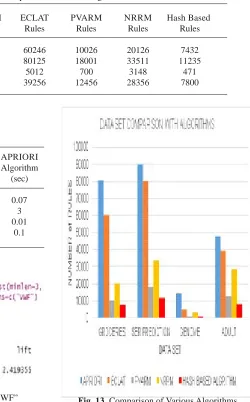
Table 4. Comparison of Various Algorithms
Dataset APRIORI ECLAT PVARM NRRM Hash Based Rules Rules Rules Rules Rules
Groceries 80856 60246 10026 20126 7432 Ser Prediction 90032 80125 18001 33511 11235 Genome 14256 5012 700 3148 471 Adult 48000 39256 12456 28356 7800
Fig. 13. Comparison of Various Algorithms
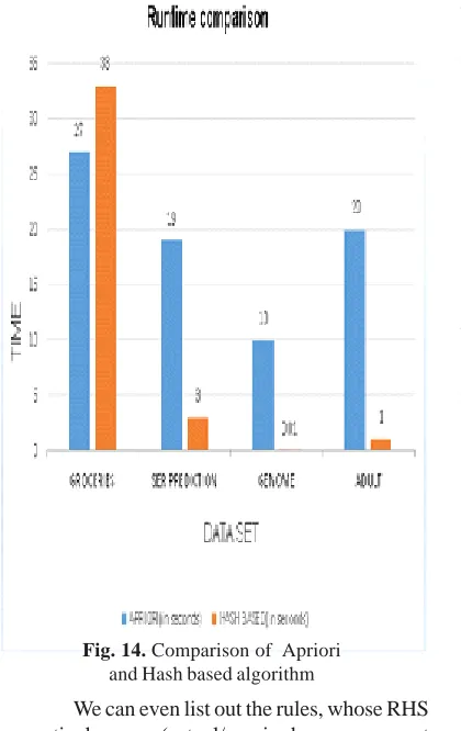
Table 5. Execution time
Dataset Hash Based APRIORI APRIORI Algorithm
(sec) (sec)
Groceries 29 0.07
Ser Prediction 19 3
Genome 10 0.01
Fig. 14. Comparison of Apriori and Hash based algorithm
We can even list out the rules, whose RHS is a particular gene, (actual/required gene we expect to know about) that is the resultant gene received as a result of various infected gene combinations. In Fig. 12, we try to list the rules where RHS=VWF. The resultant is only one rule that has satisfied the specified constraint.
Comparative study of Apriori, Éclat mining algorithm, PVARM(Partition based Validation for Association Rule Mining), NRRM (non-redundant rules method) and Hash Based with respect to various datasets like adult, genome, groceries and SER prediction are done. The reason behind these dataset selection is that, these dataset have different transaction size, item size (Table IV). The Fig.13 shows bar chart of comparison of various algorithms. Horizontal axis has each algorithm in its side and y axis has support level 0 to 1 Lakh. In this study we fixed minimum confidence=50% and lift=20% and monitored their execution time. From Fig 13, we infer that the Hash algorithm performs well when compared to all others, with most interesting rules and
non-redundant rules.
Table V shows the time taken by the Apriori and Hash based algorithm, for the entire data mining task
From Fig. 14 we can conclude that Hash algorithm performs better than the Apriori, that is the entire computation withy very less time and excels even with larger datasets (Table V).
CONCLUSION
We conclude that, the Hash algorithm has performed well based on the performance analysis stated with various parameters. The algorithm scales well for bigger databases too. We have made a thorough analysis of gene associations and with lesser time and accurate combinations and frequencies.
REFERENCES
1. R. Agrawal et al., “Fast Discovery of Association Rules,” Advances in Knowledge Discovery and Data Mining, U. Fayyad et al.,eds., AAAI Press, Menlo Park, Calif., 1996, pp. 307–328. 2. R. Agrawal and J.C. Shafer , “Parallel Mining of
Association Rules,” Distributed Systems Online March 2004.
3. S. Brin et al., “Dynamic Itemset Counting and Implication Rules for Market Basket Data,” Proc. ACM SIGMOD Conf. Management of Data, ACM Press, New York, 1997, pp. 255– 264.
4. Kun-Ming Yu, Jiayi Zhou, Tzung-Pei Hong, Jia-Ling Zhou, “A load-balanced distributed parallel mining algorithm,” Expert Systems with Applications, 37 (2010),pp. 2459–2464. 5. Einakian and Ghanbari, M., “Parallel
implementation of association rules in data mining,” System Theory, SSST ’06, IEEE Proceeding of the Thirty-Eighth Southeastern Symposium, 2006, pp. 21–26.
6. Oded Maimon and Lior Rokach, The Data Mining and Knowledge Discovery Handbook, Springer, 2009 Edition.
7. A. Savasere , E. Omiecinski, and S.B. Navathe, “An Efficient Algorithm for Mining Association Rules in Large Databases,”Proc. 21st Int’l Conf. Very Large Databases.
8. Zaki, M. J., “Parallel and distributed association mining: A survey,” IEEE Concurrency, Special Issue on Parallel Mechanisms for Data Mining, 7(4):14—25, December 1999.
for mining association rules,” Proceedings of the 20th international conference on very large databases 1994, pp. 487– 499.
10. P.Asha, Dr.T.Jebarajan, “Analyzing the sequential and Parallel ARM Algorithms and its impact in Grid Computing Environments,” International Journal of Advanced Computing,Vol.36, No. 1, pp.1109-1114. 11. Cheung, D. W., Lee, S. D., & Xiao, Y., “Effect of
data skewness and workload balance in parallel datamining,” IEEE Transactions on Knowledge and Data Engineering, 2002; 14(3); 498–514. 12. Zaki, M. J., Ogihara, M., Parthasarathy, S.,
“Parallel data mining for association rules on shared-memory multi-processors,” Proceedings of the ACM/IEEE Conference on Supercomputing, 1996.
13. Cai,R., Tung, A.K.H., Zhang,Z., & Hao, Z.”What is unequal among the equals? Ranking equivalent rules from gene expression data”, IEEE Transactions on Knowledge and Data Engineering, 2011; 23(11), 1735-1747. 14. Shichao Zhang, Xindong Wu, Chengqi Zhang,
Jingli Lu S. “Computing the minimum-support for mining frequent patterns,” Knowledge and Information Systems,15(2), 2008: 233-257. 15. Cai, Ruichu, Zhifeng Hao, Wen Wen, and Lijuan
Wang. “Regularized Gaussian Mixture Model based discretization for gene expression data association mining.” Applied Intelligence (2013): 1-7.
16. Zhao, Yuhai, Guoren Wang, Yuan Li, and Zhanghui Wang. “Finding novel diagnostic gene patterns based on interesting non-redundant contrast sequence rules.” In Data Mining (ICDM), 2011 IEEE 11th International Conference on, pp. 972-981. IEEE, 2011. 17. Wang, MeiHua, XiongBin Su, FuMing Liu, and
RuiChu Cai. “A cancer classification method based on association rules.” In Fuzzy Systems and Knowledge Discovery (FSKD), 2012 9th International Conference on, pp. 1094-1098. IEEE, 2012.
18. Wang, Meihua, Shumin Wu, and Ruichu Cai. “Two novel interestingness measures for gene association rule mining.” Neural Computing and Applications: 1-7.
19. Jiang, Daxin, Chun Tang, and Aidong Zhang. “Cluster analysis for gene expression data: A survey.” Knowledge and Data Engineering, IEEE Transactions on 16, no. 11 (2004): 1370-1386. 20. Glaab, Enrico, Jaume Bacardit, Jonathan M. Garibaldi, and Natalio Krasnogor. “Using Rule-Based Machine Learning for Candidate Disease Gene Prioritization and Sample Classification of Cancer Gene Expression Data.” PloS one 7,
no. 7 (2012): e39932.
21. Farah Hanna AL-Zawaidah, Yosef Hasan, “An Improved Algorithm for Mining Association Rules in Large Databases,” World of Computer Science and Information Technology Journal (WCSIT), 2011, pp. 487-499.
22. Bouker, R. Saidi, S. B. Yahia, M. E. Nguifo, “Ranking and selecting association rules based on dominance relationship,” Proceedings of the International MultiConference of Engineers and Computer Scientists 2013 Vol I, IMECS 2013, March 13 - 15, 2013, Hong Kong .
23. Jia Ronga, Huy Quan Vua, Rob Lawb, GangLia ,”A behavioral analysis of web sharers and browsers in Hong Kong using targeted association rule mining,” Tourism Management,
2012: 33(4), pp. 731-740.
24. Phaichayon, Nittaya Kerdprasop, and Kittisak Kerdprasop,”Dissimilar Rule Mining and Ranking Technique for Associative Classification,” In the Proceedings of the International MultiConference of Engineers and Computer Scientists, Vol I, IMECS 2013, March 13 - 15, 2013, Hong Kong.
25. Yang Xiang Philip, Payne Kun Huang, “Transactional Database Transformation and Its Application in Prioritizing Human Disease Genes,” IEEE/ACM Transactions On Computational Biology And Bioinformatics, 2012: 9(1).
26. Xindong Wu, Xing Quan Zhu, Gong-Qing Wu, and Wei Ding, “Data Mining with Big Data,”
IEEE Transactions On Knowledge And Data Engineering, 2014;26(1).
27. Ms. Sushma Bhasgi, Dr.Parag Kulkarni ,”Multilevel Association rule based data mining,”
International Journal of Advances in Computing and Information Researches, ISSN:2277-4068,
1(2), April 2012.
28. W. Hranchotchuang, T. Rakthanmanon, K. Waiyamai, “Using Hash Based Apriori Algorithm to Reduce Candidate Itemset-2 for Mining Association Rule,” IJCSI International Journal of Computer Science Issues, 2009: 6: 35-4
29. S. Bouker, R. Saidi, S. B. Yahia, M. E. Nguifo, “An Effective Hash Based Algorithm for Mining Association Rules,” In Proceedings of the 24th IEEE International Conference on Tools with Artificial Intelligence, 2012.
31. Shinji Funjiwara, Jeffrey D. Ullman, Rajeev Motwani, “Dynamic Miss Counting Algorithm Finding Implication and Similarity Rules with Confidence Pruning,” In Proceedings of the 1st National Conference on Computing and Information Technology, 2005, pp 24–25. 32. Jayalakshmi, V. Vidhya, Krishnamurthy,
Kannan, “Frequent Itemset Generation using Double Hashing Technique,” International Conference On Modeling Optimization And Computing, 2012: 38; 1467–1478.
33. Ramesh kumar K, Sambath M , Ravi S, “Relevant association rule mining from medical dataset using new irrelevant rule elimination technique, “ International Conference on Information Communication and Embedded Systems (ICICES), 2013 21-22 Feb. 2013.
34. Anand H.S, Vinod Chandra S.S, “Applying Correlation Threshold on Apriori Algorithm, “ IEEE International Conference on Emerging Trends in Computing, Communication and Nanotechnology, (ICECCN 2013).
35. Kannika NiraiVaani, M. Ramaraj, “An integrated approach to derive effective rules from association rule mining using genetic algorithm,” International Conference on Pattern Recognition, Informatics and Mobile Engineering (PRIME), 21-22 Feb. 2013.