Geometric Unification of Electromagnetism and Gravitation
Raymond J. Beach
Lawrence Livermore National Laboratory, L-465, 7000 East Avenue, Livermore, CA 94551 E-mail: [email protected]
Using four equations, a recently proposed classical field theory that geometrically couples electromagnetism to gravitation in a fundamentally new way is reviewed. Maxwell’s field equations are a consequence of the new theory as are Einstein’s field equations augmented by a term that can replicate both dark matter and dark energy. To emphasize the unification brought to electromagnetic and gravitational phenomena by the new theory specific solutions are investigated: a spherically-symmetric charged particle solution, a cosmological solution representing a homogeneous and isotropic universe, and solutions representing electromagnetic and gravitational waves. A unique feature of the new theory is that both charge and mass density are treated as dynamic fields, this as opposed to their treatment in the classical Maxwell and Einstein field equations where they are introduced as external entities. This feature suggests a procedure for quantizing the mass, charge and angular momentum that characterize particle-like solutions. Finally, antimatter, which is naturally accommodated by the new theory, and its interaction with a gravitational field is investigated.
(key words: unified field theory; electromagnetism; Maxwell’s equations; gravitation; General Relativity; Einstein’s field equations; gravitational radiation; hidden variable; dark matter; dark
energy)
Introduction
Electromagnetic and gravitational fields both have long range interactions characterized by speed of light propagation, similarities that suggest these fields should be coupled together at the classical physics level. Although this coupling or unification is a well-worn problem with many potential solutions having been proposed, it is fair to say that there is still no generally accepted classical field theory that can explain both electromagnetism and gravitation in a coupled or unified framework.i The existence of electromagnetic and gravitational fields are generally
understood to be distinct and independent with electromagnetism being described by the Maxwell field equations which treat gravitational fields as an external entity when necessary, and gravitational fields being described by the Einstein field equations which treat electromagnetic fields as an external entity when necessary. The purpose of this manuscript is to reassess the connection between electromagnetism and gravitation using an entirely new approach.
Assuming the geometry of nature is Riemannian with four dimensions, the following four equations provide a description of classical physics at the level of the Maxwell and Einstein Field Equations (M&EFEs),ii but then go further by reconciling gravity and electromagnetism
;
Fμν κ =a Rλ λκμν (1)
c
a Rλ λν =ρuν (2)
1 u uλ
λ = − (3)
; 1
0 4
mu uμ ν F Fμλ ν λ g F Fμν ρσ ρσ ν ρ
+ − =
(4)
Both equations (1) and (2) are new, as is the vector field aλ that appears in them and serves to couple gravity to electromagnetism. Equation (1) couples the Maxwell tensorFμν to the Riemann-Christoffel (R-C) tensor Rλκμν. Equations (2) couples the Ricci Tensor Rλν to the coulombic current density ρcuν. Supplementing these first two equations are equations (3) and
describes the motion of both the charge density field ρc and the mass density field ρm, which
are assumed to be comoving. Equation (4) describes the conservation of energy and momentum for a specific choice of energy-momentum tensor. Much of the discussion that follows will be focused on describing solutions to these equations and demonstrating that such solutions are consistent with those of the classical M&EFEs, but then go further by unifying electromagnetic and gravitational phenomena. Taken together, the four field equations are used to axiomatically build up a description of nature in terms of the six dynamic fields described in Table I.
Table I. Dynamic fields
Field Description Number of components
gμν Metric tensor 10
Fμν Maxwell tensor 6
uλ Four-velocity 4
aλ Four-vector coupling electromagnetism to
gravitation 4
ρc Charge density 1
ρm Mass density 1
Total number of independent field components 26
the theory; a development which opens the possibility of quantizing such solutions for charge, mass and angular momentum using a set of self-consistency equations that flow from the analysis. Next a cosmological solution representing a homogenous and isotropic universe is analyzed, and the time dependence of the cosmic scale factor derived. Two radiative solutions representing electromagnetic and gravitational waves are then developed with an emphasis on the unification that the theory brings to these phenomena. Next is a discussion of antimatter, covering how it is accommodated by the new theory and how it interacts with a gravitational field. Finally, to gain insight into the numerical solution of the fundamental field equations (1) through (4), an analysis of the Cauchy initial value problem as it applies to them is given in Appendix II.
In this manuscript geometric units are used throughout and the metric tensor has signature [+,+,+,-]. Commas before tensor indices indicate ordinary derivatives while semicolons before tensor indices indicate covariant derivatives. Spatial indices run from 1 to 3, with 4 the time index. For the definitions of the R-C curvature tensor and the Ricci tensor, the conventions used by Weinberg are followed.iii
Maxwell’s equations from Fμν;κ = a Rλ λκμν and =
ν λ ν
c λ
ρu a R
Equations (1) and (2) which relate the Maxwell tensor derivatives to the R-C tensor and the charge current density to the Ricci tensor, respectively, are the fundamental relationships from which all of Maxwell’s equations flow. Maxwell’s homogenous equation is derived using the algebraic property of the R-C tensor
0
Rλκμν +Rλμνκ +Rλνκμ = . (5)
Contracting (5) withaλ gives,
0
a Rλ λκμν +a Rλ λμνκ +a Rλ λνκμ = . (6)
; ; ; 0
Fμν κ +Fνκ μ+Fκμ ν = , (7)
which is Maxwell’s homogenous equation. Maxwell’s inhomogeneous equation follows from (1) by contracting its μ and κ indices
;
Fμν a Rλ ν
μ = − λ . (8)
Making the connection between the RHS of (8) and the coulombic current density ρcuν ≡Jν
using (2) then gives the conventional Maxwell-Einstein version of Maxwell’s inhomogeneous equation
; c ( )
Fμνμ = −ρ uν ≡ −Jν . (9)
Because Fμνis antisymmetric, the identityFμν; ;μ ν =0 is forced, which in turn forces the coulombic charge to be a conserved quantity
( ) (
cu ; a R)
; 0ν λ ν
λ
ν ν
ρ = = . (10)
Using equations (2) and (3), the coulombic charge density can be solved for in terms of a uλ, λ and the Ricci tensor,
c
a R a R or a R u
λ ν σ
λ σν
λ ν
λ ν ρ
±
= −
. (11)
In the forgoing development, only equations (1), (2) and (3) are fundamental to the new theory. Maxwell’s equations (7) and (9), the conservation of the charge (10), and the solution for the coulombic charge density (11), are all consequences of (1), (2) and (3), and the properties of the R-C curvature tensor. These additional equations all represent constraints; any solution of (1), (2) and (3) must also satisfy (7), (9), (10) and (11).
and the charge density to the metric tensor through (2). Much of the analysis and discussion that follows will be focused on the impact of aλ and how it drives the development of a classical field theory that encompasses the physics covered by the M&EFEs, but then goes further by unifying gravitational and electromagnetic phenomena.
A classical field theory that unifies electromagnetism and gravitation
As shown in the preceding section, equations (1), (2) and (3) when combined with the properties of the R-C tensor provide a basis for deriving Maxwell’s homogenous and inhomogeneous equations in curved space-time. Taking the source terms of the gravitational and electromagnetic fields, ρm and ρc, respectively, as dynamic fields to be solved for, a classical
field theory of gravitation and electromagnetism that is logically consistent with the requirements of general covariance is possible. For a theory to be logically consistent with the requirements of general covariance, the N dynamical field components of the theory must be underdetermined by N-4 independent equations, the remaining 4 degrees of freedom representing the freedom in the choice of coordinate system.
Table I lists the 6 dynamic fields of the theory along with the number of independent components that comprise each field, yielding a total of 26 independent field components. Now consider the last of the theory’s fundamental equations, equation (4), the energy and momentum conservation equation
; 1
0 4
mu uμ ν F Fμλ ν λ g F Fμν ρσ ρσ ν ρ
+ − =
. (4)
The specific form of the energy-momentum tensor in (4) ensures that ρm is conserved and that
there is a Lorentz force law. These two dependent equations are derived by first contracting (4) with uμ which leads to the conservation of mass
(
mu)
; 0ν ν
ρ = , (12)
m c Du
u F D
μ
λ μ λ
ρ ρ
τ = (13)
where ;
Du
u u D
μ
μ σ
σ
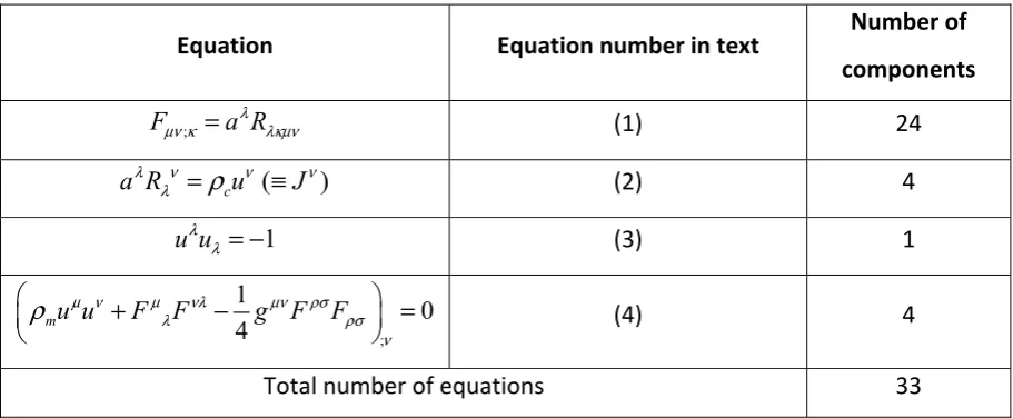
τ ≡ . A more complete outline of the derivation of (12) and (13) is given in the Appendix I. Table II collects and summarizes the four fundamental equations of the new theory, along with the number of components of each equation.
Table II. Fundamental equations
Equation Equation number in text Number of
components
;
Fμν κ =a Rλ λκμν (1) 24
( ) c
a Rλ λν =ρuν ≡Jν (2) 4
1
u uλ λ = − (3) 1
;
1 0
4
mu uμ ν F Fμλ νλ g F Fμν ρσ ρσ ν ρ
+ − =
(4) 4
Total number of equations 33
Table III. Dependent equations
Equation Equation number
in text Derivation
Number of
components
; ; ; 0
Fμν κ+Fνκ μ +Fκμ ν = (7)
(1) and
0
Rλκμν +Rλμνκ +Rλνκμ = 4
( ) (
cu ; a R)
; 0ν λ ν
λ
ν ν
ρ = = (10) (1) and (2) 1
c
a R a R or a R u
λ ν σ
λ σν
λ ν
λ ν ρ
±
= −
(11) (2) and (3) 1
(
mu)
; 0ν ν
ρ = (12) (4), (3) and (7) 1
m c
Du
u F D
μ
λ μ λ
ρ ρ
τ = (13) (4), (3)and (12) 4
Total number of equations 11
The 11 dependent constraint equations listed in Table III mean that of 33 fundamental component equations listed in Table II, only 33-11=22 are independent. These 22 independent equations satisfy the requirements of general covariance for determining the 26 independent field components of Table I. The remaining four degrees of freedom in the solution representing the four degrees of freedom in choosing a coordinate system. To further elucidate the mathematical content of the fundamental field equations (1) through (4), an outline of their solution when viewed as a Cauchy initial value problem is presented in Appendix II.
Symmetries of the fundamental field equations
c c
m m
u u
a a
F F
g g
λ λ
λ λ
μν μν
μν μν
ρ ρ
ρ ρ
−
− →
−
, (14)
the second corresponds to a matter-to-antimatter transformation as will be discussed and justified later
c c
m m
u u
a a
F F
g g
λ λ
λ λ
μν μν
μν μν
ρ ρ
ρ ρ
−
−
− →
, (15)
and the third symmetry is the product of the first two
c c
m m
u u
a a
F F
g g
λ λ
λ λ
μν μν
μν μν
ρ ρ
ρ ρ
−
→
−
. (16)
All three transformations (14) through (16) leave the fundamental equations (1) through (4) unchanged. Adding an identity transformation to the symmetries (14) through (16) forms a group, the Klein-4 group with the product of any two of the symmetries (14) through (16) giving the remaining symmetry. Note that among the fundamental fields of the theory, only gμν and
m
ρ are unchanged by the symmetry transformations, a fact that will be useful later for defining
Is Electromagnetism as defined by the new theory compatible with the classical Maxwell’s
equations?
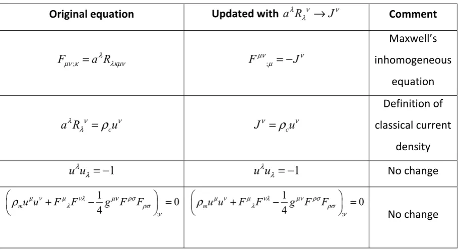
Equations (1) and (2) are the most important concepts being proposed in this manuscript, fundamentally tying the Maxwell tensor and charge density to the R-C curvature tensor and thereby unifying electromagnetism with gravitation. The cost of this unification is the introduction of a new field aλ, a field that has no counterpart in classical physics but in the new theory serves to couple electromagnetic and gravitational phenomena. The unification that ensues puts electromagnetic phenomena on par with gravitational phenomena, with both intrinsically tied to nonzero curvatures. On the surface this central role for nonzero curvature in all electromagnetic phenomena might be construed as problematic due to the prevalent view today that electromagnetic phenomena can exist in flat space-time. However, looking a little deeper it is not hard to see the connection between the new theory that requires a nonzero curvature for all electromagnetic phenomena and the classical Maxwell theory that works in flat space-time. If one were not aware of the vector field aλ, but recognized the existence of the coulombic current density as is the view today, then that part of the new theory not directly connected to aλis exactly the classical Maxell theory. To see this, consider the equations in Tables II and III that result from replacing a Rλ λν with the classical coulombic current density, which is just a statement of fundamental equation (2). The before and after equations with this substitution are shown in Tables VI and VII. The equations updated with the substitution
Table VI. Fundamental equations from Table II with a Rλ λν →Jν
Original equation Updated with a Rλ λν →Jν Comment
;
Fμν κ =a Rλ λκμν Fμν;μ = −Jν
Maxwell’s inhomogeneous
equation
c a Rλ ν uν
λ =ρ Jν =ρcuν
Definition of classical current
density
1 u uλ
λ = − u uλ λ = −1 No change
;
1
0 4
mu uμ ν F Fμλ νλ g F Fμν ρσ ρσ ν ρ
+ − =
;
1
0 4
mu uμ ν F Fμλ νλ g F Fμν ρσ ρσ ν ρ
+ − =
No change
Table VII. Dependent equations from Table III with a Rλ λν →Jν
Original equation Updated witha Rλ λν →Jν Comment
; ; ; 0
Fμν κ +Fνκ μ+Fκμ ν = Fμν κ; +Fνκ μ; +Fκμ ν; =0 No change
( ) (
cu ; a R)
; 0ν λ ν
λ
ν ν
ρ = = Jν;ν =0
Conservation of charge
c
a R a R or a R u
λ ν σ
λ σν
λ ν
λ ν ρ
±
= −
c c
ρ =ρ Trivial identity
(
mu)
; 0ν ν
ρ =
(
ρmuν)
;ν =0 No changem c
Du
u F D
μ
λ μ λ
ρ ρ
τ = m c
Du
u F D
μ
λ μ λ
ρ ρ
In considering the new theory, one might view classical physics at the level of the classical Maxwell field equations as incomplete, there being a hidden field aλ that has gone unrecognized. So while the classical Maxwell equations are a consequence of the new theory, they are not the entire story as solutions to the classical Maxwell equations can exist in flat space-time, a situation that can only be an approximation of solutions to the entire set of field equations (1) through (4) which strictly require curved space-time for electromagnetic phenomena.
How do the Einstein field equations comport with the new theory?
While evident from the preceding discussion that Maxwell’s field equations and the classical physics that flows from them are derivable from the fundamental equations (1) through (4), at this point it is not obvious that the same can be said of Einstein’s field equations. The particle-like solution to be analyzed in the following section demonstrates that the Reissner-Nordstrom metric is an exact solution of the fundamental field equations (1) through (4), thus establishing that the new theory and classical General Relativity support the same solutions, at least in the case of spherical symmetry. But one must go further to determine if Einstein’s field equations are in fact derivable from the fundamental equations of the new theory. To investigate this question, I start by considering equation (4). An immediate consequence of (4) with its vanishing covariant divergence is that a number of trivial tensor equations can be written down relating the covariant divergence of the energy-momentum tensor used in (4) to various geometric quantities. The simplest example of such a tensor equation is
; ;
Gμνν =αTμνν (17)
where 1
2
Gμν ≡Rμν − g Rμν is the Einstein tensor, α is an arbitrary constant, and Tμν is the
energy-momentum tensor defined in (4)
1 4 m
While (17) is rigorously true, it’s trivially satisfied because both sides are independently 0, the left being 0 by the Bianchi identity and the right by fundamental equation (4). However, an immediate consequence of equation (17) on taking the anti-covariant derivative of both sides is
Gμν =αTμν + Λμν , (19)
where Λμν is a symmetric tensor field
μν νμ
Λ = Λ , (20)
and is forced to have vanishing covariant divergence
; 0
μν ν
Λ = . (21)
In the view being put forth here, (19) is satisfied by any solution of fundamental fields that satisfy equation (4). However, (19) by itself contains no useful information. To see this, consider that (19) is trivially satisfied for any Gμν and Tμν that go with any specific solution to equations (1) through (4), and any value for the constantα by taking Λ =μν Gμν −αTμν. This also demonstrates that the specific choice for the value of α is completely arbitrary and without physical significance; a change in the value of α is absorbed by a change to Λμν such that (19) remains satisfied. This discussion should make clear that (19) is of no value when attempting to find a solution to the fundamental fields. To gain a deeper understanding of how (19) fits into the new theory set α = −1, again a choice having no physical significance but one that is convenient because equation (19), except for the appearance of Λμν, reduces to the Einstein field equations in this case, i.e.,
Gμν = −Tμν + Λμν . (22)
It is important to note that equation (22) with its auxiliary conditions (20) and (21) is a consequence of only the fundamental field equation (4) and the properties of the R-C tensor. With questions today regarding the validity of classical General Relativity beyond the confines of our own solar system,iv the most interesting aspect of Λμνin (22) is that it can represent both
dark matter and dark energy. Today such terms are appended to the energy-momentum tensor of Einstein’s field equations in an ad hoc manner to explain, for example, the flattening of rotational-velocity curves observed on galactic scales, and the accelerating expansion of the universe. However, in the approach being proposed here such terms are a logical consequence of the fundamental field equation (4) and the properties of the R-C tensor. Finally, it is important to reiterate that equation (22) standalone is not useful for solving for the metric field gμν because there is no way a priori to fix Λμν . Ultimately Λμν must be found from a solution to the full set of fundamental field equations (1) through (4), i.e., given a specific solution to the fundamental field equations, both Gμν and Tμν can be calculated enabling the determination of
μν
Λ fromΛ =μν Gμν +Tμν.
Particle-like solution: Electric field, gravitational field, and quantization
Investigated here is an exact solution of the new theory representing a charged, spherically-symmetric, particle-like soliton. This example is useful because an exact solution to the fundamental field equations (1) through (4) facilitates a clear comparison between the gravitational and electric fields predicted by the new theory and those predicted by the classical M&EFEs. To proceed I draw on a solution for a spherically-symmetric charged particle that was previously derived in reference [ii].v Working in spherical coordinates (r, θ , φ, t), it was shown in
2 2 2 2 2 2 2 3 2 3 3 2 3 1
0 0 0
2 1
0 0 0
0 0 Sin[ ] 0
2
0 0 0 1
/
0 0 0
0
0 0 0 0 0
0 0 0 0 0
0 /
0 0 0
1 0,0,0, 2 1 r r r r m q r r r r m q r r
q q m
B B E r r
B B E
B B E
E E E q q m
r r u s m r g s q F φ θ φ θ θ φ θ μ φ λ μν ν θ − + = = = − − + − − − − − − − + − − =
+ 22
2 3 2 4 2 4 2 2 4 2 0, 1 2 0, 1 0, ( ) m c r m q q q a s r r m r m q
q r r
m r m λ ρ ρ − + = = − + = (23)
where s= ±1 as will be explained later. Solution (23) is straightforward to verify by direct substitution into the equations of Table II.vi The physical interpretation of this solution is that of
a particle having charge ±q and mass m. Of note is the metric tensor which is identical to the Reissner-Nordstrom metric, establishing that the new theory predicts gravitational fields that agree with the Einstein field equations. Furthermore, the electric field is radial and agrees with the coulomb field of the conventional Maxwell equations to leading order in 1 /r .
the case of the spherically-symmetric charged particle investigated here. This lends credence to the claim that the new theory’s predictions are consistent with those of the M&EFEs. Second, solution (23) does not satisfy Einstein’s field equations, i.e., Gμν ≠ −Tμν. However, (23) does satisfy Gμν = −Tμν + Λμνwith Λμν;ν =0 as outlined in the previous section. For completeness the values of Gμν,Tμν and Λμν that go with solution (23) are given here
( ) ( ) [ ] ( ) ( ) ( )( ( )) ( ) ( ) [ ] ( ) ( ) ( ) 2 2 6 2 6 2 2 6 2 2 2 2 3 2 2 8 2 3 2 8 2 2 2 2 2 8
6 2 2 2 4
2 4 2
2 csc 2 2 2 2 csc 2
3 2 3
0 0 0
2
0 0 0
0 0 0
0 0 0
0 0 0
0 0
2 0
0 0 0
0 0 0
q q r m r r q r q r q r q r m r q mqr q r m r
m r
q mqr m r
q q mr m r
q m q r q r m r m r q r m r G T μν μν θ θ + − + − − − + − + − + − = + − − − + + − + + − = + ( )( ( )) ( ) ( ) [ ] ( ) ( ) ( )
6 4 2 2 2 2
2 8
2 3 2
6 2 8
2
2 4 2 2 2
2 8
6 4 2 2 2
2 4 2
2 2
2
2
2 csc
0 0 0
0 0 0
0 0 0
0 0 0
2
3 2 3
2 2
q mq r m q r q r m r m r
q mqr q
r m r
q q mq r m r m r
q q m r r m q r m r q r m r
μν θ − − + − + − − − Λ = + − − − − + + − + − + (24)
Note, the new theory’s predictions go further than the M&EFEs by giving the spatial distribution of the mass and charge density as part of their solution (23), i.e., the mass and charge density are dynamic fields in the new theory. As discussed below, having the mass density and charge density as dynamic fields, when combined with boundary conditions that impose self-consistency on the field solutions leads to quantization conditions on the particle’s mass and charge.
4 3 2 14 lim
c sp r
q=
ρ u γ d x= →∞r F (25)where q is the total charge of the particle, F14 is the radial electric field component of the
Maxwell tensor, and γsp is the determinant of the spatial metric defined byvii
4 4 44
i j
sp i j i j
g g g
g
γ = − (26)
where i and j run over the spatial dimensions 1, 2 and 3. An analogous quantizing boundary condition for the mass of the particle is arrived at by requiring the asymptotic value of its gravitational field be consistent with the spatially integrated mass density of the solution
4 3 lim 1 44
2
m sp r
g
m ρ u γ d x r
→∞
+
=
= (27)where m is the total mass of the particle. The reason for the absolute value of u4 in the mass boundary condition (27) but not in the charge boundary condition (25) is the symmetry (15) exhibited by the theory’s fundamental field equations and the requirement that the boundary conditions exhibit the same symmetry. The boundary conditions (25) and (27) represent self-consistency constraints on the charge parameter q and the mass parameter m that appear in the metric (23). The proposal here is that these boundary or self-consistency conditions represent additional constraints on physically allowable solutions beyond the fundamental equations presented in Table II.
(27). Finally, when considering metrics that include nonzero angular momentum, as for example would be required for particles having an intrinsic magnetic field, the same methodology used here to quantize the particle’s mass and charge can be used to quantize its angular momentum.
The particle-like solution (23) illustrates one interesting restriction that the charge-conjugation symmetry (14) places on metrics that contain a charge parameter q. By (14), the charge-conjugation transformation takes gμν →gμν, and ρc → −ρc or equivalently q→ −q by (25).
This forces the conclusion that the sign of q has no impact on the metric, i.e., the metric can only depend on the absolute value of q since it is unchanged by the transformation q→ −q. This result is in line with the known charge containing solutions of the Einstein field equations such as the Reissner-Nordstrom and Kerr-Newman metrics, both of which depend on q2.
One of the unique features of the classical field theory being proposed here is that it allows for the inclusion of antimatter in a very natural way. The multiplicative factor s in the expressions for Fμν, aλ and uλ in solution (23) is defined by
1 1
for matter s
for antimatter
+
=
−
(28)
and accounts for the matter-antimatter symmetry expressed in (15). The physical interpretation is the s= −1 solution represents a particle having the same mass but opposite charge and four-velocity as the s= +1 solution. This is equivalent to the view today that a particle’s antiparticle is the particle moving backwards through time.ix Said another way, the time-like component of
the four-velocity is positive for matter and negative for antimatter
4 0
0
for matter u
for antimatter
>
<
. (29)
Because I am endeavoring to develop a theory that flows from the four fundamental equations in Table II axiomatically, an interesting observation is that there appears to be nothing at this point in the development that precludes the existence of negative mass density, ρm <0, and negative mass parameter, m<0. Indeed, the existence of negative mass in the context of classical General Relativity has been proposed, studied,x, xi and invoked when trying to find stable
particle-like solutions using the conventional Einstein field equations.xii, xiii, xiv However, in the
context of the present theory, the existence of negative mass density leads to a logical contradiction that can only be resolved by requiring mass density be non-negative always, i.e.,
0 m
ρ ≥ . I’ll come back to this point and develop this logical consistency argument when investigating the behavior of matter and antimatter in electric and gravitational fields.
Homogenous and isotropic universe solution
As shown in a previous section, the M&EFEs and the new theory’s field equations in Table II share particle-like solutions having similar character. However, when considering non-static metrics, differences between the predictions of the two theories start to emerge. To illustrate some of these differences, here I investigate the Friedmann–Lemaître–Robertson–
Walker (FLRW) metric
( )
( )
( )
( )
2
2
2 2
2 2 2
0 0 0
1
0 0 0
0 0 Sin 0
0 0 0 1
cs
cs
cs
R t
kr
g R t r
R t r
μν
θ
−
=
−
(30)
where k equals +1, 0 or -1 depending on whether the spatial curvature is positive, zero or negative, respectively, and R tcs( ) is a cosmic scale factor. Just as in the case of classical General Relativity where the FLRW metric is a cosmological solution representing a
cosmic scale factor start by noting that the 3-dimensional spatial subspace of (30) is maximally symmetric and so any tensor fields that inhabit that subspace must also be maximally
symmetric.xv Specifically, this restricts the form ofaμ to be
( )
(
0,0,0, 4)
aμ = a t , (31)
and forces the antisymmetric Maxwell tensor to vanish,
0
Fμν = . (32)
Because Fμν vanishes so must Fμν κ;
; 0
Fμν κ = , (33)
which on substitution in (1) forces
0 a Rλ
λκμν = . (34)
This in turn forces
0 a Rλ ν
λ = , (35)
which is just equation (2) with ρc =0. Substituting aμ given by (31), and the FLRW metric given by (30) into (34) then leads to the following set of equations,
4 4
4114 2
4 2 4
4224
4 2 4 2
4334
2
2
2
2
2
2 ( )
( ) = 0
1
( ) = ( ) 0
( ) = ( ) Sin ( ) ( ) ( )
( ) ( )
( ) 0 ( )
cs cs
cs cs
cs cs
R t d R t dt d R t R t
dt d R t R t
dt a t
a t R
k r
a t R r a t
a t R r a t θ
= −
− =
− =
(36)
with all other components of (34) being trivially satisfied, i.e., 0 0= . The nontrivial component equations in (36) are all satisfied if
2
2 ( )
0 cs d R t
or
0 ( )
cs cs cs
R t =R +v t , (38)
where Rcs0 is the cosmic scale factor at t=0 and vcs is the rate of change of the cosmic scale
factor. The solution for R tcs( ) given in (38) ensures that the metric (30) satisfies both (34) and
(35) for all values of k. Based on this solution, the predictions of the new theory for a homogenous and isotropic universe are:
1. It must be charge neutral, i.e., ρc =0.
2. The cosmic scale factor changes linearly with cosmic time.
The second prediction above runs counter to the prevailing view today based on the Friedmann models of classical General Relativity in which the growth of the cosmic scale factor is divided into three regimes: the radiation dominated regime in which the scale factor grows as t1/2, the
matter dominated regime in which the scale factor grows as t2/3, and the dark energy
dominated regime in which the scale factor grows exponentially with time. That equation (38) for R tcs( ) gives a time dependence different than do the Friedmann models of classical General Relativity is not surprising because in the new theory the R-C curvature tensor is not directly tied to the stress-energy tensor as it is in the classical Einstein field equations.
Electromagnetic and gravitational wave solutions
Working in the weak field limit, derived here are expressions for a propagating electromagnetic plane wave in terms of the vector field aλ and the metric tensorgμν .xvi This example is useful as
( ) 0 0
0 0 0 0
0 0 0
0 0 0
y x
i t z y
x
B E
F e
B E
ω
μν −
−
=
−
(39)
where Ex and By are the constant field amplitudes. Assuming a near Minkowski weak field
metric
( )
1 i t z
g h e
h
ω
μν μν μν
μν
η −
= +
(40)
where the hμν are complex constants, and a constant vector field aλ,
(
1 2 3 4)
, , ,
aλ = a a a a , (41)
proceed by substituting forFμν, gμν and aλ into (1) and only retain terms to first order in the fields hμν and Fμν, which are both assumed to be small and of the same order. Doing this leads to a set of 8 independent linear equations for the 16 unknown constants:hμν, aλ, Ex and By.
Imposing the 8 constraining equations, the field componentsEx,By, gμν and aλcan be solved for in terms of 8 free constants
(
2 2)
11 12 1
11 2 x
y x
h h
E i a
h
B E
ω +
=
=
, (42)
(
)
(
)
( )
11 12 14 14
12 11 24 24
14 24 33 33 44
14 24 33 44 44
1 2 1
2
i t z
h h h h
h h h h
g h h h h h e
h h h h h
ω
μν ημν −
−
− −
= + − − − +
− +
, (43)
1 1 12 4 4
11 , h , ,
a a a a a
h
λ =
. (44)
This solution illustrates several ways in which the new theory departs from the traditional view of electromagnetic radiation. In the approach being put forth here the undulations in the electromagnetic field are due to undulations in the metrical field (43) via the coupling defined in (1). This result also underlines that the existence of electromagnetic radiation is forbidden in strictly flat space-time. An interesting aspect of this solution is that while electromagnetic radiation necessitates the presence of an underlying gravitational radiation field, the gravitational radiation is not completely defined by the electromagnetic radiation. The supporting gravitational radiation has 6 undetermined constants
(
h h h h h h11, 12, 14, 24, 33, 44)
, withthe only restriction being they satisfy hμν 1 and h11≠0 as required by (42). Further insight
into the content of the metric (43) is evident after making the infinitesimal coordinate transformation from xμ →x'μ given by
14
24
33
44 '
' '
2 '
2 i
x h
x x i
y h
y y
z z i
z h
t t
i
t h
ω
ω
ω
ω
+
+
→ =
−
−
(45)
and only retaining terms to first order in the h’s. Doing this, the metric (43) is transformed to
( ) 11 12
12 11
0 0 0 0 '
0 0 0 0 0 0 0 0
i t z
h h
h h
g μν ημν eω −
−
= +
, (46)
while E'x and B'y, the transformed electric and magnetic field amplitudes, respectively, are
have an absolute physical significance, and h22 = −h11 which makes the plane wave solution (46)
identical to the plane wave solution of the classical Einstein field equations.xvii, xviii Because the
underlying gravitational wave couples to both charged and uncharged matter, one consequence of the solution here is that there will be an uncertainty when describing the interaction of electromagnetic radiation with matter if the gravitational wave component of the problem is ignored. However, for a nonrelativistic matter, this gravitational interaction (46) vanishes to first order in the h’s. To see this, consider the following expansion of the Lorentz force law
m c
u
m m c
Du
u F D
du
u u u F
d
μ
λ μ λ
μ
ν λ μ λ
νλ λ
ρ ρ
τ
ρ ρ ρ
τ
=
↓
= − Γ +
. (47)
The first term on the RHS in the line above represents the gravitational interaction. This gravitational interaction term vanishes for nonrelativistic matter with uλ ≈
(
0,0,0,1)
because for the metric (46) all the Γμ4 4 vanish to first order in the h’s.The forgoing analysis demonstrates the necessity of having an underlying gravitational wave to support the presence of an electromagnetic wave, but the converse is not true, and gravitational radiation can exist independent of any electromagnetic radiation. The following analysis demonstrates this by solving for the structure of gravitational radiation in the absence of electromagnetic radiation. Following the same weak field formalism for the unknown fields hμν given in (40), but this time zeroing out Ex and By in (39), leads to the following solutions for gμν and aλ
(
)
(
)
( )
11 12 14 14
2 12
12 24 24
11
14 24 33 33 44
14 24 33 44 44
1 2 1
2
i t z
h h h h
h
h h h
h
g e
h h h h h
h h h h h
ω
μν ημν −
−
−
= +
− − − +
− +
and
1 1 11 4 4
12 , h , ,
a a a a a
h
λ = −
. (49)
Both gμν given by (48) and aλgiven by (49) are modified from their solutions in the presence of an electromagnetic wave as given by (43) and (44), respectively. Performing a transformation to the same primed coordinate system as given in (45), here gives the metric field
( ) 11 12
2 12 12
11
0 0 0 0 '
0 0 0 0 0 0 0 0
i t z
h h
h h
g μν ημν h eω −
= +
(50)
again illustrating that only the h11and h12components have an absolute physical significance. The
interaction of nonrelativistic matter with the gravitational wave (50) vanishes for the same reason that it vanished for the gravitational wave (46) that accompanies electromagnetic radiation. Of particular note is the change in the value of the h22 component depending on
whether the gravitational wave supports an electromagnetic wave as in (46) or is standalone as in (50).
Antimatter and its behavior in electromagnetic and gravitational fields
The distinction between matter and antimatter is naturally accommodated in the new theory, with antimatter solutions generated from their corresponding matter solutions using transformation (15). As already mentioned, antimatter can be viewed as matter moving backwards through time. To see this more rigorously, consider the four-velocity associated with a fixed quantity of charge and mass density,
dx u
d
λ λ
τ
= . (51)
Under the matter-antimatter transformation (15), uλ → −uλ, or equivalently dτ → −dτ . This motivates the following expression for the four-velocity in terms of the coordinate time
1 v
dx dx
u s s
d dt
λ λ
λ γ γ
τ
= = =
(52)
where s is the matter-antimatter parameter defined in (28), v = v v v
(
x, ,y z)
is the ordinary
3-space velocity of the charge or mass density, and γ =1 / 1−v2 . Equation (52) establishes that the corresponding matter-antimatter solutions travel in opposite time directions relative to each other. One of the unusual aspects of the matter-antimatter transformation (15) is that ρcdoes
not change sign under the transformation. To see that this is consistent with the usual view in which antiparticles have the opposite charge of their corresponding particles, I’ll use (52) to illustrate the behavior of a charged matter and antimatter density in an electromagnetic field. Consider a region with an externally defined electromagnetic field
0 0
0 0
z y x
z x y
y x
y z
z x
B B E
B B E
F
B B E
E E E
μν
−
−
= −
− − −
(53)
0 0
0 0
z y x x
z x y y
y x z z
x y p c p c p c z p c
B B E s
Du
u F D
du
s F u
dt s v d s dt s E
E v B
v
B B E s
v d
s
dt v
v
B B E s v
E E E s μ λ μ λ μ λ μλ ρ ρ τ ρ γ ρ γ ρ γ ρ γ γ ρ ρ γ γ γ γ γ − − = ↓ = ↓ = − − + × = − − − ↓ ⋅
(54)
which on the last line above ends up at the conventional form of the Lorentz force law except for the extra factor of s on the RHS. This factor of s in (54) gives the product sρc the appearance
that antimatter charge density has the opposite sign to that of matter charge density. The definition of q given in (25) is also equivalent to this point of view because making the matter-antimatter transformation (15) changes the sign of uλ but not
c
ρ in (25), thus changing the sign of q.
2
2 2
44 0
2 1
0 0 0 Du
D
du
s u u
dt
m m
r
r r
d d
s s u u s s
dt dt
t
μ
μ
μ ν ρ
νρ
μ ν ρ μ
νρ τ
γ
θ
γ γ
φ
=
↓
= −Γ
↓
− −
= −Γ ≈ −Γ =
(55)
where in the last line above I have approximated the RHS using the initial at rest value of uμ,
(0,0,0, )
uμ = s and additionally used the fact that the only nonzero Γμ44in a Schwarzschild
metric is 144 2 2 1
m m
r r
Γ = − . Simplifying the LHS of the last line in (55) by noting that initially
1
γ = , gives
2
2 2
d r m
dt ≈ −r (56)
independent of s, and so demonstrating that the proposed theory predicts both matter and antimatter will be attracted by a gravitational field because they follow the same geodesic trajectory, and this regardless of whether matter or antimatter generated the gravitational field.
As already noted, there appears to be nothing in the fundamental equations of Table II that preclude the possibility of negative mass density, ρm <0. However, there are inconsistencies that are introduced if negative mass density were to exist. As just shown, equation (56) with
0
this case a test particle at some distance from the origin will feel a repulsive gravitational force regardless of whether the test particle is matter or antimatter and regardless of whether the test particle has positive or negative mass. These two situations directly contradict each other, making the new theory logically inconsistent if negative mass density were to exist. Thus, the only way to avoid this logical contradiction is to require mass density be non-negative always. The condition that ρm be non-negative always is also consistent with the symmetry
transformations (14) through (16) where it was noted that the field ρm does not change sign
under any of the transformations.
Discussion
In addition to the new theory’s coverage of electromagnetism, it also contains solutions replicating those of the Einstein field equations. In fact, the Reissner-Nordstrom metric (and the Schwarzschild metric as a limiting case) are exact solutions of the fundamental equations (1) through (4) demonstrating that the new theory replicates gravitational physics at the level of the Einstein field equations, at least in the spherically-symmetric case. The particle-like solution (23) also establishes that exact solutions to the theory do exist. This is not at all evident from equation (1), which represents a mixed system of first order partial differential equations for Fμν and so carries with it specific integrability conditions that must be satisfied for solutions to exist.xix, xx
The existence of the exact solution (23) allays that concern by direct demonstration.
The weak field solution for electromagnetic radiation investigated here requires that it be supported by an underlying gravitational radiation, a result that is very different than that predicted by the M&EFEs. Because of this, a test particle in the path of an electromagnetic wave would in addition to feeling the effects of an undulating electromagnetic field, also feel the effects of the underlying gravitational wave. This prediction of the new theory suggests investigations that could yield empirical results either supporting or refuting the predictions of the new theory. For example, if the new theory is the more correct description of nature, then taking only electromagnetic effects into account for relativistic particles interacting with electromagnetic radiation would introduce an error in the calculated trajectory of particles due to the neglect of the interaction with the underlying gravitational wave.
A unique feature of the new theory is the way in which antimatter is naturally accommodated by it. This ability to incorporate a logical description of antimatter is both surprising and unique when one considers that the new theory is a classical field theory and not a quantum field theory. This, along with the new theory’s introduction of a vector field aλwhich has no counterpart in the accepted description of classical physics today, and in fact can be considered a hidden variable in that description, raises interesting questions regarding how the new theory could potentially be bridged to the quantum mechanical world.
As proposed here, the new theory is a theory of everything at the level of classical physics. This claim rests on the fact that both charge density and mass density are treated as dynamic fields in the theory, leaving no external entities to be introduced. This of course highlights one shortcoming of the particle-like solution (23). As already noted that solution cannot satisfy the charge and mass boundary conditions, (25) and (27), respectively, because the spatial integrals in both of those equations diverge due to singularities at the origin. This is a technical problem due to the metric solution in (23), the Reissner-Nordstrom metric with its singularity at the origin. One way to get around this difficulty might be to investigate other choices of metric such as, for example, the Blinder-Reissner-Nordstrom metricviii which is well behaved at the origin. Still other
of modeling particles having a magnetic field; but this goes well beyond the level of analysis presented within.
Conclusion
The proposed classical field theory of electromagnetism and gravitation developed here encompasses classical physics at the level of the M&EFEs using four fundamental field equations as detailed in Table II, but then goes further by unifying electromagnetic and gravitational phenomena in a fundamentally new and mathematically complete way. Maxwell’s field equations, and the Einstein field equations with the addition of a term that can mimic dark matter and dark energy are consequences of the new theory’s four fundamental field equations and the properties of the R-C tensor. The coupling between electromagnetic and gravitational physics is accomplished through the introduction of a vector field aλ that has no counterpart in the presently accepted description of nature based on the classical M&EFEs but can be viewed as a hidden variable in that description. This observation explains the apparent contradiction between the new theory’s requirement that all electromagnetic phenomena require a nonzero curvature, and the classical Maxwell equation description in which electromagnetic phenomena can occur in flat space-time. In the view of the new theory, the classical Maxwell equation description is incomplete.
completeness of the new theory’s fundamental field equations an outline for their numerical solution in the form of a Cauchy initial value problem is given.
The genesis of the work presented within was reported in a preliminary form in reference [ii]. The same fundamental equations and quantizing boundary conditions reviewed here were first reported there. New to this manuscript is the discussion of the symmetries of the fundamental equations in Table II, and based on these symmetry properties the interpretation of the particle-like solution has been advanced here. The derivation of the Einstein field equations augmented by a function of integration Λμν capable of representing dark matter or dark energy is also new to this manuscript as is the discussion of the cosmological solution based on the FLRW metric. The present manuscript also corrects an error in the weak field analysis of reference [ii] leading to the expanded discussion of electromagnetic radiation and its underlying gravitational radiation. Finally, the analysis of the Cauchy initial value problem as it relates to the theory’s fundamental equations is new.
Acknowledgement
For their many useful conversations and critical comments during the preparation of this manuscript I would like to thank my colleagues Charles Boley and Alexander Rubenchik of Lawrence Livermore National Laboratory. This work was performed under the auspices of the U.S. Department of Energy by Lawrence Livermore National Laboratory under Contract DE-AC52-07NA27344.
Appendix I – Derivation of the Lorentz force law and the conservation of mass
; 1
0 4
m
u u uμ ν F Fμ νλ g F Fμν ρσ
μ λ ρσ
ν ρ
+ − =
. (57)
Expanding (57) and then simplifying as per the following development
(
)
(
) (
)
(
)
(
) (
)
(
)
( )
( )
(
) ( )
(
) (
)
; ; ; ; ; ; ; ; ; ; ; ; ; ; ; 1 0 2 1 0 2 11 0 0
2
m m
m m
m m c
m c
u u u u u F F F F g F F
u u u u u u u F F u F F u g F F
u u u F F u F u u F F
u u F F u u F
ν μ ν μ μ νλ μ νλ μν ρσ μ ν ν λ ν λ ν ρσ ν ν μ ν μ μ νλ μ νλ μν ρσ μ μ ν μ λ ν μ λ ν μ ρσ ν ν ν ν μ νλ μ λ ν ρσ μ λ ν μ λ ρσ ν ν ν μ νλ λ μ λ ν μ ν ρ ρ ρ ρ ρ ρ ρ ρ ρ + + + − = ↓ + + + − = ↓ − + + + − − = ↓ − + −
(
) (
)
(
)
( )
(
)
(
)
(
)
(
)
; ; ; ; ; ; ; ; ; ; ; ; ; ; ; 1 0 2 1 0 0 2 1 0 2 1 1 0 2 2 1 1 0 2 2 0 m c m m m mu F F
u u F F u F F
u u F F F
u u F F F F
u u F F F
u μ ν ρσ λ ρσ ν ν μ νλ μ νλ μλ ν νλ μ ν ν μ νλ μλ ν νλ μ ν ν μ νλ μλ ν λμ ν μν λ ν ν μ νλ μλ ν μν λ ν ν ν ρ ρ ρ ρ ρ ρ − = ↓ − + − − = ↓ − + − = ↓ − + + + = ↓ − + + = ↓ = (58)
(
)
(
)
( )
(
)
; ; ; ; ; ; ; ; ; ; ; 1 0 4 1 0 2 1 0 0 2 1 0 2 1 m m m m c m c m cu u F F g F F
u u u u F F F F g F F
Du
u F F F u F F
D
Du
u F F F F
D
Du
u F F g F
D μ ν μ νλ μν ρσ λ ρσ ν ν μ ν μ μ νλ μ νλ μν ρσ ν λ ν λ ν ρσ ν ν μ μ μ νλ μ λ νλ μ λ ν λ νλ μ λ μ νλ μ μ λ λ ν νλ μ λ μ νλ μσ λ σλ ν ρ ρ ρ ρ ρ τ ρ ρ τ ρ ρ τ + − = ↓ + + + − = ↓ + + − − = ↓ − + − = ↓ − + − ; ; ; ; ; ; 0 2 1 1 0 2 2 1 1 0 2 2 0 m c m c m c F Du
u F F g F F F
D
Du
u F F g F F
D Du u F D νλ σ μ λ μ νλ μσ λ σλ ν λσ ν σν λ μ λ μ νλ μσ λ σλ ν σν λ μ λ μ λ ρ ρ τ ρ ρ τ ρ ρ τ = ↓ − + + + = ↓ − + + = ↓ − = (59)
leads to the Lorentz force law (13) on the last line above.
Appendix II – The Cauchy problem applied to the fundamental field equations
Given a set of initial conditions comprising the values of the fundamental fields in Table I at all spatial locations, a procedure is outlined that propagates those fields to any other time. To begin,
assume gμν,Fμν,uλ,ρ ρc, m and g
t
μν
∂
∂ are known at all spatial coordinates at some initial
coordinate time t0. Note that the initial values for the field aλ are not required, rather they will
be solved for using equation (1) as described below. Also note that in addition to gμν the initial
values of g
t
μν
∂
∂ must be specified because the fundamental field equations are second order in
the time derivatives of gμν, a situation analogous to classical General Relativity. The goal of the Cauchy method as it applies here is to start with specified initial conditions for
, , , c, m
gμν Fμν uλ ρ ρ and g
t
μν
∂
∂ at t0, and then using the fundamental field equations in Table II
solve for a R, , F , u , m, c
t t t t
λ μν λ
λκμν ρ ρ
∂ ∂ ∂ ∂
∂ ∂ ∂ ∂ and
2
2 g t
μν
∂
∂ at t0. Armed with these values at t0, it is
straight forward to propagate the fields gμν,Fμν,uλ,ρ ρc, m and g
t
μν
∂
∂ from their initial
conditions at t0 to t0+dt and then solve for , , , , m, c
F u
a R
t t t t
λ μν λ
λκμν ρ ρ
∂ ∂ ∂ ∂
∂ ∂ ∂ ∂ and
2
2 g t
μν
∂
∂ at t0+dt
using the same procedure that was used to find them at t0. Repeating this procedure, values for
the fundamental fields of the theory can be found at all times. One additional requirement on the field values specified by initial conditions is that they must be self-consistent with the fundamental field equations in Table II, i.e., the specified initial conditions must be consistent with a solution to the field equations in Table II.
In what follows Greek indices (μ ν κ, , , …) take on the usual space-time coordinates 1-4 but Latin indices (i j k, , , …) are restricted to spatial coordinates, 1-3 only. Since the values of gμν and
g t
μν
∂
∂ are known at all spatial coordinates at time t0, the values of
2 ,
i i j
g g
x x x
μν μν
∂ ∂
∂ ∂ ∂ and
2
i g x t
μν
∂
∂ ∂ can
be calculated at all spatial coordinates at time t0. This leaves the ten quantities 2
2 g
t
μν
∂
second derivatives of gμν not known at t0. To find the values of 2
2 g
t
μν
∂
∂ at t0 proceed as follows.
First find the values of the six
2
2 ij g t
∂
∂ at t0 using a subset of equations from (1); the subset
containing only those equations having spatial derivatives of Fμν on the LHS and at most one time index in each occurrence of the R-C tensor on the RHS. These equations will be used to solve for the values of aλ at time
0
t . In all there are 12 such equations out of the 24 that comprise (1), as listed here
12,1 112
13,1 113
23,1 123
12,2 212
13,2 213
23,2 223
12,3 312
13,3 313
23,3 323
12,4 24,1 41,2 412
13,4 34,1 41,3 413
23,4 34,2 42,3 423
F a R
F a R
F a R
F a R
F a R
F a R
F a R
F a R
F a R
F F F a R
F F F a R
F F F a R
λ λ λ
λ λ
λ λ
λ λ
λ λ
λ λ
λ λ
λ λ
λ
λ λ λ
λ λ
λ
= = = = = = = = =
= + =
= + =
= + =
. (60)
The last three equations in (60) use (7), Maxwell’s homogenous equation to express the time derivative of a Maxwell tensor component on the LHS as the sum of the spatial derivatives of two Maxwell tensor components. The importance of having only spatial derivatives of the Maxwell tensor components on the LHS of (60) is that they are all known quantities at time t0, i.e., since
all the Fμν are known at time t0, all i F
x
μν
∂
∂ can be calculated at time t0. Equally important is that
examining the general form of the R-C tensor in a locally inertial coordinate system where all first derivatives of gμν vanish, i.e.,
2 2 2 2
1 2
g g g g
R
x x x x x x x x
μλ μκ νλ κν
λκμν ν κ ν λ μ κ μ λ
∂ ∂ ∂ ∂
= − − +
∂ ∂ ∂ ∂ ∂ ∂ ∂ ∂
. (61)
Note that having at most one time index on the RHS of (61) means that the R-C tensor is made
up entirely of terms from
2
i j g x x
μν
∂
∂ ∂ and
2
i g x t
μν
∂
∂ ∂ , all of which are known at time t0. Examining the
set of equations (60) there are 12 equations for 4 unknowns, the unknowns being the components of aλ. These 12 equations can be solved for