ISSN: 2334-2382 (Print), 2334-2390 (Online) Copyright © The Author(s). All Rights Reserved. Published by American Research Institute for Policy Development DOI: 10.15640/jeds.v7n2a2 URL: https://doi.org/10.15640/jeds.v7n2a2
An Empirical Analysis of Single-Deflation Bias using JSNA data for 1955–2017
-Based on Consideration from an Input-Output Framework-
Jie Li
Abstract
In this study, using the input-output framework of an open economy, I consider how price changes among domestic products and the price change between domestic products and imported goods affect the bias caused by single deflation. Thus, I find that the bias is negative when the price increase of intermediate products is higher than that of the final products, and positive when it is lower. Additionally, the bias is negative when the price rise of imported intermediate products is higher than that for domestic products, and positive when it is lower. I then examine this conclusion using numerical examples from open economic input-output tables. Furthermore, using System of National Accounts of Japan/Japanese SNA (JSNA) data (period: 1955–2017), I estimate the real added-value by applying a single-deflation method and calculate the bias in the official data that use the double-deflation method. I then compare the results with the price index of imported mineral fuels, which represents Japan’s imported intermediate goods. In the case of Japan, the bias direction is confirmed to be closely related to the price fluctuation of imported intermediate products. Keywords: national accounts, real value-added, double-deflation method, single-deflation method, input-output framework
1. Introduction
Gross domestic product (GDP) measured from the output side is the sum of the added-value produced by the domestic production activities of each product (goods and services) within a certain period. The economic growth rate is calculated as the growth rate of the aggregated real term. The double-deflation method is most recommended as an approach to realize the nominal added-value of each product (or each industry producing them).This method of calculating value-added at constant prices requires the deflation of the nominal terms of output and intermediate consumption using their respective price indices and the finding of the difference between the two deflated terms. Theoretically, the double-deflation method is excellent because it is the only real added-value method to make real GDP measured from the output side equal to real GDP measured from the expenditure side. This approach has been strongly recommended since the Systems of National Accounts (SNA) 1968.
However, this method is difficult to employ in practice because it requires frequent (annual or quarterly) intermediate consumption data at the industry level and a detailed price index. As a result, the 2008 SNA recommends the approach based on a single-deflation method as an alternative to the double-deflation method.1 The single-deflation method (also called the direct-single-deflation method) calls for directly deflating the nominal added-value of each product by the price index. Generally, the output price index is used because it is easy to obtain. Among the G-20 countries, the United Kingdom, China, and India adopt single-deflation method to make the value-added real.2
Professor at Graduate School of Humanities and Social Sciences, Saitama University, Japan, 338 8570.
E-mail: [email protected]
1For the consideration on quantitatively measuring value-added and related SNA recommendations,see Li and Kuroko(2016), p.19
and Li(2016), pp.94–96.
2 Regarding China and India, both Alexander et al.(2017, p6, table 1) and Claudia Dziobek (2016, p9, table Measures Employed in
Several prior studies including by the author on the estimated real added-value (or the growth rate) used the single-deflation method to determine the direction bias that occurs in a case and measurements using statistics in comparison with the double-deflation method.
Li and Kuroko(2016) and Li (2016) examined the influence of single-deflation bias on the economic growth rate by dividing 1960–2000 into four periods for Japan that have linked input-output tables at constant prices. Alexander et al.(2017) and Claudia Dziobek(2016) used data since 2000 for the eight G-20 countries (Belgium, Brazil, Canada, France, Japan, Korea, the Netherlands, and the United States) that use the double-deflation method to calculate the real terms that would have pertained if those countries had utilized the single-deflation method and then compared the differences from published figures estimated by the double-deflation method. In addition, Li (2017) empirically analyzed the effect of single-deflation bias on the economic growth rate in China during 2002–2012 using input-output data and the GDP deflator.
In this paper, I further develop previous considerations by myself using the input-output framework for the relationship between single-deflation bias and inter-industry relative price changes. In other words, in the case of open economies including importing and exporting, many factors need to be considered and previous studies covered only relatively simple closed economies. By showing that the imported final goods item can be abandoned from the expenditure side of GDP,I expand the following equation (11) and show that considering the single-deflation bias using the input-output framework of an open and a closed economy is possible. Extending to the open economy input-output framework makes it possible to analyze the impact of single-deflation bias caused by the relative price change among domestic products and between domestic and imported products. I present a theoretical framework, consider numerical examples, finally measure the single-deflation bias using long-term System of National Accounts of Japan/Japanese SNA (JSNA) data from 1955 to 2017, and consider the factors.
In Section 2, I first organize the various discussions on the bias caused by the single-deflation method in the past. In Section 3, I theoretically consider how the relative price changes between domestic products and between domestic products and imported goods influence the bias using the newly introduced open economy input-output framework. I then examine using numerical examples. Subsequently, in Section 4, an empirical analysis using JSNA long-term data is carried out, and the factors are considered based on the conclusion discussed in Section 3. Finally, in Section 5, the findings obtained from this study are outlined, and future studies are suggested.
2. Previous studies on single-deflation bias
Previous studies on bias caused by the single-deflation method to real added-value can be approximately divided into the following two types. One type is the concept of introducing added-value, output, and intermediate consumption as aggregated values (scalars), and the other type is to lead them as a matrix. I summarize them as follows.
2-1. Real terms as scalars
Alexander et al. (2017) pointed out that the size of the bias relates to the relative change of prices between input and output,3where 𝑉𝐴 represents value-added, 𝑂refers to output, 𝐼𝐶refers to intermediate consumption, and
𝐷represents the deflators. The bars on top of the variables indicate real terms. Real added-value using the double-deflation method that deflates output and intermediate consumption individually is defined by the following equation (1).
𝑉𝐴
= 𝑂 − 𝐼𝐶 = 𝑂 𝐷𝑂−
𝐼𝐶 𝐷𝐼𝐶 (1)
Where𝑉𝐴 and 𝐼𝐶 represent the constant price estimates of value-added and intermediate consumption usingthe single-deflation method,and the real added-value is defined by the following equation (2).
𝑉𝐴 = 𝑂 − 𝐼𝐶 =𝐷𝑂
𝑂−
𝐼𝐶
𝐷𝑂 (2)
for corporate services, ONS (Office for National Statistics) presently uses double deflation only in the estimation of output for the agriculture and electricity industries. Elsewhere it applies single deflation” (paragraph 2.31) and mention “ONS is still considering the best approach to transition to double deflation and systems limitations mean that implementation is not planned before 2020” (paragraph 2.36). And Oulton(2018) also pointed out the same as Bean (2016). The description of Bean (2016) and Oulton(2018) is considered to be correct.
Therefore, the bias, which is the difference between 𝑉𝐴 and𝑉𝐴, is as shown in the following equation (3). The estimate of real added-value (𝑉𝐴) generates bias as long as the price fluctuation between output and intermediate consumption is different (𝐷𝑂 ≠ 𝐷𝐼𝐶). Overstatement occurs when 𝐷𝑂 > 𝐷𝐼𝐶 and understatement when 𝐷𝑂 < 𝐷𝐼𝐶.
𝑏𝑖𝑎𝑠 = 𝑉𝐴 − 𝑉𝐴 = 𝐼𝐶 𝐷𝑂−𝐷𝐼𝐶
𝐷𝐼𝐶𝐷𝑂 (3)
In addition to Alexander et al. (2017), Bean (2016)4 treats output and intermediate consumption as scalars and defines the bias caused by the relative price relationship between the two, which can be stated as the mainstream approach on this issue. However, as Li (2017) pointed out, “for a single industry, the output deflator is a scalar and the intermediate consumption deflator is a vector. Furthermore, for all industries, the output deflator is a vector and the intermediate consumption deflator is a matrix. As a result, it is difficult to make a simple comparison of the output deflator and the intermediate consumption deflator.”
2-2. Real terms as a matrix
Li and Kuroko(2016) and Li (2017) introduced the input-output framework of a closed economy, as shown in Table 1 and considered the bias from the relation of the relative prices among the products (or the industry producing them).5
Table 1: Input-output framework of closed economy and deflators (definition of variables) Intermediate use Final
use Gross output Deflator
A product B product
Inter
me
dia
te
cons
ump
tion A product 𝑥11 𝑥12 𝐹1 𝑋1 𝐷1
B product 𝑥21 𝑥22 𝐹2 𝑋2 𝐷2
Value-added 𝑉1 𝑉2
Gross input 𝑋1 𝑋2
Notes: Regarding the units of the variables,𝐷1and𝐷2 are deflators and all others are values.𝐷1is a deflator for intermediate use (𝑥11, 𝑥12), final use (𝐹1), and gross output (𝑋1) of A product, and𝐷2 is a deflator for
intermediate use (𝑥21, 𝑥22), final use (𝐹2), and gross output (𝑋2) of B product.
In the input-output framework, the horizontal direction indicates the demand structure of each product, and the vertical direction indicates the production cost structure of each product. We first define nominal GDP (also known as the current price) using Table 1. GDP measured from the expenditure side (shown as𝐹𝑈)is the sum of final use (𝐹1+ 𝐹2), consisting of consumption and investment demand for each product. From the balance in the horizontal direction, “Intermediate use + Final use = Gross output” and “Final use = Gross output – Intermediate use” can be derived and expressed by equation(4).
𝐹𝑈 = 𝐹1+ 𝐹2= 𝑋1− 𝑥11+ 𝑥12 + 𝑋2− 𝑥21+ 𝑥22 (4)
Because GDP measured from the production side (shown as𝑉𝐴) is the sum of added-value(𝑉1+ 𝑉2) and because the added-value of each product is defined as the difference between gross output and intermediate use, 𝑉𝐴
can be expressed as equation (5).That this equation is equal to 𝐹𝑈 in equation (4) is self-evident.
𝑉𝐴 = 𝑉1+ 𝑉2= 𝑋1− 𝑥11+ 𝑥21 + 𝑋2− 𝑥12+ 𝑥22 (5)
4 See Bean (2016), p.30.
5General statistical surveys tend to focus on establishments that produce multiple products and, thus, cannot be used to grasp
Next, we look at real GDP. The real GDP measured from the expenditure side (shown as 𝐹𝑈 ) is the sum of deflated final use (𝐹1
𝐷1+
𝐹2
𝐷2), and from the same balance formula as equation (4), it can be expressed by equation (6).
𝐹𝑈
=
𝐹1 𝐷1+
𝐹2 𝐷2
=
𝑋1 𝐷1
−
𝑥11 𝐷1
+
𝑥12 𝐷1
+
𝑋2 𝐷2
−
𝑥21 𝐷2
+
𝑥22
𝐷2
(6)
Because the real GDP measured from the production side (shown as 𝑉𝐴 ) is the sum of real added-value (𝑉 + 𝑉1 2), and the real added-value of each product is defined as the difference between deflated output minus
various intermediate consumption deflated (this real method for added-value is called double-deflation),𝑉𝐴 can be expressed as in equation (7).
𝑉𝐴
=𝑉
+ 𝑉
1=
2 𝑋1 𝐷1−
𝑥11 𝐷1
+
𝑥21 𝐷2
+
𝑋2 𝐷2
−
𝑥12 𝐷1
+
𝑥22
𝐷2
(7) 𝑉𝐴
is equal to 𝐹𝑈 in (6),which is the basis for the validity of the value-added double-deflation method.
In contrast, the estimate of real GDP measured from the production sideusing the single-deflation method (shown as𝑉𝐴) that directly deflates nominal added-value of each product with the output deflator can be defined by the following equation (8). This estimation method implicitly assumes that output and its intermediate consumption changes in price in much the same way.
𝑉𝐴
=
𝑉1 𝐷1+
𝑉2 𝐷2
=
𝑋1 𝐷1
−
𝑥11 𝐷1
+
𝑥21 𝐷1
+
𝑋2 𝐷2
−
𝑥12 𝐷2
+
𝑥22
𝐷2
(8)
Therefore, the bias caused by the single-deflation method is as follows.
𝑏𝑖𝑎𝑠 = 𝑉𝐴
− 𝑉𝐴
=
𝑥12−𝑥21𝐷1
−
𝑥12−𝑥21
𝐷2 (9)
where Aproduct is identified as an intermediate good type and B product is identified as a final-good type and𝑥12− 𝑥21is larger than zero. As long as the price fluctuation between each product is not the same (𝐷1≠ 𝐷2), single deflation bias occurs. If 𝐷1> 𝐷2, a negative bias is generated and for 𝐷1< 𝐷2a positive bias is generated. 3. Consideration using the input-output framework of open economy
Using the input-output framework, Li and Kuroko (2016) and Li (2017) examined the single-deflation bias from the viewpoint of the relative price change between domestic products. Because the closing economic framework was used in those studies, analyzing the influence on the bias attributable to the change in import price was not possible. In this section, I develop the consideration using the input-output framework in an open economy.
3-1. Presentation of framework
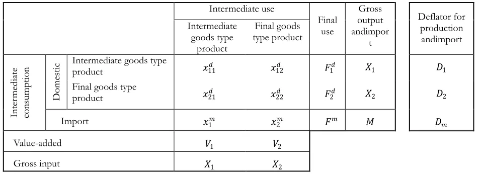
To include the influence on bias attributable to relative price change not only among domestic products but also between domestic products and imported goods, I introduce the input-output framework of an open economy as shown in Table 2.The framework is a non-competitive import category that separately records domestic products and imported goods. In this framework, for domestic products, the demand for gross output (𝑋) consists of intermediate use (𝑥𝑑) used in the production process and final use (𝐹𝑑) including consumption, investment, and export. Import
(𝑀) is also composed of intermediate use (𝑥𝑚) used in the production process and final use (𝐹𝑚) including
Table 2: Input-output framework of open economy and deflators (definition of variables) Intermediate use Final use Gross output andimpor t Deflator for production andimport Intermediate goods type product Final goods type product In ter me dia te co ns um pti on Do me st
ic Intermediate goods type product 𝑥11𝑑 𝑥12𝑑 𝐹1𝑑 𝑋1 𝐷1
Final goods type
product 𝑥21𝑑 𝑥22𝑑 𝐹2𝑑 𝑋2 𝐷2
Import 𝑥1𝑚 𝑥2𝑚 𝐹𝑚 𝑀 𝐷𝑚
Value-added 𝑉1 𝑉2
Gross input 𝑋1 𝑋2
Notes: Regarding the units of the variables, 𝐷1,𝐷2, and 𝐷𝑚 are deflators, and all others are values. 𝐷1isthe deflator for intermediate use (𝑥11𝑑 , 𝑥
12𝑑 ), final use (𝐹1𝑑), and gross output (𝑋1) of the intermediate goods type product;𝐷2 is
the deflator for intermediate use (𝑥21𝑑 ,𝑥
22𝑑 ), final use (𝐹2𝑑), and gross output (𝑋2) of the final goods typeproduct;
and𝐷𝑚is the deflator for the intermediate use of imported goods (𝑥1𝑚, 𝑥
2𝑚), the final use of imported goods (𝐹𝑚),
and import (𝑀).
Let us first consider nominal GDP as in the closed economy case previously described. Because GDP measured from the expenditure side (shown as 𝐹𝑈)is defined as “final use–import,” it is expressed by the following equation (10).
𝐹𝑈 = (𝐹1𝑑+ 𝐹
2𝑑+ 𝐹𝑚) − 𝑀 (10)
Substituting 𝑀 = 𝑥1𝑚 + 𝑥
2𝑚+ 𝐹𝑚 into equation (10), final use of import(𝐹𝑚)is canceled out and 𝐹𝑈 can
also be expressed in the following equation(11).
𝐹𝑈 = 𝐹1𝑑+ 𝐹2𝑑 − 𝑥1𝑚 + 𝑥2𝑚 (11)
Additionally, because “Final use of domestic products (𝐹𝑑)=Gross output–Intermediate use of domestic
products” from the supply-demand balance, substituting this into equation (11), the 𝐹𝑈 can be expressed further by the following equation (12).
𝐹𝑈 = 𝑋1− 𝑥11𝑑 + 𝑥12𝑑 + 𝑋2− 𝑥21𝑑 + 𝑥22𝑑 − (𝑥1𝑚 + 𝑥2𝑚) (12)
In contrast, because the added-value of each product is the difference between “Gross input” and “Intermediate consumption,” the production side GDP (expressed as 𝑉𝐴), which is the sum of added-value, is expressed by the following equation (13). It is self-evident that 𝑉𝐴 is equal to 𝐹𝑈 in equation (12).
𝑉𝐴 = 𝑉1+ 𝑉2= 𝑋1− 𝑥11𝑑 + 𝑥21𝑑 + 𝑥1𝑚 + 𝑋2− 𝑥12𝑑 + 𝑥22𝑑 + 𝑥2𝑚 (13)
Next, consider real GDP. Deflate each element of 𝐹𝑈 on the right side of equation (12), and real GDP measured from the expenditure side (shown as 𝐹𝑈 ) is represented by the following equation (13).
𝐹𝑈
=
𝑋1𝐷1
−
𝑥11𝑑𝐷1
+
𝑥12𝑑𝐷1
+
𝑋2 𝐷2−
𝑥21𝑑 𝐷2
+
𝑥22𝑑 𝐷2
−
𝑥1𝑚 𝐷𝑚
+
𝑥2𝑚
𝐷𝑚
(14)
The real GDP measured from the production side, required in the double-deflation method (shown as 𝑉𝐴 ), is defined as the difference between deflated “Gross input” and deflated “Intermediate consumption”and can be expressed as in equation (15).
𝑉𝐴 = 𝑋1
𝐷1
−
𝑥11𝑑𝐷1
+
𝑥21𝑑𝐷2
+
𝑥1𝑚 𝐷𝑚+
𝑋2 𝐷2
−
𝑥12𝑑 𝐷1
+
𝑥22𝑑 𝐷2
+
𝑥2𝑚
𝐷𝑚
(15) 𝑉𝐴
two-sided equivalence of real GDP (measured from the production side equal to the expenditure side) even in the open economy.
In contrast, the production side real GDP by single-deflation that deflates the nominal added-value of each product by an output deflator(shown as 𝑉𝐴) is expressed by the following equation (16). In this case, the real GDP equivalent cannot be guaranteed except when the relative price change between imported goods and each product is the same (𝐷1= 𝐷2= 𝐷𝑚).
𝑉𝐴
=
𝑉1 𝐷1+
𝑉2 𝐷2
=
𝑋1 𝐷1
−
𝑥11𝑑 𝐷1
+
𝑥21𝑑 𝐷1
+
𝑥1𝑚 𝐷1
+
𝑋2 𝐷2
−
𝑥12𝑑 𝐷2
+
𝑥22𝑑 𝐷2
+
𝑥2𝑚
𝐷2
(16)
Therefore, the bias, which is the difference between 𝑉𝐴 and𝑉𝐴 is as shown in the followingequation(17).The first item on the right side shows the effect on bias given the difference in the relative price change among domestic products, and the second and third items show the effect on bias given the difference in the relative price change between domestic products and intermediate import goods.
𝑏𝑖𝑎𝑠 = 𝑉𝐴
− 𝑉𝐴
=
𝑥12𝑑 −𝑥21𝑑 𝐷1−
𝑥12𝑑 −𝑥21𝑑 𝐷2
+
𝑥1𝑚 𝐷𝑚
−
𝑥1𝑚 𝐷1
+
𝑥2𝑚 𝐷𝑚
−
𝑥2𝑚
𝐷2
(17)
First item Second item Third item Effect on bias from Effect on bias from price change
Domestic product between domestic products and Relative price change intermediate imported goods
For the first item of equation (17) as the consideration from the closed economy input-output framework, because the single-deflation method generates a bias in the negative direction when the price increase of the intermediate good type product is larger than that of the final good type product (𝐷1> 𝐷2), the economic growth rate is underestimated. Conversely, if the price increases of the intermediate good type product is smaller than that of the final good type product (𝐷1< 𝐷2), because bias in the positive direction is generated, the economic growth rate is overrated. This conclusion is considered applicable not only in the case of two products but also in the case of a large number of products. That is, for the double-deflation method, the price increase of a domestic intermediate good decreases the real terms of the intermediate use (not intermediate consumption) of the product and increases the real added-value as an aggregate value (not of the product). In contrast, for the single-deflation method, correspondingly, the real term of intermediate use is overestimated and, thus, real GDP is underestimated. The reverse is also true. The magnitude of this effect is not uniform for all products but depends on the degree of intermediate good character or final good character of the product, the degree of deviation from the average price, and the size of the product in the economy. The greater the gross output, the greater the effect on GDP as an aggregate value. Industries in which the character of the product is neutral or whose price change equals the average price of all products do not bias real GDP as the aggregate value.
The second and third items on the right side of equation (17) indicate that bias occurs except when the price changes for the imported intermediate goods and each product are equal (𝐷𝑚 = 𝐷1, 𝐷2). In the single-deflation method, if the price increase of imported intermediate goods is larger than that of the domestic product (𝐷𝑚 > 𝐷1, 𝐷2), a bias in the negative direction is generated and the economic growth rate becomes underestimated. Conversely, for a price increase of the imported intermediate good that is smaller than that of the domestically produced (𝐷𝑚 < 𝐷1, 𝐷2), a bias in the positive direction is generated and the economic growth rate becomes overvalued.
3-2.Consideration using a numerical example
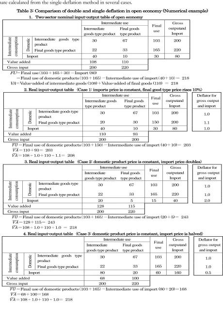
We confirm the conclusion from the open economy input-output framework using the numerical example of a two-sector table. Table 3 shows the relationship between real GDP using the double-deflation method and its estimate calculated from the single-deflation method in several cases.
Table 3: Comparison of double and single deflation in open economy (Numerical example)
1.Two-sector nominal input-output table of open economy
Intermediate use Final use Gross output and Import Intermediate
goods type product
Final goods type product In ter m ed iate co ns um ptio n D om es
tic Intermediate goods type product
30 67 103 200
Final goods type product 22 33 165 220
Import 40 10 30 80
Value added 108 110
Gross input 200 220
FU=Final use(103+165+30)-Import (80)
=Final use of domestic products(103+165)-Intermediate use of import(40+10)= 218
VA=Value-added of intermediate goods (108)+Value-added of final goods (110) = 218
2. Real input-output table〈Case 1: imports price is constant, final good type price rises 10%〉 Intermediate use Final use Gross output and Import Deflator for gross output and import Intermediate goods type product Final goods type product In ter m ed iate co ns um ptio n D om es
tic Intermediate goods type product
30 67 103 200 1.0
Final goods type product 20 30 150 200 1.1
Import 40 10 30 80 1.0
Value added 110 93
Gross input 200 200
𝐹𝑈
=Final use of domestic products(103+150)-Intermediate use of import (40+10)= 203 𝑉𝐴 =110+93= 203
𝑉𝐴=108 ÷ 1.0+110 ÷ 1.1= 208
3. Real input-output table〈Case 2: domestic product price is constant, import price doubles〉 Intermediate use Final use Gross output and Import Deflator for gross output and import Intermediate
goods type product
Final goods type product In ter m ed iate co ns um ptio n D om es
tic Intermediate goods type product
30 67 103 200 1.0
Final goods type product 22 33 165 220 1.0
Import 20 5 15 40 2.0
Value added 128 115
Gross input 200 220
𝐹𝑈
=Final use of domestic products(103+165)-Intermediate use of import (20+5)= 243 𝑉𝐴 =128+115= 243
𝑉𝐴=108 ÷ 1.0+110 ÷ 1.0 = 218
4. Real input-output table〈Case 3: domestic product price is constant, import price is halved〉 Intermediate use Final use Gross output and Import Deflator for gross output and import Intermediate
goods type product
Final goods type product In ter m ed iate co ns um ptio n D om es
tic Intermediate goods type product
30 67 103 200 1.0
Final goods type product 22 33 165 220 1.0
Import 80 20 60 160 0.5
Value added 68 100
Gross input 200 220
𝐹𝑈
=Final use of domestic products(103+165)-Intermediate use of import (80+20)=168 𝑉𝐴 =68+100=168
First, we confirm the two-sided equivalence of nominal GDP using a numerical example. In “1. Two-sector Nominal Input-output Table of Open-economy” in Table 3, the expenditure side of nominal GDP (shown as 𝐹𝑈, in this case 218) is defined as the difference between “Final use (in this case, 103 + 165 + 30 = 298)” and “Import (in this case 80)” or the difference between “Final use of domestic products (in this case, 103 + 165 = 268)” and “Intermediate use of import (in this case, 40 + 10 = 50)” and equals the production side nominal GDP (shown as 𝑉𝐴, in this case, also 108 + 110 = 218).
Next, we consider real GDP in several cases.
First, how does the relative price change among domestic products affect single-deflation bias? As one of the main conclusions from the empirical analysis targeting Japan during 1960–2000 by Li and Kuroko (2016), the primary industry and many secondary industries have significant characteristics of intermediate goods, and many tertiary industries have strong characteristics of final goods. As a trend, with economic growth, the product prices in the primary industry and the secondary industry will decrease relatively, and prices in the tertiary industry will increase relatively given the increase in the price of labor. Therefore, the price of the product of the intermediate goods character relatively decreases, and the price of the product of the final good character relatively increases.
Using this conclusion, I develop Case 1 as shown in “2.Real Input-Output Table” in Table 3, a numerical example in which the price of the product of the final good character increases relatively (D2>D1). In this case, the assumption is that the price of imported goods does not change, and the price of the final good type product increases by just 10%. That is, gross output and each use item of intermediate good type products are deflated by 1.0, those of the final good type product are deflated by 1.1, and imports are deflated by 1.0. For each product, the deflated “Intermediate consumption “of domestic production and imports is subtracted from the deflated “Gross input = Gross output,” then real added-value by the double-deflation method(shown as 𝑉𝐴 , in this case,110 + 93=203) is calculated. This situation is equivalent to real GDPexpenditures (shown as𝐹𝑈 , in this case,203), which is the difference between the deflated “Final use” of domestic products (103 + 150=253) and the “Intermediate use” of imports (40 + 10=50).In contrast, the estimated real value-added by the single-deflation method that deflates the added-value of each product directly using the output deflators 1.0 and 1.1 can also be obtained (108 + 100). In this case, because the second item of the right side of equation (17) is zero, and the first and third items are positive values, the estimated real GDP by the single-deflation method (shown as 𝑉𝐴, in this case,108 + 100 = 208)is slightly larger than the production side real GDP by the double-deflation method (shown as 𝑉𝐴 =𝐹𝑈 = 203).
Next, we examine how price changes of imported intermediate goods influence the bias. In the case of Japan, mineral fuels such as petroleum are representative imported intermediate goods. Empirical analysis by Li and Kuroko (2016) showed that, as an overall trend of Japan during the 1960–2000 periods, final goods prices increased relative to those of intermediate goods, and the estimated production side real GDP by the single-deflation method was overestimated but undervalued only in the two oil shock periods. The oil price increased more than three times during the first oil shock in 1978 and increased by 70% during the second oil shock in1980. Normally, the changes in world market prices, such as for petroleum, and exchange rates are much larger than such changes in domestic products.
Finally, we observe cases of the currency appreciation or price decreases of imported intermediate goods, such as oil price declines.“4. Real Input-Output Table” in Table 3 shows Case 3,in which the import price is halved, and no price change occurs between domestic products. In this case, the gross output and each use item of domestic products of intermediate and final good types are deflated by 1.0, and “Intermediate use” and “Final use” of imports are deflated by 0.5. Additionally, the deflated “Intermediate consumption” is subtracted from the deflated “Gross output “and real added-value by the double-deflation method (shown as 𝑉𝐴 , in this case,68 + 100 = 168), is required. This value is equivalent to real GDP expenditures (shown as 𝐹𝑈 , in this case,168), which is the difference between the deflated “Final use” of domestic products (103 + 165 = 268) and the “Intermediate use” of imports (80 + 20 = 100). For the same reason as in Case 2, the estimated real GDP by the single-deflation method (shown as 𝑉𝐴, in this case, 108÷1.0 + 110÷1.0 = 218) remains the nominal added-value. In this case, because the first item of equation (17) is zero and the second and third items are positive values, the estimated real GDP by the single-deflation method (shown as 𝑉𝐴 = 218) is considerably larger than the production side real GDP by the double-deflation method (shown as 𝑉𝐴 = 𝐹𝑈 = 168).
4.Empirical analysis using JSNA data
Alexander et al. (2017) used data since 2000 for the eight G20 countries (Belgium, Brazil, Canada, France, Japan, Korea, the Netherlands, and the United States) that use the double-deflation method, to calculate the constant price values that would have pertained if those countries had utilized the single-deflation method and compared the results with the official estimate of the double-deflation method. The mean difference for the entire period (annual basis is unpublished) indicated that five countries (Belgium, France, Japan, the Netherlands, the United States) underestimate and three countries (Brazil, Canada, South Korea) overestimate. The mean absolute difference shows that Japan, Korea, and Brazil have the largest impact from single deflation and the influence on EU member countries is relatively small.
In this section, following the same method, I use JSNA data for 1955–2017 to calculate the realGDP growth rate that would have pertained if Japan had utilized the single-deflation method and compare the result with the official estimate from the double-deflation method. Furthermore, I analyze the cause of the bias using the considered results from the open economic input-output framework presented in the previous section.
4-1.Creation of input–output tables and SNA in Japan
Before using the data to conduct the analysis, I briefly introduce related government statistics from Japan. The creation of government statistics in Japan is a decentralized mechanism through which each ministry prepares its statistics according to its administrative tasks. For this reason, the input-output table and SNA statistics are also made by different ministries.
First, the history of preparing input-output tables in Japan is long. The practice began in 1951 when each ministry created an individual table. After the 1955 table, every five years, table creation was a joint project of the concerned ministries. Today, together with the Ministry of Internal Affairs and Communications statistics bureau as a collector, the relevant 10 ministries including the Cabinet Office jointly create the table. Basically, it creates for the year whose tail is 0 or 5.6The first purpose of these tables is to analyze the economic ripple effect by factorizing the table, and the second purpose is to use it as a benchmark of JSNA statistics. For the purpose of the former, the definition of each item of the output table does not necessarily completely match with SNA. In addition, after the input-output table is created, the lined constant price input-input-output table, which has comparability with the tables created up to that time every five years, is created. Using this lined input-output table, Li and Kuroko (2016) compared the GDP growth rate of the double and single-deflation methods for Japan during 1960–2000.
In contrast, JSNA as processing statistics is prepared by the Economic and Social Research Institute (ESRI), Cabinet Office. Every five years, JSNA annually revises the standard as a benchmark for estimating GDP after the completion of the input-output tables. That is, the benchmark year of JSNA is the year of the input-output table. From the 2000 benchmark year, the chain-linked method was introduced with real terms and was published in parallel with those of the conventional constant price method. Since the 2011 benchmark year, the constant price method has been abolished, and only the real terms from the chain-linked method have been made public.
4-2.Measurement of Japan 1994–2017
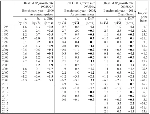
ESRI moved JSNA to the 1993 SNA in 2000 and the 2008 SNA in 2016.Both series are retrospectively estimated until 1994.In the “National Accounts Annual Report” by ESRI, the nominal and real terms of the GDP and the output deflator classified by economic activity are published. I use these data to calculate the GDP growth rate when using the single-deflation method (𝑉𝐴) from1995 to 2017in Japan. First, the nominal GDP classified by economic activity is deflated with the output deflator, and the GDP growth rate is calculated by aggregating the deflated GDP classified by economic activity. Table 4 shows a comparison between the calculation result and the official GDP growth rate estimate using the double-deflation method (𝑉𝐴 ).
Table 4: Japan 1995–2017 comparison between single-deflation and official GDP growth rate estimate(percentage points)
Real GDP growth rate. 1993SNA, Benchmark year = 2000,
At constantprices
Real GDP growth rate. 1993SNA, Benchmark year =2005,
At constant prices
Real GDP growth rate. 2008SNA, Benchmark year = 2011,
Chain-linked
d. Import price index a.
by 𝑉𝐴
b. by𝑉𝐴
c. Diff. (b-a)
a. by 𝑉𝐴
b. by𝑉𝐴
c. Diff. (b-a)
a. by 𝑉𝐴
b. by𝑉𝐴
c. Diff. (b-a)
1995 1.6 1.3 −0.2 0.7 0.8 0.1 1.8 1.9 0.1 1.0
1996 2.8 2.4 −0.3 2.7 2.0 −0.7 2.7 2.5 −0.1 28.0
1997 1.2 0.7 −0.5 1.7 0.9 −0.8 1.0 0.8 −0.2 15.0
1998 −1.7 −1.0 0.8 −1.8 −1.0 0.7 −1.3 −0.5 0.9 −21.0
1999 0.1 0.2 0.1 0.4 0.4 0.0 −0.2 0.1 0.3 −3.0
2000 2.2 1.3 −0.9 2.0 0.9 −1.1 1.9 1.1 −0.8 41.2
2001 −0.5 −0.5 −0.1 −0.8 −1.1 −0.2 −0.1 −0.5 −0.4 6.6
2002 0.6 0.6 −0.1 0.3 0.0 −0.4 0.1 0.0 −0.1 −1.9
2003 2.0 1.2 −0.8 1.1 0.5 −0.6 0.9 0.5 −0.4 6.7
2004 2.7 1.4 −1.3 2.1 1.0 −1.1 1.6 0.8 −0.8 11.2
2005 3.1 1.2 −1.9 1.7 0.2 −1.6 1.8 0.4 −1.4 38.7
2006 1.8 0.1 −1.7 1.9 0.2 −1.7 1.1 −0.4 −1.6 26.5
2007 2.7 1.0 −1.7 2.2 1.0 −1.2 1.3 0.3 −1.0 8.4
2008 −1.2 −3.6 −2.5 −1.2 −3.5 −2.2 −1.2 −3.4 −2.2 34.3
2009 −7.3 −4.2 3.1 −6.2 −3.1 3.1 −6.0 −2.8 3.2 −40.8
2010 4.9 3.6 −1.3 3.5 3.0 −0.6 16.9
2011 −0.3 −1.8 −1.5 −0.3 −1.9 −1.6 25.4
2012 1.0 1.3 0.4 1.3 1.5 0.2 6.0
2013 0.8 0.2 −0.7 2.0 1.1 −0.9 16.6
2014 0.6 −0.1 −0.7 0.4 −0.2 −0.5 3.6
2015 1.4 3.5 2.2 −34.0
2016 0.4 2.5 2.1 −31.4
2017 2.0 0.5 −1.4 33.9
Source: Economic and Social Research Institute, Cabinet Office, Government of Japan. Notes:
a. This GDP growth rate is calculated by the aggregate published “Gross Domestic Product Classified by Economic Activities in Real Terms,” which is estimated by the double-deflation method. However, for “Benchmark year = 2000” and “Benchmark year = 2005,” the constant price method was adopted in which additive consistency was established.
b. This GDP growth rate is calculated as the real terms aggregated from “Gross Domestic Product Classified by Economic Activities at Current Prices” directly deflated by its output deflator.
c. Difference in GDP real growth ratio (%) = a. GDP growth rate by 𝑉𝐴 – b.GDP growth rate by 𝑉𝐴
Additionally, to analyze the bias using the results of consideration from the open economy input-output framework, Table 4 shows the import price increase rate for mineral fuels, such as crude oil, which is a representative import intermediate good in Japan. Because this indicator is Japan’s import price index, it reflects both factors the currency and the price change of the good in the international market.
We first observe the GDP growth rate of the official statistics estimated by the double-deflation method (a.by
𝑉𝐴
) as shown in Table 4. Nevertheless, the series is based on the same 1993SNA because the benchmark input-output
table used for the estimation differs between 2000 and 2005, and the annual GDP growth rates are different among those series. After shifting to the latest 2008 SNA international standard, the annual growth rate is more different from the previous benchmark year data. Of course, the GDP growth rates calculated by the single-deflation method (b.by 𝑉𝐴) using the added-value estimate from the three benchmark’s input-output table are also different.
Moreover, the sizes of the difference (c.Diff.(b-a)) in the GDP growth rate calculated by the two estimation methods also differ considerably given the difference in the benchmark year. However, paying attention to the direction (+ or –) of the difference, that is, the direction of the single-deflation bias, they are almost the same. In particular, the significant bias in the negative direction is observed after 2000.In other words, during this period, the real added-value estimated by the single-deflation method underestimates the real GDP.As an exception, only 1998, 2009, 2015, and 2016 showed a very large positive bias, especially in 2009.7
A comparison of the direction of bias with the import price increase rate of mineral fuels including crude oil markedly shows that, for most years, the significant increases in the import intermediate goods price generate a minus direction bias, whereas forall of the years during which import intermediate goods prices significantly declined, a plus direction bias was generated. This result is consistent with that of consideration of the relationship between the relative price change of imported and domestic products used for intermediate consumption and the direction of the bias shown in the second and third items of equation (17).The relative price change between Japanese domestic products during that period is considered not large, and the influence of the first item is not significant.
In the comparative analysis of the eight countries that adopt the double-deflation method by Alexander et al. (2017),the underestimation (bias in the negative direction) is the mean of the difference between the single-deflation method, and the official GDP growth rate estimates are from five countries including Japan, whose mean is the largest negative value.8 The same content was reported at the OECD Joint Meetings of the Working Parties on Financial Statistics and National Accounts (WPNA) held in October 2016.9At that time, since the 2011 benchmark revision in Japan was not completed yet, the comparison by Alexander et al. (2017) is based on the “1993 SNA, Benchmark year=2005”data in Table 4.Its conclusion is also consistent with the estimation results in Table 4.
4-3.Measurement of Japan 1956–1998 conforming to 1968 SNA
Japan introduced 1968 SNA in 1978 and started the double-deflation method to realize added-value. Recently, ESRI published retrospective estimate data up to 1955. This“ Long-term retrospective major series of national accounts report (1968SNA, Benchmark year = 1990)”includes the published nominal and real terms of GDP and gross output classified by economic activity. I use these data to calculate the GDP growth rate when using the single-deflation method from1956 to 1998 Japan. For the calculation, first, the output deflator from the nominal and the real terms of gross output classified by economic activity is calculated, and the nominal GDP classified by economic activity is deflated by the deflators. Finally, the GDP growth rate using the same procedure as in the previous section (b.by 𝑉𝐴) is calculated and is compared with the official GDP growth rate estimate, which is using by the double-deflation method (a. by 𝑉𝐴 ).
7Alexander et al.(2017)also pointed out that it was in 2009. 8See Alexander et al.(2017), p.12.
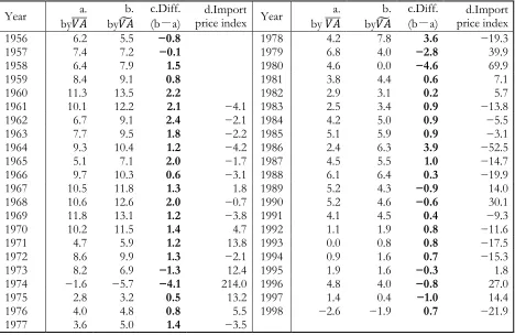
Table 5: Japan 1956–1998 comparison between single-deflation and official GDP growth rate estimate (percentage points)(1968SNA, Benchmark year = 1990,At Constant Prices)
Year by𝑉𝐴 a. by𝑉𝐴b. c.Diff. (b-a) price index Year d.Import by 𝑉𝐴 a. by𝑉𝐴b. c.Diff. (b-a) price index d.Import
1956 6.2 5.5 −0.8 1978 4.2 7.8 3.6 −19.3
1957 7.4 7.2 −0.1 1979 6.8 4.0 −2.8 39.9
1958 6.4 7.9 1.5 1980 4.6 0.0 −4.6 69.9
1959 8.4 9.1 0.8 1981 3.8 4.4 0.6 7.1
1960 11.3 13.5 2.2 1982 2.9 3.1 0.2 5.7
1961 10.1 12.2 2.1 −4.1 1983 2.5 3.4 0.9 −13.8
1962 6.7 9.1 2.4 −2.1 1984 4.2 5.0 0.9 −5.5
1963 7.7 9.5 1.8 −2.2 1985 5.1 5.9 0.9 −3.1
1964 9.3 10.4 1.2 −4.2 1986 2.4 6.3 3.9 −52.5
1965 5.1 7.1 2.0 −1.7 1987 4.5 5.5 1.0 −14.7
1966 9.7 10.3 0.6 −3.1 1988 6.1 6.4 0.3 −19.9
1967 10.5 11.8 1.3 1.8 1989 5.2 4.3 −0.9 14.0
1968 10.6 12.6 2.0 −0.7 1990 5.2 4.6 −0.6 30.1
1969 11.8 13.1 1.2 −3.8 1991 4.1 4.5 0.4 −9.3
1970 10.2 11.5 1.4 4.7 1992 1.1 1.9 0.8 −11.6
1971 4.7 5.9 1.2 13.8 1993 0.0 0.8 0.8 −17.5
1972 8.6 9.9 1.3 −2.1 1994 0.9 1.6 0.7 −15.3
1973 8.2 6.9 −1.3 12.4 1995 1.9 1.6 −0.3 1.8
1974 −1.6 −5.7 −4.1 214.0 1996 4.8 4.0 −0.8 27.0
1975 2.8 3.2 0.5 13.2 1997 1.4 0.4 −1.0 14.4
1976 4.0 4.8 0.8 5.5 1998 −2.6 −1.9 0.7 −21.9
1977 3.6 5.0 1.4 −3.5
Source: Economic and Social Research Institute, Cabinet Office, Government of Japan“Long-term retrospective major series of national accounts report (1968SNA, Benchmark year = 1990).”
Notes:
a.This GDP growth rate is calculated by the aggregate published “Gross Domestic Product Classified by Economic Activities (At Constant Prices),” which is estimated by the double-deflation method.
b.This GDP growth rate is calculated as the aggregate real terms, such that “Gross Domestic Product Classified by Economic Activities (At Current Prices)” is directly deflated by its output deflator. Because the output deflator of the published figures is rounded off to one decimal place, here it is calculated by using the nominal terms of gross output classified by economic activities ÷ the real terms.
c.The differences in GDP real growth ratio (%) =a. GDP growth rate by 𝑉𝐴 – b. GDP growth rate by 𝑉𝐴
d. The import price change indicator here is the price increase rate of mineral fuels including crude oil. Source: Japan Tariff Association. Ministry of Finance. “Mineral fuels”
They pointed out that the price of services, which are final goods type products, increased relative to that of intermediate goods type products because the price of labor in Japan increased sharply during this period. In other words, the relative price change between domestic products is large during the period; therefore, the influence of the first item of equation (17) is considered to be large.
5. Conclusion
In this paper, using the open economy input-output framework, I clarified the relationship between the relative price change, including among domestic products and between domestic products and imported goods, and the single-deflation bias for the first time in mathematical formulas. Specifically, if the price increase of domestic intermediate good type products is larger than that of the final good type product, the single-deflation method generates a bias in the negative direction and underestimates the GDP growth rate. In contrast, if the price increase of the domestic final good type product is larger than that of the intermediate good type product, a bias in the positive direction is generated, and the GDP growth rate is overrated. Moreover, if the price increase of import intermediate goods is larger than that of domestic products, a bias in the negative direction is generated, and the GDP growth rate is underestimated. Moreover, if the price of the import intermediate good declines relatively, a bias in the positive direction is generated, and the GDP growth rate is overrated. I also explained the mechanism using numerical examples of the open economy input-output table.
I also calculated the single-deflation bias for each year from 1956 to 2017using JSNA data and compared it with fluctuations in import prices of mineral fuels, including crude oil, which is a representative import intermediate good in Japan. The comparison confirmed that, in the case of Japan, the direction of the bias is closely related to the price fluctuation of imported intermediate goods.
The bias direction was also observed to have different characteristics depending on the time. To observe more clearly the features of each period, Table 6 shows the mean of the differences every five years as calculated from Table 4 and Table 5. From here, the bias in the positive direction (excluding the oil shock period) is frequently and overwhelmingly observed during the period from 1960 to the early 1990s. In contrast, the bias in the negative direction is observed much more after 2000. Generally, as the economy grows, the price increase of services will be greater than that of goods. In the past, services had strong characteristics as final goods because the service for enterprises increased and the intermediate consumption of the service industry increased after 2000. The fact that the service industry has strengthened its character as an intermediate good might be one cause. Accumulating more empirical analysis, including factorization, on this issue is necessary.
Table 6: Mean of the difference between single-deflation and official GDP growth rate estimate
Sample Period
1968SNA 1993SNA 1993SNA 2008SNA Benchmark year =
1990 2000 2005 2011
1960–1964 1.92
1965–1969 1.43
1970–1974 −0.32
1975–1979 0.70
1980–1984 −0.42
1985–1989 1.04
1990–1994 0.43
1995–1999 −0.02 −0.14 0.16
2000–2004 −0.64 −0.68 −0.49
2005–2009 −0.94 −0.72 −0.58
2010–2014 −0.76 −0.69
2015–2017 0.94
Source: Calculated from Table 4 and Table 5.
Acknowledgements: In preparing this paper I would like to thank Mr. Masato Kuruko (Institute of Developing
References
Alexander, Thomas, Claudia Dziobek, Marco Marini, Eric Metreau and Michael Stanger (2017) “Measure up: A Better Way to Calculate GDP” IMF Staff Discussion Note, SDN/17/02. [Online] Available:
https://www.imf.org/~/media/Files/Publications/SDN/2017/sdn1702.ashx
Bean, Charles (2016) Independent review of UK economic statistics: final report, March.[Online] Available: https://www.gov.uk/government/uploads/system/uploads/attachment_data/file/507081/2904936_Bean_R eview_Web_Accessible.pdf
Claudia Dziobek (2016) “GDP- Lost in Single Deflation” OECD Joint Meetings of the Working Parties on Financial Statistics (WPFS) and National Accounts (WPNA), Paris, October 27, 2016. [Online] Available: http://www.oecd.org/officialdocuments/publicdisplaydocumentpdf/?cote=STD/CSSP/WPNA(2016)20&d ocLanguage=En ]
Nicholas Oulton, Ana Rincon-Aznar, Lea Samek, Sylaja Srinivasan (2018) “Double deflation: Theory and Practice”. [Online] Available: http://www.iariw.org/copenhagen/oulton.pdf]
Li, Jie and Masato Kuroko (2016) “Single Deflation Bias in Value Added: Verification Using Japanese Real Input-Output Tables (1960–2000)” Journal of Economics and Development Studies, Vol. 4, No. 1.
Li, Jie (2016) China’s GDP statistics – Comparison with Japan: Estimation Methods and Relevant Statistics, Saarbrücken, Germany: Scholars' Press.
Li, Jie (2017) “Is China's GDP Growth Overstated? An Empirical Analysis of the Bias Caused by the Single Deflation Method” Journal of Economics and Development Studies, Vol. 5, No. 4.