Forestry & Natural-Resource Sciences Last Correction: Apr. 18, 2011
KRIGING WITH EXTERNAL DRIFT IN MODEL LOCALIZATION
Minna R¨
aty
1,
Juha Heikkinen
2,
Annika Kangas
31Ph.D. Student,3Prof., Department of Forest Science, University of Helsinki, Finland.3Ph.:+358 9 191 58 177
2Senior Researcher, The Finnish Forest Research Institute, PL 18, FI-01301 Vantaa, Finland, Ph.:+358 10 211 5420
Abstract.When modelling a large area, models that can take into a count the variation from the general
mean in small sub-areas could perform better in prediction than a general model fitted to entire dataset. One method for adjusting the large-area models for such variation is kriging, in which the predictions are corrected with the aid of neighbouring observations. A variogram represents the spatial correlation between neighbouring observations as a function of distance. The predictions are obtained using a drift model that describes the general mean, and the selected variogram. The aim of this study was (1) to test for a spatial correlation in the residuals of a global form height model fitted over a large study area and (2) to use this correlation in prediction of the same variable. The dataset consisted of measurements from 19 175 Scots pines (Pinus sylvestris L.) from the 9th National Forest Inventory of Finland. Nested spherical and Bessel variograms were selected for the kriging calculations. In nested models the short-range (intra-stand) correlation and long-range (inter-stand) correlation are modelled separately. We used cross-validation to evaluate the variogram models selected. At the global level, 30 neighbours were needed for stable estimates, and with 60 neighbours the root mean squared prediction errors (RMSPE) of kriging were lower than those of the global model. At the regional level, we obtained better estimates than with regionally re-fitted models when the number of neighbours was 60 for both variogram models. The mean biases (i.e., average difference between actual and predicted values) at the regional level in the kriging predictions were small (0.8% of the regional RMSPE). In conclusion, there was an app. 6-km spatial correlation in the residuals, but due to relay effect the size of the kriging neighbourhood required for improving prediction was larger than the range.
Keywords:KED, Kriging, Localization, Regression, Semivariance, Variogram
1
Introduction
Forest inventory is based on samples that are used to estimate the values of interest in the entire population (e.g. Shiver and Borders, 1996; Johnson, 2000). For instance, for all measured trees (the tally trees), often only basic characteristics such as species and diameter at breast height (usually, 1.3 m above ground; DBH) are measured. Only a proportion of them (sample trees) are measured for height and other characteristics. Models describing the variables measured from sample trees as a function of variables measured from tally trees are used to generalize these variables to tally trees. Commonly in forest inventories, the species and DBH are obtained for all trees of a plot, and for a subset of these trees, height and other measures are taken. A global regres-sion model (i.e. model covering the entire study area) is a tempting alternative in such situations because it is easy to implement once it has been formulated. The problems in such models occur before implementation;
i.e.in finding the correct form of dependences between the dependent and independent variables.
When the dependences are found, the model needs to be validated. One requirement for a global model is that the model is not biased with respect to any inde-pendent variable, i.e. residuals do not have any trends over space, but are instead randomly distributed over space. If this requirement is fulfilled, questions still re-main: “How well will this global model predicted for smaller regions? Will there be a trend of residuals over space?” One alternative to the global model is to use local models. The definition of a local model is ambigu-ous. In predicting at a local area, the options include: 1) fitting the global model for each region; 2) including region as a class variable in the model, along with in-teractions with all continuous variables, resulting in the same coefficients as with option 1) but fitting is based on the entire data set resulting in increased precision; or 3) fitting a regional specific model with different explana-tory variables. Of these options, option 2 makes use of
the entire dataset, resulting in the same coefficients as option 1), but with lower standard errors of coefficients. Another problem is to define the optimal regions for the localization, since localization based on administra-tive borders, such as forestry centres in Finland, is not necessarily the most accurate. In defining the localiza-tion areas, three issues need to be considered. First and most important, the regions should be as homogeneous as possible with respect to the global regression residu-als. The smaller the regions are, the more homogeneous they also can be. Second, the optimal sizes of the sub-areas delineated must be defined. Most probably there is some threshold size for the sub-area below which the lo-calizing does not improve the predictions significantly or the result may even be poorer than before localization. The size and number of sub-areas are related, even if the sub-areas are not evenly sized. Third, it needs to be considered if there is any practical reason to constraint the shapes of the regions.
As an alternative to including local region as a fixed effect class variable in a global model, or fitting separate local models, spatial prediction approaches offer alterna-tives. These spatial prediction approaches can be use to localize the model without strict spatial (i.e., regional) boundaries, using all neighbourhood. The concept of spatial association (SA) (e.g. Cliff and Ord, 1981) sim-ply states that two observations near each other are most probably more alike than two observations that are far-ther apart. One way to test the existence of SA is to cal-culate spatial indicators, e.g. I-, C-, G-, and G*-indices, both local and global (Anselin, 1995; Getis and Ord, 1992; 1996; Boots, 2002). The other way to find the SA, although in continuous form, is to calculate a spatial cor-relation from the data. If this spatial corcor-relation from the neighbourhood of an observation is utilized in pre-dictions, in connection with the global regression model, the method is called universal kriging, kriging with ex-ternal drift (KED), kriging with distinction, or residual kriging (Hengl et al., 2003; Schabenberger and Gotway, 2005). In this paper, we will use the terms universal kriging and KED. In kriging the spatial correlation is modelled with a distance and direction dependent var-iogram. Typically, the correlation is strongest near the origin and vanishes within finite range.
The origins of kriging are in minefield calculation and geology (e.g. Isaaks and Srivastava, 1989). Since then, the method has spread widely to other disciplines, such as remote sensing and ecological surveying in seed zone and biomass mapping (Hamann et al., 2000; Sales et al., 2007); interpolation of parameters (Nanos and Montero, 2002); temporal and multi-resolution studies (Fuentes et al., 2006; Johannesson et al., 2007; Magnussen et al., 2007); studies in combination with mixed models (Nanos et al., 2004), and prediction of leaf litterfall (Staelens
et al., 2004). One of the most common applications of kriging is the interpolation of point or plot data onto a surface using geographic information system (GIS) soft-ware.
In universal kriging, the prediction given by regres-sion model is ‘corrected’ or ‘adjusted’ to fit the sur-rounding observations of residuals. The residuals are weighted with the variogram model presenting the SA in the neighbourhood (Webster and Oliver, 2007). In the present study, the regression model is a tree level form height model that is fitted over the study area. The correlation of the residuals of the global model, i.e. the SA, is studied. Actually, to be precise, we used var-iograms and variances instead of the correlation; these two are optional and one can be converted to the other. Finally, we calculated the kriging predictions of form height for all the trees with the given variogram and regression model. Our purpose was to compare these re-sults from the universal kriging with previous regression model localization results, in which our focus in addi-tion to localizaaddi-tion was on the various methods used to divide the study area into homogeneous regions (R¨aty and Kangas, 2008; 2010).
2
Materials and methods
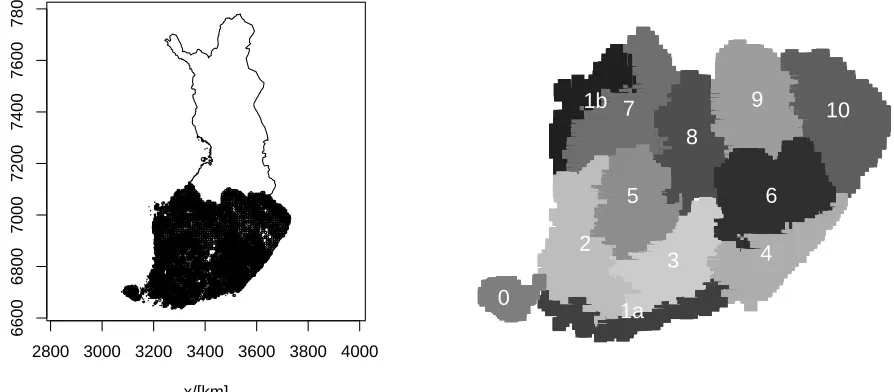
2.1 Study area description and sampling The study area was located in Southern Finland (Fig. 1). It covered all the forest land both private and state forests, managed and unmanaged forests. The study area belonged to boreal zone and forests were mixed forests where the dominant species are Scots pine (
Pi-nus sylvestris L.), Norway spruce (Picea abies L.) and Silver Birch (Betula pendula L.). Data from the 9th National Forest Inventory (NFI) collected from 1996 to 2003 (not repeated measures data) were used for this study. The NFI was systematic cluster sampling, where plots were arranged in clusters and trees were measured from these angle gauge plots (also called variable radius or unequal probability sample plots) using a basal area factor (BAF) of 2 m2/ha. There were three different
regions in respect to the sampling design in the study area. Because the sampling design varied (for example, the number of plots was from 10 to 18 depending on the region), we have collected some statistics about the inter-plot, intra-cluster and inter-cluster distances (Ta-ble 1; NFI9, 2011).
2800 3000 3200 3400 3600 3800 4000
6600
6800
7000
7200
7400
7600
7800
x/[km]
y/[km]
0
1a
2
3
4
5
6
7
8
9
10
1b
Figure 1: Left - Study area in southern Finland. Right - forestry centres within the study area.
Table 1: Statistics for distances (km) to describe the sampling design in different regions in study area.
Region Forestry Inter-plot Intra-cluster Inter-cluster Inter-cluster
centres minimum maximum minimum plot minimum
˚
Aland 0 0.25 2.5/1.8 4.2/6 1.5
Southernmost Finland 1a, 2, 3, 4, 5, 6 0.25 2.5/1.8 6 4.5
Central Finland 1b, 7, 8, 9, 10 0.30 2 7 5.5
one sample tree at plot, the maximum was five trees.
We calculated minimum, median, mean and maximum distances to the nearest neighbouring sample trees for each forestry centre and for varying number of bours (Table 3). For 40 neighbours the smallest neigh-bourhood was a 5.8-km circle in forestry centre 0, while the overall average was 10.7 km and the maximum 40.9 km in forestry centre 1b. For 60 and 100 neighbours the average distances were 13.4 km and 17.4 km, re-spectively. Forestry centres 1a and 1b on the south and north coasts of the study area had the largest distances, since there were plot clusters on islands in those parts of the area and relatively sparse sampling design. The distances were also large in forestry centre 3, probably due to the low number of total observations compared with the size of the area (Fig. 1b; Table 7). The ˚Aland, forestry centre 0, had the smallest neighbourhoods, but also the densest sampling design. Inner forestry centres (5 and 6) also had distances among the shortest of any of their neighbours. Since the kriging calculations were not limited to these administrative regions, neither were the neighbourhoods above. Trees near the border may have neighbours from other forestry centres as well. The neighbourhood is always the given number of nearest
ob-servations regardless of the location in forestry centre. This is different from the previously used methods where only the observations within selected sub-area are used in localization (R¨aty and Kangas, 2006; 2008; 2010).
2.2 Global model We fitted the global form-height model using diameter at breast height, basal area, and distance to the coast, as well as a quadratic surface using spatial coordinates as explanatory variables as follows:
v
d2 =β0+β1d+β2d2+β3ln (G) +
+α1XC+α2XC2+α
3XC·Y C+
α4Y C+α5Y C2+α6RDIST +ε,
(1)
where dv2is a measure proportional to the form height of a tree, which we will later simply refer to as form height;
dis DBH;Gis total basal area of the plot including all tree species; andεis the residual error at the tree level. The XC and XY coordinates and RDIST were scaled using the following: the scaled spatial variables XC, YC and RDIST (Eq. 2):
⎧ ⎪ ⎪ ⎨ ⎪ ⎪ ⎩
Y C= Y−10006620
XC = X−60
1000
RDIST = 1
DIST+0.05, DIST ≤20
RDIST = 0, , DIST >20
,
Table 2: Statistics for Scots pine (Pinus sylvestris) sample trees: diameter at breast height, diameter at 6 m height, height, volume,v/d2(measure proportional to form height) and actual form height in the study data. G is the total basal area of the corresponding sample plots.
Min. 1stQ Med. Mean 3rdQ Max.
d [cm] 5 14 19 20.55 27 67
d6[cm] * 11 16 16.4 22 51
h [dm] 20 105 146 150 193 352
v [dm3] 3.7 80 204 331 479 2882
G[m2/ha] 1 16 21 21.15 27 60
v/d2 [dm3/cm2] 0.148 0.413 0.543 0.553 0.677 1.305
fm [m] 1.9 5.3 6.9 7 8.6 16.6
∗2561 of the sample trees were less than 6 m in height.
Table 3: Distances (km) to the 40, 60 and 100 closest neighbours by the forestry centre (FC).
FC Minimum Median Mean Maximum
Neighbours 40 60 100 40 60 100 40 60 100 40 60 100
0 5.8 8.3 11.0 8.7 10.5 15.2 9.9 12.4 17.0 25.2 28.5 35.0
1a 7.0 9.1 13.2 12.5 15.1 20.2 12.5 16.3 20.8 31.8 36.9 44.0
1b 7.4 9.4 14.1 11.0 14.5 19.4 12.3 14.9 19.8 40.9 44.3 50.7
2 6.4 8.0 12.0 9.3 12.4 16.5 10.0 12.6 16.3 25.0 27.7 32.6
3 7.3 9.0 12.8 12.8 14.9 19.8 12.6 15.7 20.2 19.2 25.1 29.3
4 6.0 7.4 12.0 9.1 12.2 14.3 10.0 12.6 16.1 30.4 32.7 36.6
5 6.0 7.8 11.0 9.6 12.5 16.5 10.2 12.7 16.5 18.0 21.4 25.3
6 6.6 8.5 12.4 9.2 12.4 16.1 9.8 12.5 15.9 15.4 19.8 24.1
7 7.0 8.9 13.6 9.7 13.2 15.5 10.3 12.9 16.7 16.8 21.0 27.7
8 7.0 8.2 11.0 9.9 13.7 16.2 10.9 13.4 17.7 21.0 23.6 29.3
9 7.0 9.3 14.0 12.5 15.5 19.8 12.2 14.5 19.5 19.6 22.4 28.3
10 7.0 8.2 12.5 9.7 13.7 15.8 10.6 13.4 17.7 23.5 28.4 34.5
where X and Y are the spatial positions in Kartastoko-ordinaattij¨arjestelm¨a (KKJ), which is a national Gauss-Kr¨uger map projection system used in Finland and mea-sured in kilometres, and DIST is the distance from the coastline in kilometres (see Korhonen, 1993, and Kan-gas and Korhonen, 1995, for a detailed discussion of the model, Eq. 1, and the scaling, Eq. 2). We expect the residuals to be spatially correlated.
2.3 Spatial correlation and variogram model for residual error The first step in universal kriging is ex-amining and modelling the spatial correlations (or co-variances) of residuals. A variogram shows the variance in the residual (ε) at different distances (e.g. Cressie, 1991; Webster and Oliver, 2007):
2γ(s1−s2) =var(ε(s1)−ε(s2)), (3) wheres1ands2are two positions belonging to the study area and 2γ() is a variogram, while its half-value,γ(), is called a semivariogram. We assumed the residuals
to be intrinsically stationary, i.e. we assumed that the expected value of the differenceε(si)−ε(sj) is constant at a direction-dependent distance classh =|si−sj|ˆiij, whereˆiijis a unit length normalized vector. In addition, we assumed that the variogram was also isotropic, i.e. it was not direction-dependent. Then, the previous vector
hcould be replaced by a scalarhand we could estimate the variogram in Eq. 3 as
2ˆγ(h) = 1
|N(h)|
N(h)
(ε(si)−ε(sj))2, (4)
where|N(h)|is the number of the observation belonging to distance class h(a lag). The only parameter, whose value was not predetermined in this empirical variogram or sample variogram calculation, both names are used, was the lag distance, i.e. the width of single distance classes to which the point pairs would fall.
and sills. The nugget effect is the height of the jump of the semivariogram at the origin, usually assumed to be non-spatial variation. Sill is the limit the variogram approaches to at infinite lag distance and range is the distance at which the difference of the variogram from the sill becomes negligible. In addition, we use a term partial sill to describe the level difference between the sill and the nugget effect. With these empirically ob-tained measures we tested which type of the variogram model would best describe the SA present in the data. We tested exponential, Gaussian, circular, Bessel and spherical models (Cressie, 1991). We will use the best-fitting variogram model in the kriging phase. Also the anisotropy of the variogram was tested by dividing the space from 2 to 6 different direction classes in empirical variogram calculations. All calculations were carried out with R software, which is a language and environment for statistical computing and graphics (R development core team, 2009). In R software geostatistical modelling, prediction and simulation (gstat) package offers func-tions for empirical variogram creation (variogram with initial values for nugget and range) (functions variogram and vgm) and variogram model fitting to an empiri-cal variogram (fit.variogram) (Pebesma and Wesseling, 1998; Pebesma, 2004).
2.4 Spatial prediction using universal kriging
For universal kriging in this research, the coefficients (i.e., the vector β) of the global model, Eq. 1, are un-known. Using notation of a mixed linear model:
Z=Xβ+ε, (5)
where the residualsε are a zero-mean, intrinsically sta-tionary random process with variogram (2γ); matrixX
is often called the design matrix, which includes the mea-surements of independent variables in the global model (Eq. 1); and Z is the form height. In cases where the covariates in addition to coordinates include also other variables, some prefer to designate this method as krig-ing with external drift, KED (Hengl et al., 2003).
Estimated generalized least squares estimator (EGLS) of β is:
ˆ
βEGLS=
XΣˆ−1X −1XΣˆ−1X, (6)
where ˆΣ is an estimated variance-covariance matrix, where all elements are estimated by the defined vari-ogram model for observations.
If a Z in point B, Z∗(sB), is desired, it can be pre-dicted as a weighted sum of its neighbours:
Z∗(sB) =
N
i=1
λiz(si), (7)
where λi is the weight given to an observation i, N is the number of neighbours andzis the value of the target measure at pointsi.
The estimates for weights, ˆλ, for the neighbours in Eq. 7 are found as a result of the following system of equations (Eqs. 8-10):
N
i=1
ˆ
λiγ(si,sj) + Ψ0+ K
k=1
Ψkxk(si) =γ(sB,sj), (8)
for allj,j= 1,2, . . . , N
N
i=1
ˆ
λi = 1, (9)
N
i=1
ˆ
λixk(si) =xk(sB), (10)
fork= 1,2, . . . , K,
where ˆλis the estimate of the weightλ(Eq. 7),γthe semivariance between the given pointssi,N the number of neighbours not including the target point sB, xthe independent variables in the matrixX(in Eq. 5) and Ψ are the Lagrange multipliers. The second equation (Eq. 9) ensures that the weights add up to one.
It can be shown (e.g. Bailey and Gatrell, 1995, 5.5.6– 5.5.7) that the solution of (Eqs. 8–10) leads to the fol-lowing predictor forZ at pointsB:
Z∗(sB) =cΣˆ−1Z+
x−XΣˆ−1c βˆEGLS, (11)
where thex vector has the same variables in the same order for point sB as the originalXmatrix, and cis a vector of covariances between the prediction point and the surrounding observations. R software has a func-tion krige.cv for kriging cross-validafunc-tion (Pebesma and Wesseling, 1998; Pebesma, 2004).
2.5 Validation of spatial predictions in local neighbourhoodsWe carried out leave-one-out cross-validation and 10-fold kriging cross-cross-validation. In leave-one-out cross-validation only the one observation, for which the value was predicted, was extracted from the dataset. 10-fold cross-validation means that the entire dataset was randomly divided into 10 subsets, each of which was in turn extracted from the data. We then predicted the values of the dependent variable for each observation in each extracted subset with the remaining data. As a result, we obtained a matrix containing the location, prediction and residual for every single obser-vation in the original data matrix.
number of nearest neighbours, for two reasons. First, the inverse matrix calculation becomes laborious with-out limitations and, second, the correlation between ob-servations vanishes after a few kilometres. This limi-tation also weakens the requirement of slimi-tationarity to concern only the local stationarity (Webster and Oliver, 2007).
The RDIST variable in the form height model (Eq. 1) attains values from 0 to 20 (Eq. 2), and only in coastal forestry centres differs from zero. In kriging calculations this is a problem; because if for some neighbourhoods also the RDIST variable is constant, the intercept and RDIST columns in the X matrix become collinear and the matrixXΣˆ−1X cannot be inverted. Therefore, we removed this variable from Eq. 1 and from all calcula-tions, starting from global model and variogram fitting to the kriging cross-validation.
Although the kriging was carried out throughout the study area for individual trees, we examined the results regionally. In three previous studies (R¨aty and Kangas, 2007; 2008; 2010) we focused on area division techniques and methods. In the 2008 study, we introduced the ad-ministrative forestry centres division for the study area (Fiq. 1b), which we will use here, in order to make the results comparable with the previous results. For these areas we calculated the biases (Eq. 12) and root mean squared prediction errors (RMSPEs) (Eq. 13):
bias =
n
i=1
ˆ
εi
n (12)
RMSPE =
n
i=1
ˆ
ε2
i
df =
bias2+ st.dev2, (13) where df = degrees of freedom = n(the number of ob-servations in a forestry centre) andδis prediction error in cross-validation:
ˆ
εi=fhi−fˆhi, (14)
where fh is the measured form height and fhˆ is pre-dicted.
To compare the localization methods on the global level, we calculated an aggregate estimate of standard error:
seaggr =
1
m
i=1n
2 i
·m
i=1
n2
iMSPEi, (15)
where MSPE (mean squared prediction error) is the square of Eq. 13 andmis the number of forestry centres.
At the regional level, the proportion of bias in the regional RMSPE shows the potential improvement that could be gained by introducing a regional factor into the model in KED (Eq. 16):
Biasrel = bias
RMSPE ·100% (16)
3
Results
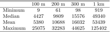
3.1 Variograms We calculated and plotted the em-pirical variograms from the residuals of the global model (Eq. 1) with different lags (Fig. 2). In the selection of the empirical variogram the balance between smooth-ness of the empirical variogram and the lag distance has to be found. With large lag distances the number of the point pairs in the bins increases (Table 4), the var-iogram smooth, but the smoothing can hide the actual small scale processes (trends) in the data. We selected the variogram with a lag distance of 200 m, which was just below the minimum inter-plot distance of 0.25 km in the study area (Table 1), because it was the shortest lag distance showing the trends and still the inter-stand and intra-stand variations do not overlap.
Table 4: Number of point pairs in the bins
100 m 200 m 300 m 1 km
Minimum 9 61 98 919
Median 4427 9809 15576 49340
Mean 5380 10688 16032 53439
Maximum 25075 32283 44625 125402
The first bin in the selected empirical variogram was at 10 m, where the semivariance was 0.006867 dm6/cm4.
The next semivariance at 277 m was 0.009045 dm6/cm4.
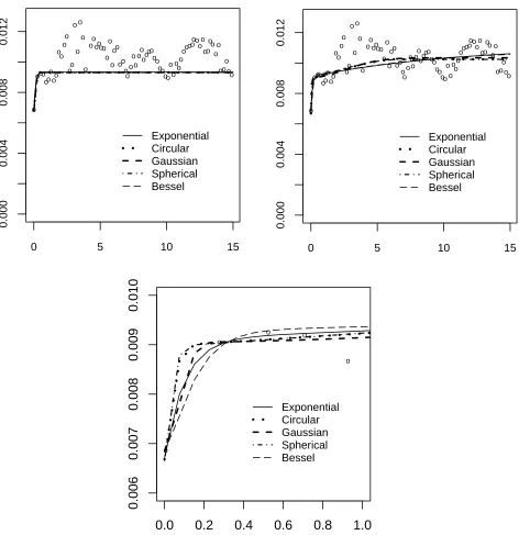
The change in level of the semivariance was so steep that we decided to fit a nested variogram model (Fig. 3b) in the empirical variogram, in which the short-range ‘intra-plot correlation’ with range of 100 m and the long-range ‘trend’ were separated, instead of simple variogram mod-els (Fig. 3a). The short-range component describes the nugget effect of the variogram model, and it was effective only for those trees in the same plot as the tree of predic-tion. The range of the short-range component was fixed at 100 m not fitted. The long-range model describes the correlation with the residuals in other plots and clusters. Its nugget effect was fixed to be zero. These two com-ponents formed the variogram model, which was then fitted to the empirical variogram.
o o o oo o o o ooooooooo
o ooo o o o o ooo o o o o o o o o o oo o o
ooooooooooooo oo o o oo o oo
oooooo oo o o oo oo o o o o o o o oo o ooooo ooooo o oo o o ooo o oo o o oooo o o o ooo o o ooo
o o o oo oo o o o o o o o o oo
ooooooo
0 5 10 15 Lag = 100 m
o oooooooo
ooo o oo o o o o o o
oooooo o
o
o oo
oo ooooooooo
oo oo
oooooooo oooo
ooooooooo oo
ooooo
0 5 10 15
0.000
0.005
0.010
0.015
0.020
Lag = 200 m
oooooo oo o o o oo o oooo ooooo
ooo ooooo
oooooooo oo ooooo
oooo
0 5 10 15 Lag = 300 m
o o
o o o o o
o o o o
o o o
o
0 5 10 15
0.000
0.005
0.010
0.015
0.020
Lag = 1 km
Figure 2: Empirical variograms with different lag distances from 100 m to 1 kilometre. Distance (km) is at x-axes and semivariance (dm6/cm4) at y-axes.
app. 5 km to 12 km (Fig. 3b; Table 5). We evaluated the models visually (Fig. 3b, c). All the models were almost similar at distances below 3 km. Though, there were differences, as you can see from the Fig. 3c for the first kilometre, it has to be remembered that the trees were located at plots (inter-plot distance 250-300 m, Table 1) and the small differences visible in the figure vanish.
The nugget effect was from 0.0065 to 0.0068 dm6/cm4 (Table 5). The circular, Gaussian and spherical vari-ogram models were almost identical for the remaining distances at ranges of 6.2, 3.7 and 6.8 km, and the sill approx. 0.01 dm6/cm4, showing the best fit in the
empirical semivariogram (Fig. 3a; Table 5). In con-trast, the exponential and Bessel models formed another group (Fig. 3a), which had a slightly higher sill of 0.011 dm6/cm4 and larger ranges than the previous group of
variogram models. We selected the spherical and Bessel models to describe the correlation in kriging calculation after this point. There was no evidence of anisotropy,
though directional variograms with several different di-vision of the space were compared.
3.2 Kriging In the 10-fold cross-validation, we split the data into 10 almost equally sized parts for which the predictions were made. Division into 10 folds was selected instead of the leave-one-out cross-validation be-cause it saved the calculation capacity considerably, but did not have remarkable impact on the results (Table 6). In the NFI9, the sampling design varied in differ-ent parts of the study area (NFI9, 2011; Table 1) which, in practice, meant that the number of neighbouring ob-servations as a function of distance from a tree varied. Therefore, we limited the neighbourhood by number of neighbours from 20 to 100 trees instead of by distance limitation.
The RMSE (root mean squared error) for the global model (Eq. 1) without RDIST was 0.1032 dm3/cm2and
o ooo
oo o
oo o
o o
o
oo o
o o
o
o oooooo
o o
o oo
oo o
o o
o o
oooooo oo
oo oo
o o
o o
o oooo
oo oo
oo oo
o o
oo o
oo
0 5 10 15
0.000
0.004
0.008
0.012
Exponential Circular Gaussian Spherical Bessel
o ooo
oo o
oo o
o o
o
oo o
o o
o
o oooooo
o o
o oo
oo o
o o
o o
oooooo oo
oo oo
o o
o o
o oooo
oo oo
oo oo
o o
oo o
oo
0 5 10 15
0.000
0.004
0.008
0.012
Exponential Circular Gaussian Spherical Bessel
o
o
o o
o
0.0
0.2
0.4
0.6
0.8
1.0
0.006
0.007
0.008
0.009
0.010
Exponential Circular Gaussian Spherical Bessel
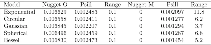
Table 5: Parameters of the fitted nested variogram models: nugget effect at the origins, partial sill (sill minus nugget effect) and ranges in kilometres for the short-range part (= 0.1 km) (Nugget O) and for the long-range part (Nugget M).
Model Nugget O Psill Range Nugget M Psill Range
Exponential 0.006629 0.002483 0.1 0 0.002097 11.8
Circular 0.006558 0.002411 0.1 0 0.001277 6.2
Gaussian 0.006845 0.002207 0.1 0 0.001294 3.7
Spherical 0.006496 0.002459 0.1 0 0.001287 6.8
Bessel 0.006830 0.002473 0.1 0 0.001454 5.2
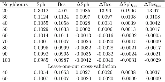
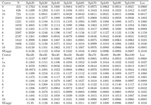
RMSPEs for kriging with different numbers of neigh-bours are shown in Table 6. The first estimates with 20 neighbours were unstable and the RMSPEs were high. With 30 neighbours the situation improved considerably, but with 40 neighbours the estimates and RMSPEs were stable in all folds and forestry centres (Table 7). Both variogram models gave similar results. In all, 60 neigh-bours were needed to obtain RMSPEs for kriging that were below the RMSE of a global regression model with both variogram models.
At the forestry centre level, the reference was a lo-calized regression model (R¨aty and Kangas, 2008). In this case it was simply Eq. 1, including the RDIST variable, re-fitted to the forestry centres. The refer-ence value here is 0.1016 dm3/cm2, the aggregate value
of the regional RMSEs of the locally re-fitted models. The kriging method had lower aggregate standard errors when the number of neighbours increased to 60 (Table 6). With regard to distances, this means an average kriging neighbourhood of 13.7 km (Table 3).
The regional biases, compared with the RMSPE in the same region (Eq. 16) with different variogram models, varied from -2.4% to 2.9% with neighbours from 40 to 100 (Table 8). The average bias was 0.8% for all forestry centres (calculated as the average of absolute value of biases proportional to the regional RMSPE). This shows the potential improvement in RMSPE if a regional factor were added to the model, i.e. this is the possibility for further localization after the kriging is carried out.
4
Discussion
One of the most important since this gives very dif-ferent results than universal kriging is fitting of the var-iogram model to the empirical varvar-iogram. It eventu-ally determines the weights given to neighbours. Pre-viously, Tomppo et al. (2001, Figs. 4, 5, p. 105) stud-ied the variograms and correlations of the mean volume and age in the NFI7 data in central Finland. They dis-covered a relatively large correlation (0.4–0.5) for both variables at 200 m. In the NFI9 the plot distance was increased to 300 m, and the correlations shown in the
above-mentioned figures were approximately 0.3–0.4 at that lag. The estimated correlations in this study at the origin were 0.37 for both variogram models (Table 5) (see Bailey and Gatrell, 1995), and at 300 m 0.12 and 0.16 for the spherical and Bessel models, respectively. However, as Tomppo et al. (2001) studied the correla-tion between the actual measurements, and we studied the correlation between the residuals, from which the obvious trends were already removed, this smaller value is understandable.
The changes in inter-cluster and inter-plot distances, i.e. in sampling design, have a direct impact on the var-iograms and kriging, however. First, when the distances to neighbours increase or, in other words, the proba-bility of having neighbours at short distances diminish, and therefore the SA between neighbouring observations and the pivot observation decrease. Second, since the SA weakens, the power of kriging also decreases; corrections based on the correlation between neighbours cannot be utilized as efficiently as previously. In our case, although the inter-plot distance was 250–300 m (Table 1), the SA could be found (Figs. 2b, c). Obviously, a zero correla-tion would mean there is no need for local adjustment in the first place, but the residuals are random.
Table 6: RMSPEs (dm3/cm2) for the kriging estimates with 10-fold cross-validation and leave-one-out cross-validation
of the form height with two variogram models, spherical (Sph) and Bessel (Bes), at global level, and differences to the global model RMSE (ΔSph and ΔBes) and to the forestry centre localized functions (ΔSphloc and ΔBesloc).
Neighbours Sph Bes ΔSph ΔBes ΔSphloc ΔBesloc
20 0.3012 14.07 0.1985 13.96 0.1996 13.97
30 0.1124 0.1124 0.0097 0.0097 0.0108 0.0108
40 0.1055 0.1058 0.0028 0.0031 0.0039 0.0042
50 0.1029 0.1033 0.0002 0.0006 0.0013 0.0017
60 0.1014 0.1011 -0.0013 -0.0016 -0.0002 -0.0005
70 0.1001 0.1007 -0.0026 -0.0020 -0.0015 -0.0009
80 0.0995 0.0999 -0.0032 -0.0028 -0.0021 -0.0017
90 0.0992 0.0995 -0.0035 -0.0032 -0.0024 -0.0021
100 0.0985 0.0987 -0.0042 -0.0040 -0.0031 -0.0029
Leave-one-out cross-validation
40 0.1054 0.1053 0.0027 0.0026 0.0038 0.0037
60 0.1007 0.1007 -0.0020 -0.0020 -0.0009 -0.0009
is approached is gentle, a relatively high weight is given to observations far from the origin. The Bessel model is an example of this; it approaches its sill asymptotically and therefore the range given is only about one-fourth of an effective range (Webster and Oliver, 2007), whereas the range given for the spherical model equals the effec-tive range. Considering this property, the ranges for the variogram models were 6.8 km and 5.2 km for the spher-ical and Bessel variogram models, respectively. In prac-tice, this means that all observations belonging to the same cluster were correlated and the correlations were extended to neighbouring clusters with both variogram models, as well. With the Bessel variogram model, small weights were given for plots in the clusters behind the neighbouring clusters and even further away, because the effective range was over 20 km. In fact, observations be-yond the effective range may also bear weight, since the proportion of the nugget effect of the sill is larger than that of the partial sill (e.g. Webster and Oliver 2007, p. 168).
The fluctuation and periodicity in the empirical vari-ogram after 5 km cannot be explained with small num-bers of pairs in the bins (Fig. 3b; Table 4), nor with the anisotropy of the variogram, but it could have resulted from the natural extent of forest patterns and compart-ments. In empirical variograms the estimates are nor-mally strongly autocorrelated (Jowett, 1955; Chil`es and Delfiner, 1999, p. 111, 205; Schabenberger and Pierce, 2002, p. 617; Diggle et al., 2003, Fig. 2.10) and this cor-relation, combined with the clustered empirical design, could be an explanation to the apparent periodicity in empirical variograms. Schabenberger and Pierce (2002) call this relay effect. Nevertheless, the variogram mod-elling at short distances is more important in respect to
kriging than the periodicity.
Kriging in the local neighbourhood could have been implemented either by setting the maximum distance limit to the neighbourhood, possibly combined with the requirement for a minimum number of neighbours, or by setting directly the number of neighbours. We selected the latter course; the kriging neighbourhoods were lim-ited directly by the number of neighbours. Kallas et al. (2003) used four neighbours in their study, while Web-ster and Oliver (2007) suggested that usually 20 neigh-bours are sufficient. Given this clustered data with single data points situated on islands or near the great inland lakes, 30 neighbours were needed to obtain the first sta-ble estimates for the estimated pivot. On average this meant a 10-km circular neighbourhood. To obtain lower RMSPEs than the global or the regionally localized mod-els (Tables 6; 7) the distances increased up to 13.7 km (Table 3).
The neighbourhood distances and RMSPEs varied in different forestry centres, but a small neighbourhood in kilometres did not automatically mean low RMSPEs. Good examples of these contrasting results were forestry centres 1b and 6; the first had only a few observations predicted from the largest neighbourhoods in the dataset (max. 48 km), but its RMSPEs were among the lowest (Tables 3; 7). The second sub-area, forestry centre 6, had the smallest neighbourhoods (max. 22 km), but the RMSPE was one of the largest. Some explanation to these differences could have resulted from the differences in form height in both sub-areas. The range of form heights is smallest in the forestry centre 1b whereas in forestry centre 6 it is the second largest.
Table 7: Localization results (dm3/cm2) at forestry centre level by 10-fold cross-validation with different variogram
models (Sph = spherical and Bes = Bessel followed by the number of neighbours in kriging), and regression model localization (Loc) from R¨aty and Kangas (2008).
Centre N Sph20 Sph30 Sph40 Sph50 Sph60 Sph70 Sph80 Sph90 Sph100 Loc
0 455 0.1763 0.1046 0.1008 0.0984 0.0974 0.0975 0.0963 0.0954 0.0921 0.0968
1a 826 0.1499 0.1293 0.1101 0.1056 0.1051 0.1043 0.1043 0.1023 0.1012 0.1037
1b 723 0.1131 0.0941 0.0871 0.0828 0.0843 0.0811 0.0821 0.0815 0.0806 0.0817
2 2383 0.1618 0.1077 0.1009 0.0986 0.0975 0.0969 0.0953 0.0959 0.0946 0.1002
3 1221 0.1455 0.1188 0.1115 0.1105 0.1094 0.1095 0.1086 0.1080 0.1071 0.1060
4 1659 0.4865 0.1190 0.1114 0.1098 0.1066 0.1063 0.1057 0.1059 0.1053 0.1065
5 1622 0.1485 0.1172 0.1061 0.1047 0.1025 0.1017 0.0995 0.1000 0.0994 0.0989
6 2397 0.2028 0.1246 0.1196 0.1167 0.1156 0.1137 0.1127 0.1132 0.1126 0.1159
7 2197 0.1381 0.0969 0.0916 0.0879 0.0860 0.0846 0.0842 0.0830 0.0831 0.0832
8 1842 0.2999 0.1069 0.1007 0.1001 0.0985 0.0975 0.0969 0.0963 0.0962 0.1035
9 1606 0.1333 0.1130 0.1071 0.1041 0.1018 0.0999 0.1010 0.1006 0.1003 0.1040
10 2244 0.6138 0.1101 0.1062 0.1017 0.1007 0.0976 0.0980 0.0966 0.0958 0.0985
SEaggr 0.3136 0.1122 0.1058 0.1032 0.1016 0.1002 0.0996 0.0993 0.0987 0.1016
Centre Bes20 Bes30 Bes40 Bes50 Bes60 Bes70 Bes80 Bes90 Bes100 Loc
0 0.1247 0.1067 0.1020 0.0982 0.0976 0.0965 0.0954 0.0953 0.0945 0.0968
1a 0.1383 0.1151 0.1106 0.1058 0.1052 0.1049 0.1044 0.1032 0.1032 0.1037
1b 0.1059 0.0921 0.0856 0.0841 0.0828 0.0844 0.0816 0.0821 0.0812 0.0817
2 39.8974 0.1095 0.1022 0.0988 0.0964 0.0970 0.0959 0.0954 0.0944 0.1002
3 0.1499 0.1216 0.1131 0.1127 0.1112 0.1103 0.1086 0.1089 0.1077 0.1060
4 0.1472 0.1186 0.1117 0.1097 0.1065 0.1066 0.1063 0.1063 0.1050 0.1065
5 0.1486 0.1148 0.1078 0.1067 0.1027 0.1018 0.1001 0.0998 0.0997 0.0989
6 0.1584 0.1268 0.1210 0.1150 0.1135 0.1132 0.1131 0.1140 0.1117 0.1159
7 0.1206 0.0972 0.0904 0.0872 0.0847 0.0848 0.0835 0.0834 0.0837 0.0832
8 0.1336 0.1078 0.1015 0.0999 0.0983 0.0990 0.0980 0.0965 0.0958 0.1035
9 0.1485 0.1153 0.1058 0.1039 0.1028 0.1015 0.1018 0.1013 0.1007 0.1040
10 0.1436 0.1086 0.1045 0.1041 0.1009 0.0990 0.0987 0.0966 0.0960 0.0985
SEaggr 15.95 0.1126 0.1061 0.1034 0.1011 0.1007 0.1000 0.0996 0.0987 0.1016
kriging. In this case, we had 10-fold cross-validation in which 10% of the population was omitted at time. In other words, 90% of the data was used to predict each observation. Since the data were divided randomly, the resulting divisions should also have been irregular and the neighbourhoods of the single points should not have changed, i.e. the points should have had on average 90% of the original neighbours as the same distances had before division. To judge the equality in divisions, we accounted and compared the RMSPEs for every fold included in the calculations. When the number of neigh-bours increased, the variability in RMSPEs in the dif-ferent folds decreased. Since the folds were similar, we assumed that the division into 10 folds was neutral with respect to the prediction.
We used regionally localized regression models as ref-erences for the kriging estimates (R¨aty and Kangas, 2008). The regions were the forestry centres (Fig. 1b) and the model (Eq. 1) was the same for every centre;
it was only fitted for every area separately. After re-fitting, there was no regional bias in the local estimates. Kriging, on the other hand, was not bounded to the sub-areas, but the results were also reported by the forestry centres. The bias in kriging estimates was below 1% of the RMSPE of the forestry centres (Table 8). There-fore, adding a local regional variable to KED would only slightly improve the estimates.
Table 8: Regional relative biases in estimates as percentages of RMSPE of the kriging estimate, Biasrel, at the forestry centre.
Centre Sph20 Sph30 Sph40 Sph50 Sph60 Sph70 Sph80 Sph90 Sph100
0 4.7 -1.8 -0.7 0.7 -1.5 1.1 -0.8 -2.4 -1.3
1a 2.8 3.6 1.3 0.0 -0.7 -0.3 -0.5 -0.1 -1.2
1b 4.2 1.3 0.3 -0.4 0.3 -0.4 -1.2 0.3 0.1
2 2.0 0.9 1.2 1.2 0.7 1.1 0.7 1.1 1.7
3 -9.0 0.6 0.5 -0.6 -0.7 -0.1 0.0 0.7 0.1
4 0.8 2.3 1.8 1.1 2.2 1.3 1.2 1.3 1.6
5 -1.8 2.0 1.1 0.2 0.3 0.4 0.7 -0.4 -0.2
6 0.0 0.8 -0.3 -0.4 -1.2 -0.9 -0.7 -0.5 -0.6
7 -2.9 -0.6 1.4 0.2 0.4 0.6 0.3 0.1 -0.1
8 0.8 0.1 -0.7 0.3 -0.5 -1.7 -0.6 -0.7 -0.7
9 12.5 2.2 2.9 1.2 0.8 1.0 0.9 0.8 0.5
10 -0.2 2.0 1.2 0.9 -0.1 0.8 1.4 1.2 1.1
Centre Bes20 Bes30 Bes40 Bes50 Bes60 Bes70 Bes80 Bes90 Bes100
0 4.7 0.2 -1.7 0.4 -0.2 -0.1 0.1 -1.0 -0.9
1a 2.6 3.3 1.4 -0.7 0.8 -0.6 -1.7 -0.7 -1.7
1b 1.1 0.5 0.4 0.8 1.9 2.0 1.2 0.6 1.2
2 -2.1 0.5 0.4 -0.3 -0.5 -0.2 0.5 -0.5 -0.4
3 -0.1 -0.9 1.0 2.5 1.8 0.9 0.3 0.4 0.3
4 2.1 0.1 0.3 0.0 0.3 0.7 1.1 0.2 0.1
5 2.6 1.6 2.1 1.1 2.0 1.5 0.4 1.9 1.1
6 -1.8 0.7 0.7 0.8 0.3 0.3 0.3 0.1 0.1
7 2.6 2.7 0.5 -0.9 -0.9 -1.1 -1.0 -1.0 -0.9
8 1.0 -0.4 0.2 0.4 0.7 0.2 -0.2 0.7 0.3
9 3.3 0.7 0.5 -0.2 -1.1 -0.5 -0.2 -0.5 -1.6
10 0.1 1.8 2.2 1.5 0.2 1.4 0.4 0.9 0.6
forests in forestry centre 3 differed from that in other forestry centres, comprising only 38% of the forested land area (Fig. 1 in Korhonen et al., 2007), whereas in other forestry centres the proportion was considerably higher, varying from 47% to 78%. Also the distances to the neighbours are among the largest (the minimum, me-dian and mean distances are large even though the max-imums are quite small, Table 3) and therefore the correc-tion the neighbourhood provides is one of the smallest.
We based this study on previous results (R¨aty and Kangas, 2007; 2008; 2010) and used here the same re-gression model in KED to predict the form height of a tree. KED is only one kriging method among others, and comparing different methods and trend model de-velopment for the kriging purpose, as Musio et al. (2004) did, could have given more information to carry out the prediction. To save computing capacity, we made two restrictions: the kriging was limited to a local neighbour-hood and the folds in cross-validation were increased to 10% of the total number of observations instead of one observation. Limitation of the neighbourhood was rea-sonable, since the idea was to use the closest neighbours
in prediction. However, the Bessel variogram model weighted all observations in the study area, although the weighting was only fractional beyond an effective range and the prediction stabilized as the number of neigh-bours increased. Kriging proved to be a better solution than the regression model. However, it is possible that using a more flexible model as a global model might further improve the results. Thus, the next step could be a comparison between kriging and nonparametric k-nearest neighbours (k-NN) methods (e.g. Moeur and Stage, 1995).
5
Conclusions
neigh-bours and sparse sampling design. The method could be improved, e.g. by adding to the kriging informa-tion on the other tree species in the neighbourhood. It would also be interesting, though complicated, to study a relationship between local ecological differences and the modelling in the forestry centres. Since there were forestry centres where the regional re-fitting of the global model was better than the KED, combination of these two methods is also feasible.
References
Anselin, A. 1995. Local indicators of spatial association—LISA. Geogr. Anal. 27: 93–115.
Bailey, T.C. and A.C. Gatrell. 1995. Interactive spatial data analysis. Harlow: Longman. 413 p.
Boots, B. 2002. Local measures of spatial association. Ecoscience 9: 168–176.
Chile‘s, J.-P. and P. Delfiner. 1999. Geostatistics: mod-eling spatial uncertainty. Wiley, New York. ISBN: 0-471-08315-1. 695 p.
Cliff, A.D. and J.K. Ord. 1981. Spatial processes: models and applications. Pion Limited, London. 266 p.
Cressie, N.A.C. 1991. Statistics for spatial data. Wiley, New York (NY). 900 p.
Diggle, P.J., P.J. Ribeiro Jr. and O.F. Christensen. 2003. An introduction to model-based geostatistics P. 44-86 in Spatial Statistics and Computational Methods, Møller, J. (ed.) Lecture Notes in Statistics Vol. 173. Springer, New York. ISBN:9780387001364.
Fuentes, M., T.G.F. Kittel and D. Nychka. 2006. Sen-sitivity of ecological models to their climate drivers: statistical ensembles for forcing. Ecol. Appl. 16(1): 99-116.
Getis, A. and J.K. Ord. 1992. The analysis of spatial association by use of distance statistics. Geogr. Anal. 24: 189-206.
Getis, A. and J.K. Ord. 1996. Local spatial statistics: an overview. P. 261–278 in Spatial analysis: modelling in a GIS environment, Longley, P.A. and M. Batty. (eds.). GeoInformation International, Cambridge.
Hamann, A., M.P. Koshy, G. Namkoong and C.C. Ying. 2000. Genotype x environment interactions in Alnus
rubra: developing seed zones and seed-transfer guide-lines with spatial statistics and GIS. For. Ecol. Man-age. 136: 107-119.
Hengl, T., G.B.M. Geuvelink and A. Stein. 2003. Comparison of kriging with external drift and regressikriging. Technical note, ITC. Available on-line at http://www.itc.nl/library/Academic output/; last accessed Feb. 26, 2011.
Isaaks, E.H. and R.M. Srivastava. 1989. An introduc-tion to applied geostatistics. Oxford University Press, Oxford (NY). 561 p.
Johannesson, G., N. Cressie and H.-C. Huang. 2007. Dy-namic multi-resolution spatial models. Environ. Ecol. Stat. 14: 2-25.
Johnson, E.W. 2000. Forest sampling desk reference. CRC Press, Boca Raton. 985 p.
Jowett, G.H. 1955. Sampling properties of local statistics in stationary stochastic series. Biometrika 42: 160-169.
Kallas, M.A., R.M. Reich, W.R. Jacobi and J.E. Lundquist. 2003. Modeling the probability of observ-ing Armillaria root disease in the Black Hills. Forest Pathol. 33: 241-252.
Kangas, A. and K.T. Korhonen. 1995. Generalizing sam-ple tree information with semiparametric and para-metric models. Silva Fennica 29:151–158.
Korhonen, K.T. 1993. Mixed estimation in calibration of volume functions of Scots pine. Silva Fennica 27:269– 276.
Korhonen, K.T., A. Ihalainen, J. Heikkinen, H. Hent-tonen and J. Pitk¨anen. 2007. Suomen mets¨avarat mets¨akeskuksittain 2004–2006 ja mets¨avarojen kehi-tys 1996–2006. Mets¨atieteen aikakauskirja 2B/2007: 149-213 (in Finnish).
Magnussen, S., E. Næsset and M.A. Wulder. 2007. Effi-cient multiresolution spatial predictions for large data arrays. Rem. Sens. Environ. 109: 451–463.
Moeur, M. and A.R. Stage. 1995. Most similar neighbor: an improved sampling inference procedure for natural resource planning. For. Sci. 41(2): 337-359.
Musio, M., N. Augustin, H.-P. Kahle, A. Krall, E. Kublin, R. Unseld and K. von Wilpert. 2004. Pre-dicting magnesium concentration in needles of Silver fir and Norway spruce – a case study. Ecol. Modell. 179: 307-316.
Nanos, N. and G. Montero. 2002. Spatial prediction of diameter distribution models. For. Ecol. Manage. 161: 147-158.
NFI9. 2011. 9th National Forest Inventory. Finnish Forest Research Institute. Available online at http://www.metla.fi/ohjelma/vmi/vmi9-info-en.htm; last accessed Feb. 26, 2011.
Pebesma, E.J. and C.G. Wesseling. 1998. Gstat, a pro-gram for geostatistical modelling, prediction and sim-ulation. Comput. Geosci. 24(1): 17–31.
Pebesma, E.J. 2004. Multivariable geostatistics in S: the gstat package. Comput. Geosci. 30(7): 683-691.
R Development Core Team. 2009. R: A language and environment for statistical computing. R Foundation for Statistical Computing, Vienna, Austria. ISBN 3-900051-07-0. Available online at http://www.R-project.org; last accessed Feb. 26, 2011.
R¨aty, M. and A. Kangas. 2007. Localizing general mod-els based on local indices of spatial association. Euro-pean Journal of Forest Research 2/2007:279 – 289.
R¨aty, M. and A. Kangas. 2008. Localizing global models with classification and regression trees (CART). Scand J Forest Res 5/23: 419-430.
R¨aty, M. and A. Kangas. 2010. Segmentation of Model Localization Sub-areas by Getis Statistics. Silva Fenn 44(2): 303-317.
Sales, M.H., C.M. Souza Jr., P.C. Kyriakidis, D.A. Roberts and E. Vidal. 2007. Improving spatial distri-bution estimation of forest biomass with geostatistics: A case study for Rondˆonia, Brazil. Ecol. Modell. 205: 221-230.
Schabenberger, O. and C. A. Gotway. 2005. Statis-tical methods for spatial data analysis. Chapman &Hall/CRC, Boca Raton, FL. 488 p.
Schabenberger, O. and F. J. Pierce. 2002. Contemporary statistical models for the plant and soil sciences. CRC Press, Boca Raton, FL. 738 p.
Shiver, B.D. and B.E. Borders. 1996. Sampling tech-niques for forest resource inventory. Wiley, New York. 356 p.
Staelens, J., L. Nachtergale and S. Luyssaert. 2004. Pre-dicting the spatial distribution of leaf litterfall in a mixed deciduous forest. For. Sci. 50(6): 836-847.
Tomppo, E., H. Henttonen and T. Tuomainen. 2001. Valtakunnan metsien 8. inventoinnin menetelm¨a ja tu-lokset mets¨akeskuksittain Pohjois-Suomessa 1992-94 sek¨a tulokset Etel¨a-Suomessa 1986-92 ja koko maassa 1986-94. Mets¨atieteen aikakauskirja 1B/2001: 99-248 (in Finnish).