Solution of different multi-criteria decision making engineering problems by PROMETHEE II and VIKOR

Solution of different multi-criteria decision

making engineering problems by

PROMETHEE II and VIKOR

A Report submitted to the

National Institute of Technology, Rourkela In partial fulfilment of the requirements

of

Bachelor of Technology (Mechanical Engineering)

By

ADITYA KUMAR GAUTAM

Roll no. 110ME0293

UNDER THE GUIDANCE

OF:-Prof. Saroj Kumar Patel

DEPARTMENT OF MECHANICAL ENGINEERING

NATIONAL INSTITUTE OF TECHNOLOGY, ROURKELA -769008

B. Tech. Project Report

2014

Mechanical Engineering Department, NIT Rourkela Page 2

Certificate of Approval

This is to certify that the thesis entitled

Solution of different

multi-criteria decision making engineering problems by PROMETHEE II

and VIKOR

submitted by

Aditya Kumar Gautam

has been carried out

under my supervision in partial fulfilment of the requirements for the

Degree of Bachelor of Technology (B. Tech.) in Mechanical

Engineering at National Institute of Technology, Rourkela, and this

work has not been submitted elsewhere before for any other academic

degree/diploma.

---

Dr. Saroj Kumar Patel,

Associate Professor,

Department of Mechanical Engineering,

National Institute of Technology, Rourkela.

Date: -

B. Tech. Project Report

2014

Mechanical Engineering Department, NIT Rourkela Page 3

Acknowledgement

I am very thankful to my project guide Dr. Saroj Kumar Patel,

Associate Professor, Department of Mechanical Engineering,

National institute of technology, Rourkela, to introduce me to this

topic and help me in any way he could by encouraging me

cooperating with me in my work and giving intellectual suggestions

for the completion of my project work.

I would also like to thank Dr. K. P. Maity, Professor and Head of

Department,

Mechanical

Engineering,

National

Institute

of

Technology, Rourkela, for providing necessary information and

guidance for the completion of my project work.

I also want to express my sincere gratitude to all my friends for

supporting me and assisting me throughout my project work.

Aditya Kumar Gautam,

Department of Mechanical Engineering,

B. Tech. Project Report

2014

Mechanical Engineering Department, NIT Rourkela Page 4

Abstract

In our day to day life we come across situations in which we have a

number of choices available in front of us and it is difficult to choose

among them on the basis of a single criterion. Different alternatives

have different attributes related to them so it is important for the

decision maker to weigh all the alternatives and come up with a

common index on the basis of which he can compare his alternatives.

In this thesis, to encounter with such problems, multi criteria decision

making methods have been used to come up with the best alternative.

Two methods namely PROMETHEE II (preference ranking

organization method for enrichment evaluation) and VIKOR

(višekriterijumsko kompromisno rangiranje) have been used to solve

different engineering problems ranging from selection of machining

parameters to choosing a supplier for an industry. PROMETHEE II

uses the outranking method for the ranking of alternatives and

VIKOR is a compromise solution method. Four selected real life

problems have been solved by both the methods and the results have

been compared with each other.

B. Tech. Project Report

2014

Mechanical Engineering Department, NIT Rourkela Page 5

Contents

TOPIC

PAGE NO.

Title Page

1

Certificate of Approval

2

Acknowledgement

3

Abstract

4

Contents

5

1. Introduction

6

2. Literature Review

8

3. Calculation of Weights

10

4. PROMETHEE II

11

5. VIKOR

13

6. Problems and their Solutions

14

6.1 Use of PROMETHEE II and VIKOR in the selection

14

of machining parameters for Inconel 718.

6.2 Implementation of MCDM methods for

19

selection of a warehouse Location.

6.3 Cutting tool material selection using

21

PROMETHEE II and VIKOR methods.

6.4 Use of a MCDM approach for selection of

27

suppliers in auto industry.

7. Conclusion

29

B. Tech. Project Report

2014

Mechanical Engineering Department, NIT Rourkela Page 6

1. Introduction

Making a choice about a certain thing is very difficult in this world because we have a variety of choices and we make our choices based on various criteria having some positive and some negative attributes. We make our choices by comparing and ranking objects according to criteria defined by us, such as while choosing a car we look through various properties of the car like it’s top speed, its comfort level, safety, cost, mileage etc. and after that we make our choice depending on what is most important for us. One of the various methods to rank, compare and order several alternatives is based on the notion of “Multiple Criteria Decision Making (MCDM)”. It has been recognized as an efficient statistical method in which we can combine different indices of various criteria for all the choices available to us into a single feasible data which can help in comparing and ranking the objects. A typical MCDM problem has a series of alternatives with different criteria which have to be assessed using different methods and then the alternatives have to be ranked.

The MCDM problems can be mainly classified into two types [1]: -

 Multi-Criteria evaluation problems: - Here the number of alternatives is finite and are clearly known at the beginning of the solution process.

 Multi-Criteria design problems: - The alternatives here are not explicitly known. We have an infinite number of alternatives available or are very typically large in number if countable.

MCDM problems can be solved by methods that are commonly classified based on the timing of preference information obtained from the decision maker. Criterion space or the decision space can be used to represent a MCDM problem. But if the criteria are combined together using a linear weighted function than it is possible to represent the problem in weighted space. Various analytical methods have been proposed to give a suggestion in conflict management situations by a large number of papers. Among these approaches available to make a difficult choice involving various alternatives and criteria, one of the most appropriate is multi-criteria decision making. The various steps involved in a MCDM problem are [2]: -

a) The system relations attributes are obtained that relate the system capability to reach the goals.

b) Various alternatives are then generated to reach the goal.

c) The performance function of these alternatives for every criterion available is obtained.

d) Applying the chosen method of MCDM to solve for the best alternative among the available ones.

e) Accepting the best alternative available to reach the goal.

f) If our aim is not fulfilled we gather more data about the model and go for next iteration of the MCDM process.

B. Tech. Project Report

2014

Mechanical Engineering Department, NIT Rourkela Page 7

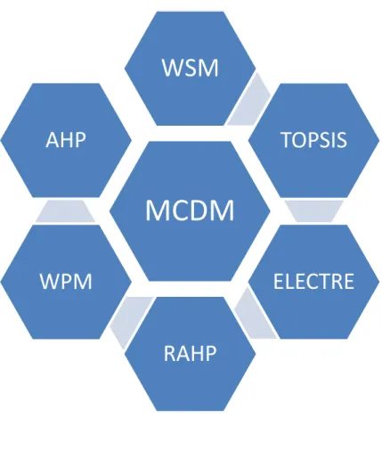
The steps a) and e) are taken care of by upper level decision makers and the rest of the steps are carried upon by the engineers. Here in this thesis out of various MCDM methods available PROMETHEE II and VIKOR method have been used to encounter various engineering problems. Various other MCDM methods are shown below in Figure 1. Various engineering problems relating to determination of machining parameters, determinations of a warehouse location and problem regarding choosing a vendor has been taken up and have been solved by using the above mentioned two methods. To determine the weightage of various criteria AHP has been used. The main aim of the project is to determine the ranks of different alternatives available to us in the chosen problems and analyse and compare the results obtained by both the processes.

Figure 1.Classification of MCDM methods

MCDM

WSM

TOPSIS

ELECTRE

RAHP

WPM

AHP

B. Tech. Project Report

2014

Mechanical Engineering Department, NIT Rourkela Page 8

2. Literature Review

The main aim of this literature review is to determine the importance of various MCDM methods in helping us to make a choice based on various criteria from different available alternatives. Many engineering problems have been taken up by various authors and in all those problems MCDM methods have been used to determine the best alternative may it be machining parameters or selection of cutting tool etc.

Chauhan and Vaish [3] used various MCDM approach for the selection of hard coating material. Various materials have given rise to intense research in the field of material selection. Technique for order preference by similarity to ideal solution (TOPSIS) was used for ranking these materials by him. He used material selection charts (Ashby approach) to select hard coating materials. Pareto-optimal hard coating materials were determined for trade-off between hardness (H), H/E and H3/E2 (E: Young’s modulus). Çalıskan [4] used EXPROM2 (preference ranking organization method for enrichment evaluation), TOPSIS (technique for order performance by similarity to ideal solution) and VIKOR for the selection of boron based tribological hard coatings. The alternatives consisted of multicomponent nanostructured TiBN, TiCrBN, TiSiBN and TiAlSiBN coatings and the material selection criteria were hardness (H), young’s modulus (E), elastic recovery, friction coefficient, critical load, H/E and H3/E2 ratios.

Ren et al. [5] studied four biomass-based technologies including pyrolysis, conventional gasification, supercritical water gasification and fermentative hydrogen production and used a novel fuzzy multi-actor multi-criteria decision making method to determine that the best process was biomass gasification for sustainable production of hydrogen. Keramati et al. [6] proposed a method based on the grouped fuzzy decision-making approach in order to evaluate and rank the most suitable suppliers for outsourcing activities in Iran national steel industrial group. The proposed method was used and experts presented their views in linguistic words, a range of numbers, deterministic or fuzzy numbers. Thereafter every supplier was ranked based on the available model criteria. The most effective criterion for determining the supplier selection was also determined by him. Adhikary and Kundu [7] used MCDM methods in selection of the various small parameters involved in a small hydropower project where the investment is a bit risky and depends on different factors and policies.

B. Tech. Project Report

2014

Mechanical Engineering Department, NIT Rourkela Page 9

Various engineering problems as mentioned above have been solved by using different MCDM techniques. Here this project thesis also involves solution of different engineering problems which have been solved by the help of different MCDM techniques by using PROMETHEE II and VIKOR methods. The different engineering problems taken up are mentioned below: -

a) Thirumalai and Senthilkumaar [8] conducted experiment for the selection of machining parameters for Inconel 718 and optimized the experimental values to obtain non dominated solutions and then ranked the different alternatives available on the basis of various criteria using TOPSIS.

b) Ozcan et al. [9] used AHP, TOPSIS, ELECTRE and Grey Theory to make a comparative analysis of the 4 choices available for the warehouse selection based on the criteria of unit price, stock holding capacity of warehouse, average distance to shops , average distance to main suppliers and the movement flexibility of the warehouse.

c) Maity et al. [10] determined the process of selecting the cutting tool material by using the grey complex proportional assessment (COPRAS-G) method and assessed all the alternatives available for the selection based on the decided criteria.

d) Shahroudi and Rouydel [11] proposed an integrated approach of ANP- TOPSIS to evaluate suppliers in Iran’s auto industry. Selection of a supplier in any industry is a very difficult task and we have to consider various factors such as cost, on time delivery etc. to determine the supplier and the amount of supply we should order from various suppliers. This paper shows a detailed study for selection of a supplier for auto industry.

B. Tech. Project Report

2014

Mechanical Engineering Department, NIT Rourkela Page 10

3. Calculation of Weights

As mentioned earlier to determine the rank of different alternatives available we need to determine the weights of each criterion. Weightage can be defined as the importance of those criteria for determining our choice. Both AHP and ENTROPY methods can be used to determine the weightage of different criterion. These two methods can be used together or separately as required. In this thesis AHP method has been used to determine the weightage of each criterion in different problems.

AHP METHOD

Saaty [12] developed the AHP method to model subjective decision-making processes based on MCDM in a hierarchical system [13]. This strategy involves fundamentally three standards: firstly, structure of the model; also, relative judgment of the options and the criteria; in conclusion, amalgamation of the necessities. For correlation of a set of n criteria pairwise as indicated by their relative significance weights, the pairwise examination matrix is utilized and it can be represented as [13]: -

where the criterions are denoted by a1, a2, . . . ,an. The relative importance between two

criterions is rated by use of a scale with the digits 1, 3, 5, 7 and 9, where 1 denotes ‘‘equally important’’, 3 for ‘‘slightly more important’’, 5 for ‘‘strongly more important’’, 7 for ‘‘demonstrably more important’’ and 9 for ‘‘absolutely more important’’. The digits 2, 4, 6 and 8 are used to facilitate a compromise between slightly differing judgments [14]. These comparative weights are obtained by finding the eigenvector w with respective λmax that

satisfies A*w = λmax* w, where λmax is the largest eigenvalue of the matrix A. In order to

ensure the consistency of the subjective perception and the accuracy of the comparative weights, the consistency index (C.I.) and the consistency ratio (C.R.) are calculated. The consistency index (C.I.) is CI = (λmax-n)/(n-1) where n is the number of the criterions. The

numerical value of the C.I. should be lower than 0.1 for confident result. The consistency ratio (C.R.) can be calculated as:

CR = CI/RI.

The R.I. is determined for different size matrixes, and its value is 1.25 for a 6 *6 matrix. The C.R. should be under 0.1 for a reliable result [13].

B. Tech. Project Report

2014

Mechanical Engineering Department, NIT Rourkela Page 11

4. PROMETHEE II

The EXPROM2 method is the modified and extended version of PROMETHEE II method which is based on the notion of ideal and anti-ideal solutions. In this method, first a basic concept of fuzzy outranking relation is considered and built into each criterion by pairwise comparison measures for alternatives to different relation- degrees in each other. These different relation-degrees are then used to set up different orders on a finite set of feasible solutions. These different relation-degrees are then used to set up different orders on a finite set of feasible solutions [13].

The steps of PROMETHEE II method are summarized below [15-17]: -

 First, the normalization of the decision matrix for beneficial criteria and non-beneficial criteria is performed by the below mentioned equations: -

where xij designates the performance measure of ith alternative with respect to jth criterion

and rij shows the normalized value of xij.

 The differences in criteria values (dj) between different alternatives pair-wise are

calculated.

 In order to calculate preference function Pj (i, i’) the below mentioned equations are used. The preference functions are utilized for the measurement of the degree by which alternative i dominates alternative i’ for jth criterion. Usual criterion, which is one of the generalized preference functions, is used here.

 The weak preference index (aggregated preference function), WPij(i, i’), is calculated

using following equation: -

where wj is the weight of jth criterion obtained by the compromised weighting method.

B. Tech. Project Report

2014

Mechanical Engineering Department, NIT Rourkela Page 12

where Lj indicates the limit of preference (0 for usual criterion preference function, and

indifference values for other five preference functions) and dmj is the difference between

ideal and anti-ideal values of jth criterion. Strict preference index, SP(i, i’), is,

 Total preference index, TPj(i, I’), is,

 Leaving (positive) flow for ith alternative is obtained by the below mentioned and shows how much an alternative dominates the other alternatives.

 Entering (negative) flow for ith alternative is obtained by the below mentioned and expresses how much an alternative is dominated by the other alternatives.

 In order to obtain the complete pre-order, the net outranking flow, φ(i), for each alternative is calculated.

B. Tech. Project Report

2014

Mechanical Engineering Department, NIT Rourkela Page 13

5. VIKOR

The VIKOR, the compromise solution method, was introduced as an applicable technique to implement within MCDM [18].

The main procedure of the VIKOR method is described below:

 First, the best, i.e. (xij)max and the worst, i.e. (xij)min values of all criteria are

determined from decision matrix.

 The values of Ei and Fi are calculated from equations below respectively.

 The values of Pi are calculated.

where Ei-max designates the maximum value of Ei, and E designates the minimum value of E i-min; Fi-max is the maximum value of Fi, and Fi-min is the minimum value of Fi, v is used as the

weight of the strategy of ‘the majority of criteria’. The value of v is usually taken as 0.5, while it can take any value from 0 to 1.

 According to the values of Pi, Ei and Fi, the alternatives are separately arranged in the

ascending order in order to obtain three ranking lists. The compromise ranking list for a given v is obtained by ranking according to Pi measures. The best alternative is

B. Tech. Project Report

2014

Mechanical Engineering Department, NIT Rourkela Page 14

6. Problems and their Solutions

6.1 Use of PROMETHEE II and VIKOR in the selection of machining

parameters for Inconel 718.

The set of non-dominated solutions obtained using the non-sorted genetic algorithm for multi-objective functions is taken from the paper available [8] and multi-criteria decision making (MCDM) is used to determine a single solution from the set of non-dominated solutions. The experiment involves the high-speed using carbide cutting tool for the machining of Inconel 718 where 6 output parameters are measured that are considered as attributes against the process variables of cutting speed (v), feed (f), and depth of cut (a). The attributes or the output parameters are surface roughness (Ra), flank wear (Vb), tool life (TL), cutting force (F), power consumption (P) and material removal rate (MRR). The objective functions Ra, Vb, F, and P are non-beneficial (minimum values are better) whereas attributes TL and MRR are beneficial (maximum values are better). First of all the weights are calculated using the AHP method and then PROMETHEE II and VIKOR methods described above are used to get the ranks of different alternatives.

Calculation of Weight

Table 1.Relative attribute matrix [8]

Attribute Ra F P TL MRR Vb Ra 1 3 3 1 2 1 F 1/3 1 1 1/3 2/3 1 P 1/3 1 1 1/3 2/3 1 TL 1 3 3 1 2 1 MRR 1/2 2/3 2/3 ½ 1 1 Vb 1 1 1 1 1 1

Table 1 tabulates the pairwise attribute matrix. The above matrix of attributes is then normalized by following the steps above mentioned in the AHP methods to obtain the weights of different criteria. The normalized matrix is first found by calculating the sum of each column and dividing the attribute value with the resultant and then for finding the weights we find the average of each row which gives us the respective weights of criteria.

B. Tech. Project Report

2014

Mechanical Engineering Department, NIT Rourkela Page 15

The normalized matrix is shown in Table 2.

Table 2.Normalized matrix of attributes

The weights of the above mentioned criteria are [8]: - WRa=0.25112, WF=0.100191,

WP=0.100191, WTL=0.251964, WMRR=0.14141, WVb=0.155122.

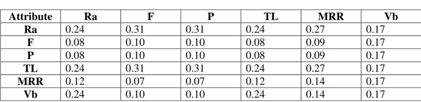
Table 3 shows the performance matrix for various parameters.

Table 3.Performance matrix for various machining parameters [8]

Attribute Ra F P TL MRR Vb Ra 0.24 0.31 0.31 0.24 0.27 0.17 F 0.08 0.10 0.10 0.08 0.09 0.17 P 0.08 0.10 0.10 0.08 0.09 0.17 TL 0.24 0.31 0.31 0.24 0.27 0.17 MRR 0.12 0.07 0.07 0.12 0.14 0.17 Vb 0.24 0.10 0.10 0.24 0.14 0.17 SL. No v f A Ra F P TL MRR Vb 1 30.09 0.12 1.49 0.530 1030.054 5.526 16.866 5261.882 0.096 2 27.33 0.13 1.49 0.560 1115.502 5.416 16.008 5235.061 0.089 3 30.43 0.12 1.49 0.532 1039.400 5.629 16.258 5408.290 0.097 4 26.78 0.13 1.49 0.570 1149.028 5.452 15.454 5321.004 0.088 5 26.77 0.13 1.50 0.563 1129.193 5.366 16.186 5178.547 0.087 6 27.34 0.13 1.48 0.556 1096.056 5.335 16.583 5109.348 0.089 7 29.83 0.12 1.49 0.534 1042.257 5.539 16.597 5296.115 0.095 8 29.82 0.12 1.46 0.535 1027.040 5.470 16.828 5203.697 0.096 9 30.09 0.12 1.45 0.531 1007.984 5.429 17.164 5133.786 0.097 10 30.23 0.12 1.49 0.530 1029.089 5.546 16.782 5287.359 0.096 11 27.44 0.13 1.47 0.556 1087.822 5.321 16.615 5088.652 0.090 12 27.26 0.13 1.48 0.568 1135.683 5.488 15.322 5361.867 0.089 13 30.43 0.12 1.49 0.532 1037.794 5.621 16.320 5395.907 0.097 14 29.80 0.12 1.49 0.540 1062.479 5.625 15.937 5435.633 0.095 15 28.04 0.13 1.49 0.558 1112.254 5.532 15.574 5382.670 0.091 16 06.77 0.14 1.50 0.573 1161.547 5.501 15.123 5399.943 0.087 17 28.39 0.12 1.49 0.542 1067.003 5.397 16.968 5140.209 0.091 18 28.35 0.13 1.49 0.557 1110.184 5.581 15.386 5444.730 0.092 19 27.33 0.13 1.47 0.556 1089.506 5.309 16.655 5074.630 0.089 20 27.44 0.13 1.49 0.560 1113.793 5.428 15.969 5249.625 0.089

B. Tech. Project Report

2014

Mechanical Engineering Department, NIT Rourkela Page 16

SOLUTION

A) PROMETHEE II

By the help of calculated weights and all the above data available for different alternatives and criteria we apply the aforementioned steps of PROMETHEE II to get the rank of all the alternatives. The step by step solution by PROMETHEE II involves a very large number of mathematical calculations so programs in C++ were written for each step and the results of each step were used to determine the final ranking.

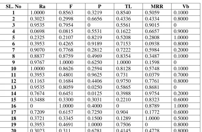
Firstly the performance matrix was normalized by using the formula mentioned in the above step of PROMETHEE II. The normalized matrix obtained is given in Table 4: -

Table 4.Normalized matrix for performance matrix

Thereafter the steps above mentioned in PROMETHEE II are followed to calculate the pairwise difference values and then calculation of preference function is done which is used to determine the weak preference index value and the strong preference index value which are then used to calculate the total preference index. This total preference index is used to obtain the entering flow, the leaving flow and hence the total flow which determines the rank.

SL. No Ra F P TL MRR Vb 1 1.0000 0.8563 0.3219 0.8540 0.5059 0.1000 2 0.3023 0.2998 0.6656 0.4336 0.4334 0.8000 3 0.9535 0.7954 0 0.5561 0.9015 0 4 0.0698 0.0815 0.5531 0.1622 0.6657 0.9000 5 0.2325 0.2107 0.8219 0.5208 0.2808 1.0000 6 0.3953 0.4265 0.9189 0.7153 0.0938 0.8000 7 0.9070 0.7768 0.2812 0.7222 0.5984 0.2000 8 0.8837 0.8759 0.4969 0.8354 0.3487 0.1000 9 0.9767 1.0000 0.6250 1.0000 0.1598 0 10 1.0000 0.8626 0.2594 0.8128 0.5748 0.1000 11 0.3953 0.4801 0.9625 0.731 0.0379 0.7000 12 0.1163 0.1684 0.4406 0.9750 0.7761 0.8000 13 0.9535 0.8059 0.0250 0.5865 0.8681 0 14 0.7674 0.6451 0.0125 0.3988 0.9754 0.2000 15 0.3488 0.3300 0.3031 0.2210 0.8323 0.6000 16 0 1.0000 0.4000 0 0.8789 1.0000 17 0.7209 0.6157 0.7250 0.904 0.1772 0.6000 18 0.3721 0.3345 0.1500 0.1289 1.0000 0.5000 19 0.3953 0.4691 1.0000 0.7506 0 0.8000 20 0.3023 0.311 0.6281 0.4145 0.4728 0.8000

B. Tech. Project Report

2014

Mechanical Engineering Department, NIT Rourkela Page 17

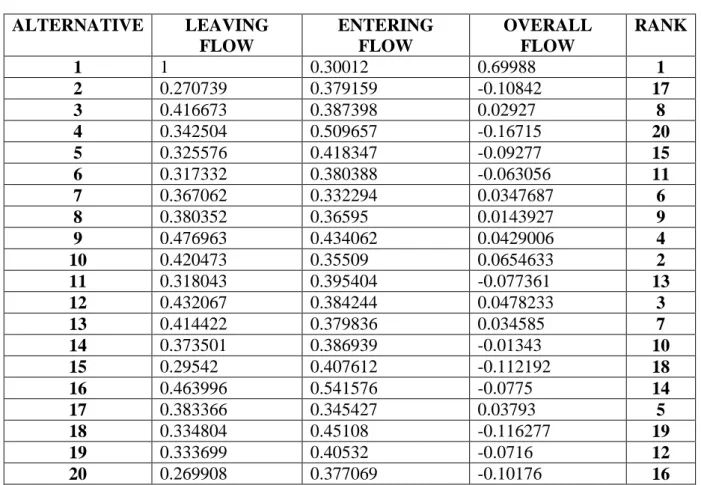
Thus the final ranking obtained by use of PROMETHEE II is shown in Table 5.

Table 5.Overall rank of alternatives ALTERNATIVE LEAVING FLOW ENTERING FLOW OVERALL FLOW RANK 1 1 0.30012 0.69988 1 2 0.270739 0.379159 -0.10842 17 3 0.416673 0.387398 0.02927 8 4 0.342504 0.509657 -0.16715 20 5 0.325576 0.418347 -0.09277 15 6 0.317332 0.380388 -0.063056 11 7 0.367062 0.332294 0.0347687 6 8 0.380352 0.36595 0.0143927 9 9 0.476963 0.434062 0.0429006 4 10 0.420473 0.35509 0.0654633 2 11 0.318043 0.395404 -0.077361 13 12 0.432067 0.384244 0.0478233 3 13 0.414422 0.379836 0.034585 7 14 0.373501 0.386939 -0.01343 10 15 0.29542 0.407612 -0.112192 18 16 0.463996 0.541576 -0.0775 14 17 0.383366 0.345427 0.03793 5 18 0.334804 0.45108 -0.116277 19 19 0.333699 0.40532 -0.0716 12 20 0.269908 0.377069 -0.10176 16

Therefore according to PROMETHEE II the best optimum machining parameters are that of pertaining to Alternative 1.

B) VIKOR

All the steps mentioned above are followed to obtain the best optimum values of cutting speed, feed and depth and rank the other available alternatives according to their performance. Here also the weights calculated by the AHP method are used to calculate the normalized values and also used in the further steps as stated above. The number of calculations is less in comparison to the PROMETHEE II method so there is no requirement of any programme. All the calculations are done by hand and the main values are used in the ranking process. First of all the values are calculated for the required parameters to obtain the rank of the alternatives and these values are used for further steps and calculations.

B. Tech. Project Report

2014

Mechanical Engineering Department, NIT Rourkela Page 18

Table 6.Wj*[(xij)max- xij]/[ (xij)max-( xij)min]

Table 7.Overall rank of alternatives

ALTERNATIVE Ei Fi Pi RANK 1 0.4913 0.2511 0.8969 18 2 05195 0.1427 0.4626 2 3 0.4448 0.2394 0.7909 13 4 0.4791 0.2111 0.7096 11 5 0.5393 0.1551 0.5397 5 6 0.558 0.1551 0.5621 6 7 0.4915 0.2278 0.7966 16 8 0.5085 0.2219 0.7914 14 9 0.5268 0.2453 0.9143 19 10 0.4863 0.2511 0.8909 17 11 0.5563 0.1361 0.4780 3 12 0.4733 0.2274 0.7731 12 13 0.4463 0.2394 0.7927 15 14 0.4444 0.1927 0.5887 7 15 0.4640 0.1963 0.6277 8 16 0.5642 0.2519 0.9874 20 17 0.5489 0.1810 0.6631 9 18 0.4374 0.2195 0.6961 10 19 0.5747 0.1414 0.5229 4 20 0.1561 0.1475 0.0492 1 SL. No Ra F P TL MRR Vb 1 0.2511 0.0858 0.0322 0.0368 0.0699 0.0155 2 0.0759 0.0300 0.0667 0.1427 0.0801 0.1241 3 0.2394 0.0797 0 0.1118 0.0139 0 4 0.0175 0.0082 0.0554 0.2111 0.0473 0.1396 5 0.0584 0.0210 0.0823 0.1207 0.1017 0.1551 6 0.0993 0.0427 0.0921 0.0717 0.01281 0.1241 7 0.2278 0.0778 0.0281 0.0700 0.0568 0.031 8 0.2219 0.0878 0.0497 0.0415 0.0921 0.0155 9 0.2453 0.1001 0.0626 0 0.1188 0 10 0.2511 0.0864 0.026 0.0472 0.0601 0.0155 11 0.0993 0.0481 0.0964 0.0678 0.1361 0.1086 12 0.0292 0.0168 0.0441 0.2274 0.0317 0.1241 13 0.2394 0.0807 0.0033 0.1042 0.0817 0 14 0.1927 0.0646 0.0012 0.1514 0.0035 0.0310 15 0.0876 0.0330 0.0304 0.1963 0.0237 0.0930 16 0 0.1000 0.0400 0.2519 0.0171 0.1551 17 0.1810 0.0617 0.0726 0.0242 0.1164 0.0930 18 0.0934 0.0335 0.0150 0.2195 0 0.0760 19 0.0993 0.0470 0.1001 0.0628 0.1414 0.1241 20 0.0759 0.0312 0.0629 0.1475 0.0745 0.1241

B. Tech. Project Report

2014

Mechanical Engineering Department, NIT Rourkela Page 19

Table 6 is used to tabulate the data calculated by following the first step mentioned in the above process and Table 7 shows the overall rank of the alternatives.

Hence the best alternative according to VIKOR method is Alternative 20.

6.2 Implementation of MCDM methods for selection of a warehouse

Location.

An efficient strategic investment decision is required for the selection of a warehouse location for maximum business profitability. In a business model, one of the important decision making process of the logistic administrators is decision for the location of the distribution centre. After a lot of research a business model with four different alternative warehouses are specified. For the warehouse location, the evaluation criteria are explained as follows in such a way that the criteria based on cost, capacity and customer related to the prospect of sector and business is covered.

 Unit price (UP): It is one of the most important factors in determining the storage of goods in warehouse. If the unit price is less the probability of choosing that location over others increases.

 Stock holding capacity (SHC): This should not be very high which will cause wastage of extra space nor should it be very small. The capacity should be somewhat in the middle level to satisfy this criterion for the decision maker.

 Average distance to shops (ADS): If the presentation period of goods is reduced it provides an important advantage in competition for retail sector businesses. The main aim of a decision maker should always be to choose such a location which will provide the company a good access to the shops when they run out of products from their rival business. If the distance to shops is less it will be in the advantage of the company.

 Average distance to main suppliers (ADM): Minimizing this criterion will also help in good business for the company.

 Movement flexibility (MF): The movement flexibility is decided by the evaluation of architectural and layout factors of the warehouse location which tells about the total storage space in the warehouse and other conformity factors. Thus alternative warehouse locations are evaluated based on 0-4 scale (really bad, bad, average, good and really good).

So the beneficial attributes (higher is better) are stock holding capacity and movement flexibility and the non-beneficial attributes are unit price, average distance to shops and average distance to main suppliers. Table 8 shows all the attributes pertaining to different criteria.

The importance weights of criteria in the decision problem are, {WUP, WSHC, WADS, WADM,

B. Tech. Project Report

2014

Mechanical Engineering Department, NIT Rourkela Page 20

Table 8.Performance values of warehouse alternatives [9] ALTERNATIVE Unit price

($/m2) Stock holding capacity (unit) Average distance to shops (kilometre) Average distance to main suppliers (kilometre) Movement flexibility A 7 100 20 14 3 B 10 120 8 10 1 C 8 150 12 12 2 D 6 180 16 13 4

SOLUTION

A) PROMETHEE II

By the help of calculated weights and all the above data available for different alternatives and criteria we apply the aforementioned steps of PROMETHEE II to get the rank of all the alternatives.

Again the normalized matrix was calculated by the aforementioned formula and tabulated in Table 9.

Table 9.Normalized matrix

ALTERNATIVE UP SHC ADS ADM MF

A 0.75 0 0 0 0.67

B 0 0.25 1.00 1.00 0

C 0.50 0.63 0.67 0.50 0.33

D 1.00 1.00 0.33 0.25 1.00 Thus the final ranking obtained by use of PROMETHEE II is shown in Table 10.

Table 10.Overall rank of alternatives ALTERNATIVE LEAVING FLOW ENTERING FLOW OVERALL FLOW RANK A 0.348533 0.759683 -0.41115 4 B 0.488333 0.723917 -0.235583 3 C 0.498267 0.37695 0.121317 2 D 0.82425 0.298833 0.525417 1

B. Tech. Project Report

2014

Mechanical Engineering Department, NIT Rourkela Page 21

B) VIKOR

All the steps mentioned above are followed to obtain the best warehouse location. Here also the weights calculated by the AHP method are used to calculate the normalized values and also used in the further steps as stated above. Table 11 is used to tabulate the data calculated by following the first step mentioned in the above process.

Table 11.Wj*[(xij)max- xij]/[ (xij)max-( xij)min]

ALTERNATIVE UP SHC ADS ADM MF

A 0.2175 0 0 0 0.402

B 0 0.8750 0.1500 0.1500 0

C 0.1450 0.2190 0.1000 0.0500 0.1980

D 0.2900 0.3500 0.0500 0.3750 0.0600

After calculating this further steps are followed and the final rank is tabulated in Table 12.

Table 12.Overall rank of alternatives

ALTERNATIVE Ei Fi Pi RANK

1 0.2577 0.402 0.1396 1 2 0.3875 0.875 0.6226 4 3 0.55905 0.2188 0.2847 2 4 0.7870 0.375 0.6190 3

6.3 Cutting tool material selection using PROMETHEE II and VIKOR

methods.

In this modern era of metal working industry, a series of materials, like high speed steel, ceramic materials, diamond, carbide tool etc. are used as cutting tools. Because of a variety of conditions and requirements, for all the machining applications, a single cutting tool cannot be used. Each and every cutting tool material has its own characteristics and properties that make it best for a specific machining application. For selection of a cutting tool material it is important to go through all the physical properties of the material available. Thus, it is always desirable that the most appropriate cutting tool material for a specific application with the desired physical properties for high machining performance be selected. Here a list of 19 cutting tool materials has been made which are to be chosen on the basis of 10 different criterions.

B. Tech. Project Report

2014

Mechanical Engineering Department, NIT Rourkela Page 22

Table 13.Cutting tool material selection criteria [10] Properties of cutting tool materials

(criteria)

Symbol

Density (gm/cc) C1

Hardness (HK) C2

Yield tensile strength (MPa) C3

Modulus of elasticity (GPa) C4

Compressive strength (MPa) C5

Shear strength (MPa) C6

Charpy impact strength (J) C7

Thermal conductivity (W/mK) C8

Coefficient of linear thermal expansion (µm/m-°C)

C9

Tool material cost (USD/kg) C10

Table 13 shows different criteria and their symbols.

Table 14.Cutting tool material alternatives [10] Cutting tool materials Symbol

Powder metal tool steel (AISI A11) A1

Oil quenched tool steel (AISI O2) A2

Cobalt-free super high speed steel A3

Air-hardened tool steel (ASTM A2) A4

Tool steel (ASTM A6) A5

Shock-resisting tool steel (ASTM S7) A6

Tungsten-molybdenum high speed steel (W-Mo)

A7

Sintered reaction bonded silicon nitride A8

Titanium carbide A9

Cermet A10

Tungsten carbide A11

Mono-tungsten carbide A12

Stellite (cast cobalt alloy) A13

Sialon A14

Cubic boron nitride (CBN) A15

Alumina (99.9% pure) A16

Synthetic polycrystal diamond A17

Synthetic single crystal diamond A18

Hot pressed silicon nitride A19

Table 14 tabulates various alternatives available and their symbols.

B. Tech. Project Report

2014

Mechanical Engineering Department, NIT Rourkela Page 23

Table 15.Decision matrix for cutting tool material [10]

SL. No C1 C2 C3 C4 C5 C6 C7 C8 C9 C10 A1 7.40 754 1975 220 2190 1684 65.00 22.00 11.40 1.65 A2 7.61 624 1751 140 1890 1492 105.00 39.00 10.30 1.25 A3 8.17 908 2228 235 3145 1899 18.00 46.00 10.67 9.70 A4 7.86 822 2090 207 2357 1782 678.00 26.00 14.00 1.90 A5 7.83 788 2012 207 2200 1715 407.00 14.70 13.01 5.30 A6 7.83 677 1874 207 1976 1597 16.90 28.50 12.40 2.15 A7 8.14 826 2065 208 3000 1760 23.00 37.00 11.30 10.85 A8 3.30 2550 128 310 1035 410 0.10 42.00 3.10 400.00 A9 4.94 1800 237 451 3475 756 1.24 17.00 7.70 18.00 A10 14.95 1276 1324 600 6150 4219 1.35 60.00 4.60 78.60 A11 15.00 1387 415 690 4975 1324 1.34 98.00 6.50 60.00 A12 15.70 1167 316 696 2683 1008 1.27 82.00 5.20 65.00 A13 8.77 803 379 243 2300 1210 1.25 8.40 11.47 87.50 A14 3.25 1959 381 345 3450 1216 1.07 19.00 3.50 557.00 A15 8.60 5000 481 850 6900 1532 0.50 13.00 4.80 864.00 A16 9.36 1700 276 370 3000 879 0.10 30.00 5.43 152.12 A17 4.00 7000 1472 953 6700 4688 0.10 1200 3.80 1300.00 A18 3.80 8000 1794 1050 6900 5713 0.20 1500 4.80 1500.00 A19 3.20 2730 501 310 3450 1612 .012 39 10.71 337.00

The weights of different criterions are {W1, W2, W3, W4, W5, W6, W7, W8, W9, W10} =

{0.0232, 0.0716, 0.0549, 0.038, 0.0248, 0.0424, 0.2227, 0.2939, 0.0212, 0.2023}.

SOLUTION

A) PROMETHEE II

By the help of calculated weights and all the above data available for different alternatives and criteria we apply the aforementioned steps of PROMETHEE II to get the rank of all the alternatives. Table 16 shows the normalized matrix values.

B. Tech. Project Report

2014

Mechanical Engineering Department, NIT Rourkela Page 24

Table 16.Normalized matrix of the decision matrix

SL. No C1 C2 C3 C4 C5 C6 C7 C8 C9 C10 A1 0.3360 0.0176 0.8795 0.0879 0.1969 0.2400 0.6187 0.0091 0.2385 0.9997 A2 0.3530 0 0.7729 0 0.1458 0.2040 1.0000 0.0205 0.3394 1.0000 A3 0.3970 0.0385 1.0000 0.1044 0.3598 0.2130 0.1706 0.0252 0.3055 0.9944 A4 0.3728 0.0268 0.9343 0.0736 0.2254 0.2587 0.6454 0.0118 0 0.9996 A5 0.3704 0.0222 0.8971 0.0736 0.1604 0.2238 0.1602 0.0134 0.1468 0.9973 A6 0.3704 0.0072 08314 0.0736 0.1604 0.2238 0.1602 0.0134 0.1468 0.9994 A7 0.3952 0.0274 0.9224 0.0747 0.3350 0.2546 0.2183 0.0192 0.2477 0.9936 A8 0.0008 0.2611 0 0.1868 0 0 0 0.0225 1.0000 0.7339 A9 0.1392 0.1594 0.0519 0.3418 0.4160 0.0652 0.0109 0.0058 0.578 0.9888 A10 0.9400 0.0884 0.5695 0.5056 0.8721 0.7183 0.0119 0.0346 0.8624 0.9484 A11 0.9440 0.1034 0.1367 0.6044 0.6718 0.1724 0.0118 0.0601 0.6881 0.9608 A12 1.0000 0.0736 0.0895 0.6110 0.2810 0.1128 0.0012 0.0493 0.8073 0.9575 A13 0.4456 0.0247 0.1195 0.1132 0.2157 0.1508 0.0092 0 0.2321 0.9425 A14 0.0040 0.1810 0.1205 0.2253 0.4118 0.1519 0.0038 0.0071 0.9630 0.6291 A15 0.4320 0.5934 0.1681 0.7802 1.0000 0.2116 0.0004 0.0031 0.8440 0.4243 A16 0.4928 0.1459 0.0705 0.2527 0.3350 0.0884 0 0.0145 0.7862 0.8993 A17 0.0640 0.8644 0.6400 0.8934 0.9659 0.8067 0 0.7989 0.9358 0.1334 A18 0.0480 1.0000 0.7933 1.0000 1.0000 1.0000 0.0009 1.0000 0.8440 0 A19 0 0.2855 0.1800 0.1868 0.4118 0.2267 0.0002 0.0205 0.3018 0.7760

After following all the steps of the method we get the final ranking as shown in Table 17. Table 17.Overall rank of alternatives

ALTERNATIVE LEAVING FLOW

ENTERING FLOW

NET FLOW RANK A1 0.1444222 0.0846284 0.059735 5 A2 0.2257 0.084145 0.141555 3 A3 0.072532 0.0947689 -0.0222369 9 A4 0.153508 .0861185 0.0673895 4 A5 0.098929 0.0966934 0.00223649 6 A6 0.0548962 0.108657 -0.0537605 13 A7 0.0729946 0.0956567 -0.0226621 10 A8 0.281694 0.149718 -0.121549 18 A9 0.241383 0.034107 -0.109969 17 A10 0.8857510 0.922679 -0.0036928 7 A11 0.0613371 0.0110261 -0.0489236 12 A12 0.0522038 0.118428 -0.0066245 8 A13 0.011451 0.1424 -0.130949 19 A14 0.0256708 0.134462 -0.0108791 16 A15 0.083299 0.114256 -0.0309651 11 A16 0.0258236 0.128918 -0.103094 14 A17 0.355548 0.0733479 0.2822 2 A18 0.441397 0.0682254 0.373171 1 A19 0.0272658 0.130803 -0.103537 15

B. Tech. Project Report

2014

Mechanical Engineering Department, NIT Rourkela Page 25

B) VIKOR

All the steps mentioned above are followed to obtain the best cutting tool material. Here also the weights calculated by the AHP method are used. Since the number of calculations are less no programming is required. Table 18 is used to tabulate the data calculated by following the first step mentioned in the above process.

Table 18.Wj*[(xij)max- xij]/[ (xij)max-( xij)min]

SL. No C1 C2 C3 C4 C5 C6 C7 C8 C9 C10 A1 0.0079 0.0013 0.0483 0.0034 0.0049 0.0102 0.1378 0.0027 0.0051 0.2022 A2 0.0082 0 0.0424 0 0.0036 0.0086 0.2227 0.0060 0.0072 0.2023 A3 0.0092 0.0029 0.0549 0.0039 0.0089 0.0119 0.0380 0.0074 0 0.2022 A4 0.0086 0.0017 0.0493 0.0028 0.0056 0.0190 0.1437 0.0035 0 0.2022 A5 0.0086 0.0017 0.0493 0.0028 0.0049 0.0104 0.0862 0.0012 0.0018 0.2018 A6 0.0086 0.0005 0.0456 0.0028 0.0040 0.0095 0.0357 0.0039 0.0031 0.2022 A7 0.0092 0.0021 0.0506 0.0028 0.0083 0.0107 0.0486 0.0056 0.0053 0.2010 A8 0 0.0200 0 0.0071 0 0 0 0.0066 0.0212 0.1485 A9 0.0032 0.0122 0.0028 0.0129 0.0103 0.0028 0.0024 0.0017 0.0123 0.2000 A10 0.0218 0.0068 0.0313 0.0192 0.0216 0.0305 0.0026 0.0102 0.0183 0.1919 A11 0.0219 0.0079 0.0075 0.0230 0.0167 0.0073 0.0026 0.0177 0.0146 0.1937 A12 0.0232 0.0056 0.0049 0.0232 0.0070 0.0048 0.0025 0.0145 0.0171 0.1937 A13 0.0103 0.0018 0.0016 0.0043 0.0064 0.0020 0 0.0049 0 0.1907 A14 0 0.0456 0.0092 0.0296 0.0248 0.0064 0 0.0009 0.0204 0.1273 A15 0.0100 0.0456 0.0092 0.0296 0.0248 0.0089 0 0.0009 0.0179 0.0858 A16 0.0114 0.0112 0.0039 0.0096 0.0083 0.0003 0 0.0042 0.0167 0.1819 A17 0.0015 0.0662 0.0351 0.0339 0.0239 0.0342 0 0.2348 0.0198 0.0269 A18 0.0011 0.0716 0.0435 0.0380 0.0248 0.0424 0 0.2939 0.0179 0 A19 0 0.0219 0.0099 0.0071 0.0102 0.0096 0 0.0060 0.0064 0.1570

B. Tech. Project Report

2014

Mechanical Engineering Department, NIT Rourkela Page 26

Table 19. Overall rank of alternatives

ALTERNATIVE Ei Fi Pi RANK A1 0.4238 0.2022 0.0587 1 A2 0.5010 0.2227 0.1185 5 A3 0.3448 0.2012 0.5040 17 A4 0.3015 0.2022 0.4453 12 A5 0.3687 0.2018 0.5392 18 A6 0.3159 0.2022 0.4656 13 A7 0.3442 0.2010 0.5027 15 A8 0.2034 0.1485 0.1776 6 A9 0.2606 0.2000 0.3882 10 A10 0.3605 0.1919 0.5039 16 A11 0.3370 0.1944 0.4768 14 A12 0.2965 0.1937 0.4178 11 A13 0.1843 0.1907 0.2520 8 A14 0.1963 0.1273 0.1167 4 A15 0.2327 0.0858 0.0684 2 A16 0.2475 0.1819 0.3202 9 A17 0.4763 0.2348 0.7705 19 A18 0.5382 0.2939 0.1000 3 A19 0.2272 0.1570 0.2317 7

Table 19 is used to tabulate the overall rank of the available alternatives and it is found that the best alternative is A1.

B. Tech. Project Report

2014

Mechanical Engineering Department, NIT Rourkela Page 27

6.4 Use of a MCDM approach for selection of suppliers in auto industry

In selection of a supplier various criterions are to taken into account, so we require a MCDM approach to determine which supplier will meet our requirements best according to the criteria values set by us. Here we encounter various issues related to supplier selection in an auto industry. The various criteria involved in decision making process are: -

 (C1) PPM (Part per million) customers: It measures the number of parts returned per

million by the customer.

 (C2) Quality: The quality of goods provided by the suppliers.

 (C3) Price/ cost: The cost which the enterprise pays for the goods.

 (C4) Standardization: The extent of pre-set standards followed by the company during

the manufacturing process.

 (C5) Service: The support and service provided by a supplier after sales of the

product.

 (C6) Flexibility: The extent to which the supplier is able to cope up with the change in

demand of the customer.

 (C7) On time delivery: The time taken by the supplier to supply the parts.

Here the criteria C1 and C3 are non-beneficial and the attributes pertaining to other criteria are

beneficial.

The weight calculated by AHP method are {W1, W2, W3, W4, W5, W6, W7} = {0.376, 0.155,

0.062, 0.208, 0.059, 0.037, 0 .099}.

Table 20.Performance matrix of alternatives [11]

ALTERNATIVE C1 C2 C3 C4 C5 C6 C7

S1 0.475 0.435 0.479 0.542 0.379 0.571 0.600

S2 0.425 0.446 0.524 0.475 0.525 0.452 0.585

S3 0.552 0.543 0.325 0.313 0.500 0.452 0.432

S4 0.535 0.396 0.465 0.570 0.422 0.356 0.596

The performance matrix of alternatives is tabulated in Table 20.

SOLUTION

A) PROMETHEE II

By the help of calculated weights and all the above data available for different alternatives and criteria we apply the aforementioned steps of PROMETHEE II to get the rank of all the alternatives.

B. Tech. Project Report

2014

Mechanical Engineering Department, NIT Rourkela Page 28

The normalized values are first calculated and tabulated in Table 21.

Table 21.Normalization matrix

ALTERNATIVE C1 C2 C3 C4 C5 C6 C7

S1 0.606 0.265 0.226 0.891 0 1.000 1.000

S2 1.000 0.340 0 0.630 1.000 0.446 0.912

S3 0 1.000 1.000 0 0.829 0.446 0

S4 0.134 0 0.307 1.000 0.294 0 0.976

Overall rank of the alternatives after various calculations is tabulated in Table 22 which shows the best alternative is S1.

Table 22.Overall rank of alternatives ALTERNATIVE LEAVING FLOW ENTERING FLOW OVERALL FLOW RANK S1 0.602977 0.410119 0.192585 1 S2 0.623036 0.59021 0.032826 3 S3 0.61489 1 -0.38511 4 S4 0.639329 0.479903 0.159425 2

B) VIKOR

All the steps mentioned above are followed to obtain the best cutting tool material. Table 23 is used to tabulate the data calculated by following the first step mentioned in the above process.

Table 23.Wj*[(xij)max- xij]/[ (xij)max-( xij)min]

Table 24.Overall rank of alternatives

Table 24 clearly shows that S3 is the best alternative available by this process.

ALTERNATIVE C1 C2 C3 C4 C5 C6 C7 S1 0.228 0.041 0.014 0.185 0 0.037 0.099 S2 0.376 0.053 0 0.131 0.059 0.017 0.090 S3 0 0.155 0.062 0 0.049 0.017 0 S4 0.050 0 0.019 0.208 0.017 0 0.097 ALTERNATIVE Ei Fi Pi RANK S1 0.604 0.228 0.527 3 S2 0.726 0.376 1.000 4 S3 0.283 0.155 0 1 S4 0.391 0.208 0.242 2

B. Tech. Project Report

2014

Mechanical Engineering Department, NIT Rourkela Page 29

7. Conclusion

This thesis explains the two MCDM methods namely PROMETHEE II and VIKOR clearly and the solution of four engineering problems from different fields gives a clear cut idea on the diverse applications of these two MCDM methods. Both methods follow different algorithm so the results obtained by both algorithms are different.

B. Tech. Project Report

2014

Mechanical Engineering Department, NIT Rourkela Page 30

8. Bibliography

1) http://en.wikipedia.org/wiki/Multiple-criteria_decision_analysis.

2) N. Patel, 2013, “A comparative analysis of TOPSIS & VIKOR methods in the selection of industrial robots”, B. Tech thesis, NIT Rourkela.

3) A. Chauhan, R. Vaish, 2012, “Hard coating material selection using multi-criteria decision making”, Materials and design, 44, pp. 240–245.

4) H. Çalıskan, 2013, “Selection of boron based tribological hard coatings using multi-criteria decision making methods”, Materials and design, 50, pp. 742–749.

5) J. Ren, A. Fedele, M. Mason, A. Manzardo, 2013, “Fuzzy multi-factor multi-criteria decision making for sustainability assessment of biomass-based technologies for hydrogen production”, International journal of hydrogen energy, 38, pp. 9111-9120.

6) M.A. Keramati, M. Khezerloo, M. Golbaharzadeh, 2013, “Ranking of manufacturers of mechanical parts based on a fuzzy multi-criteria decision making method: a case study in Iran national steel industrial group”, European online journal of natural and social sciences, 2, pp. 672-685.

7) P. Adhikary, S. Kundu, 2014, “MCDA or MCDM based selection of transmission line conductor: small hydropower project planning and development”, International journal of engineering research and applications, 4, pp. 357-361.

8) R. Thirumalai, J. S. Senthilkumaar, 2012, “Multi-criteria decision making in the selection of machining parameters for Inconel 718”, Journal of mechanical science and technology, 27, pp. 1109-1116.

9) T. Özcan, N. Çelebi, S. Esnaf, 2011, “Comparative analysis of multi-criteria decision making methodologies and implementation of a warehouse location selection problem”, Expert systems with applications, 38, pp. 9773–9779.

10) S.R. Maity, P. Chatterjee, S. Chakraborty, 2012, “Cutting tool material selection using grey complex proportional assessment method”, Materials and design, 36, pp. 372–378. 11) K. Shahroudi, H. Rouydel, 2012, “Using a multi-criteria decision making approach (ANP-TOPSIS) to evaluate suppliers in Iran’s auto industry”, International journal of applied operational research, 2(2), pp. 37-48.

12) T. L. Satty. The analytic hierarchy process. McGraw-Hill: New York; 1980.

13) G.H. Tzeng, J.J. Huang. Multiple attribute decision making: methods and applications. CRC Press: USA; 2011.

B. Tech. Project Report

2014

Mechanical Engineering Department, NIT Rourkela Page 31

14) N.Hamidi, P.M. Pezeshki, A. Moradian, 2010, “Weighting the criteria of brand selecting in beverage industries in Iran”, Asian journal of management research, 12, pp. 250–267. 15) P. Chatterjee, S. Chakraborty, 2012, “Material selection using preferential ranking methods”, Material and design, 35, pp. 384–393.

16) M. Doumpos, C. Zopounidis, 2004, “A multi-criteria classification approach based on pairwise comparisons”, European journal operation research, 158, pp. 378–389.

17) K.S. Raju, D.N. Kumar, 1999, “Multi-criterion decision making in irrigation planning”, Agricultural system, 62, pp. 117–129.

18) H. Çalıskan, B. Kursuncu, C. Kurbanoglu, S.Y. Güven, 2013, “Material selection for the tool holder working under hard milling conditions using different multi criteria decision making methods”, Materials and design, 45, pp. 473–479.