Noname manuscript No.
(will be inserted by the editor)
Spatial-Temporal modellization of the NO
2concentration data through
geostatistical tools
Raquel Menezes⇤a, Helena Piairoa, Pilar Garc´ıa-Soid´anb, Inˆes Sousaa
Received: date / Accepted: date
Abstract The nitrogen dioxide is a primary pollutant, regarded for the estimation of the air quality index, whose excessive presence may cause significant environmental and health problems. In the current work, we suggest characterizing the evolution of NO2levels, by using
geostatisti-cal approaches that deal with both the space and time coordinates. To develop our proposal, a first exploratory analysis was carried out on daily values of the target variable, daily measured in Portugal from 2004 to 2012, which led to identify three influential covariates (type of site, environment and month of measurement). In a second step, appropriate geostatistical tools were applied to model the trend and the space-time variability, thus enabling us to use the kriging techniques for prediction, without requiring data from a dense monitoring network. This method-ology has valuable applications, as it can provide accurate assessment of the nitrogen dioxide concentrations at sites where either data have been lost or there is no monitoring station nearby.
Keywords NO2·Geostatistics·Time series analysis·Space-time analysis
aCentre of Mathematics, University of Minho, Campus of Azurem, 4800-058 Guimar˜aes, Portugal bDepartment of Statistics and O.R., University of Vigo, Campus of A Xunqueira, Pontevedra 36005, Spain ⇤Corresponding author: [email protected], phone +351 253510400 / fax +351 253510400
Noname manuscript No. (will be inserted by the editor)
Spatial-Temporal modellization of the NO
2concentration data through
geostatistical tools
Received: date / Accepted: date
Abstract The nitrogen dioxide is a primary pollutant, regarded for the estimation of the air quality index, whose excessive presence may cause significant environmental and health problems. In the current work, we suggest characterizing the evolution of NO2levels, by using geostatisti-cal approaches that deal with both the space and time coordinates. To develop our proposal, a first exploratory analysis was carried out on daily values of the target variable, daily measured in Portugal from 2004 to 2012, which led to identify three influential covariates (type of site, environment and month of measurement). In a second step, appropriate geostatistical tools were applied to model the trend and the space-time variability, thus enabling us to use the kriging techniques for prediction, without requiring data from a dense monitoring network. This method-ology has valuable applications, as it can provide accurate assessment of the nitrogen dioxide concentrations at sites where either data have been lost or there is no monitoring station nearby. Keywords NO2·Geostatistics·Time series analysis·Space-time analysis
1 Introduction
The air quality is the term usually coined to refer to the degree of pollution in the air that we breathe. The air pollution may be caused by a mixture of chemical elements released into the air or by chemical reactions that change the natural constitution of the atmosphere WHO (2003). These pollutants may have a greater or lesser impact on the air quality, depending on their chemical composition, their concentration in air and the weather conditions. Among the number of problems derived from the air pollution, we can mention the degradation of air quality, the human and ecosystem exposure to toxic substances, the damage in built heritage, the deterioration of the stratospheric ozone layer or the global warming/climate change.
Estimation of the index of air quality involves measurements of the following chemical ele-ments: carbon monoxide (CO), nitrogen dioxide (NO2), sulphur dioxide (SO2), ozone (O3) and fine particulate matter as PM10. Regarding the aforementioned pollutants, we aim to study NO2 concentrations, because of its presence in urban and industrial areas. NO2 is considered a pri-mary pollutant, which may be produced by emissions from electricity generating stations, heavy industry and road transport, as well as the burning of biomass. However, the nitrogen oxides can also be naturally produced by the lightning or the microbial activity in the soil (Carslaw, 2005). 1 2 3 4 5 6 7 8 9 10 11 12 13 14 15 16 17 18 19 20 21 22 23 24 25 26 27 28 29 30 31 32 33 34 35 36 37 38 39 40 41 42 43 44 45 46 47 48 49 50 51 52 53 54 55
The EU legislation regarding environmental pollution was recently revised to incorporate the latest scientific and technical developments, yielding the publication of the Directive 2008/50/EC on ambient air quality and cleaner air for Europe. The concentrations of NO2have been analyzed extensively in many urban areas in European cities (Stedman et al, 2001; Lewne et al, 2004; Carslaw, 2005; Lindley and Walsh, 2005; Grice et al, 2009). Several of these studies have shown that NOx emissions, and subsequently NOx concentrations, have been reduced in Europe, in compliance with the EU standards and directives; however, this has not yielded a corresponding reduction of NO2concentrations in ambient.
The current research is focused on providing a procedure to characterize the spatial and temporal evolution of the nitrogen dioxide levels through the use of geostatistical approaches. In particular, our proposal will be applied to the data set collected in Portugal from 2004 to 2012. To have a preliminary overview, a simple analysis will be first derived to obtain the summary statistics for each year as well as for the whole data set. We will also deal with di↵erent factors that can be associated to the concentrations of NO2measured at each of the monitored locations, such as the type of site or the environment of the zone, referred to in the European Directive, as well as the time of the year when the data are collected. The resulting significative covariates will be considered in a second step, where we will address the trend estimation of the NO2data and the characterization of the space-time variability of the residuals, through geostatistical approaches. The subsequent application of the kriging techniques will enable us to reconstruct the space-time pattern followed by the NO2concentrations together with the associated prediction error. As we will give account, this methodology can be particularly useful to ensure adequate assessment of the target variable at a specific site where there is no monitoring station nearby or data have been lost, due to the regular calibration and maintenance of its instrumentation or another reason.
This paper is organized as follows. Section 2 describes the monitoring network and the data set used to derive the analysis of the NO2 concentrations at the monitored sites, as well as the results of the preliminary study. We present in Section 3 a brief review of the spatio-temporal methodology, paying special attention to the geostatistical approaches that will be applied to the nitrogen dioxide values. Section 4 discusses the results achieved for the di↵erent issues (estimation of the trend, structural analysis and kriging prediction), together with some applications of the current research. The main conclusions are summarized in Section 5.
2 The portuguese monitoring network 2.1 Source of data
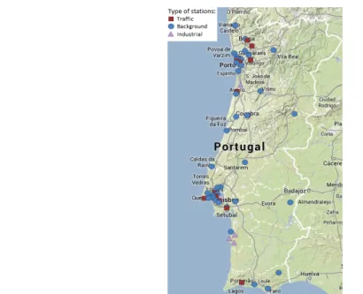
The ambient air quality has been the subject of extensive work by the governments and re-searchers from di↵erent countries. This aim has been developed in Portugal for the Ministry of Environment, Spatial Planning and Energy, under the Portuguese Environment Agency, in as-sociation with the North Regional Coordination and Development Commission in Portugal and the Environmental Departments of the Autonomous Regions. In addition, a system of monitor-ing air quality was promoted by the Portuguese Environment Agency to fulfill the requirements established in the aforementioned directive. The air pollution in Portugal is determined from the data collected in various monitoring stations located predominantly in large urban areas (with heavy traffic) or the most relevant industrial areas, as shown in Fig. 1.
The monitoring stations report hourly concentrations of various chemical elements and, par-ticularly, of NO2, which is a critical pollutant. The available data include the hourly measure-ments at the di↵erent locations as well as information of other factors, mentioned in the EU legislation, such as the type of site where the station is placed (background, industrial and traf-fic) and the environment of the zone (urban, suburban and rural). A total of 88 monitoring sites
2 3 4 5 6 7 8 9 10 11 12 13 14 15 16 17 18 19 20 21 22 23 24 25 26 27 28 29 30 31 32 33 34 35 36 37 38 39 40 41 42 43 44 45 46 47 48 49 50 51 52 53 54 55
Fig. 1 Location and type of site of the stations in the area studied (Portugal).
were used in the analysis (47 background, 34 traffic and 7 industrial sites), where 60 of them were located in urban areas, 14 in suburban areas and 14 in rural areas. Further details on this data set can be found in QualAr (qualar.apambiente.pt/).
2.2 Preliminary data analysis
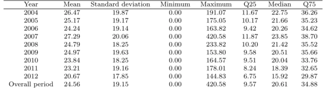
The data analysis was carried out to characterize the evolution of NO2 levels in Portugal from 2004-2012. In our study, we considered daily averages of the nitrogen dioxide concentration values, since the application of the geostatistical methodology on the original data set, corresponding to the hourly measurements in the period 2004-2012 at the 88 monitoring sites, would be too computationally expensive. In addition, a nine-year period is considered, as this research aims at capturing the annual seasonality inherent in this kind of data. Table 1 gives the summary statistics, showing that the mean and median values of the NO2 data decrease in the period 2004-2012, except for 2007. We should notice that during these years there was an increasing concern about the environment in Portugal that remains nowadays. Some outliers were observed in the years 2007 and 2008, with respective maxima of 420.58 and 233.82 µg/m3, which were removed from the data for the spatio-temporal analysis.
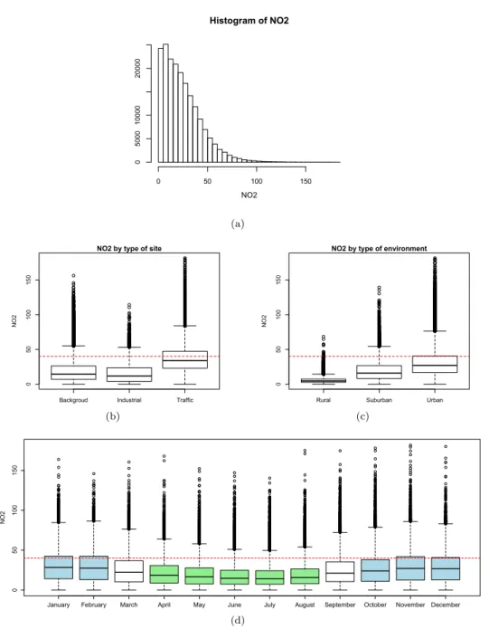
The daily averages of NO2concentrations are represented in Fig. 2(a), giving account of its asymmetric distribution. We will bear in mind this feature for addressing the estimation of the trend of the underlying process. On the other hand, Fig. 2(b)-(d) depict boxplots obtained for the daily values of NO2, portraying the di↵erences by type of site, type of environment and month. The influence of the location can be observed in Fig. 2(b), so that the stations located at background or industrial areas show a similar behavior, attaining significant smaller values for their quartiles than those derived for traffic areas. With regard to the environment, a substantial increment on the NO2 concentrations is observed, when we move from the rural to the urban zones, as shown in Fig. 2(c). In addition, the daily averages present in Fig. 2(d) di↵erent patterns 2 3 4 5 6 7 8 9 10 11 12 13 14 15 16 17 18 19 20 21 22 23 24 25 26 27 28 29 30 31 32 33 34 35 36 37 38 39 40 41 42 43 44 45 46 47 48 49 50 51 52 53 54 55
Table 1 Descriptive statistics obtained for the daily averages of NO2concentrations (µg/m3).
Year Mean Standard deviation Minimum Maximum Q25 Median Q75 2004 26.47 19.87 0.00 191.07 11.67 22.75 36.26 2005 25.17 19.17 0.00 175.05 10.17 21.66 35.23 2006 24.24 19.14 0.00 163.82 9.42 20.26 34.62 2007 27.29 20.06 0.00 420.58 11.87 23.85 38.70 2008 24.79 18.25 0.00 233.82 10.20 21.42 35.52 2009 24.97 19.63 0.00 153.80 9.58 20.51 35.66 2010 23.84 18.25 0.00 164.57 9.51 20.04 33.76 2011 23.21 19.16 0.00 178.01 8.24 18.39 32.65 2012 20.67 17.85 0.00 144.83 6.75 15.92 29.87 Overall period 24.56 19.15 0.00 420.58 9.57 20.61 34.88
for the central months (from April to August) with respect to the rest of the year, achieving the highest and the lowest values in the winter and summer periods, respectively, as in Saiz-Lopez et al (2009). The latter gives account of the existence of a seasonal e↵ect in the data set. Some studies (Heuvelink and Griffith, 2010) exclude the seasonal component from the analysis, whereas others (De Iaco and Posa, 2012) include this e↵ect either into the trend estimation or into the space-time variogram.
3 Methodology
The spatial and temporal variability is often used to characterize the performance of environmen-tal processes, such as atmospheric pollutant concentrations, precipitation fields or surface winds. This tool enables the researchers to develop statistical models, continuous in space and time and based on observations at a limited number of monitoring stations, which are computationally less expensive than those strategies requiring data from a dense monitoring network (Gneiting et al, 2007, Chapter 4).
Consider a random function Z(s, t) : (s, t)2Rd⇥R , indexed in space by s 2Rd and in time by t 2 R. The application of the spatio-temporal geostatistical tools demands assuming that the target variable is random at each location s and time t. However, no more than a single realization of the random variableZ(s, t) is available at each (s, t), thus leading to require additional hypotheses on the data setting to make inference possible, such as stationarity or isotropy. The stationarity condition can be relaxed by admitting the following decomposition for the random process:
Z(s, t) =µ(s, t) +"(s, t) (1)
whereµ(·) denotes the trend and"(·) is a zero-mean stationary residual.
Under model (1), we must start by characterizing the trend, which can be addressed by assuming that it is either a deterministic or a random variable (Kyriakidis and Journel, 1999). In the latter case, specific approaches for the space-time setting can be applied (Host et al, 1995) or more common alternatives, such as that based on the generalized regression procedure (Goovaerts, 1997). For estimation of a deterministic trend, di↵erent forms to model complex settings have been proposed (Dimitrakopoulos and Luo, 1997), which can even incorporate the seasonal e↵ect. Additional options to accomplish specification of the trend can be derived through broad-spectrum approaches, as the generalized linear estimation (Fox, 2008) or the median polish algorithm (Bruno et al, 2009). We should highlight that both assumptions for the trend can provide similar predictions, when the dependence structure of the residual data is appropriately characterized (De Iaco and Posa, 2012).
2 3 4 5 6 7 8 9 10 11 12 13 14 15 16 17 18 19 20 21 22 23 24 25 26 27 28 29 30 31 32 33 34 35 36 37 38 39 40 41 42 43 44 45 46 47 48 49 50 51 52 53 54 55
Histogram of NO2 NO2 0 50 100 150 0 5000 10000 20000 (a)
Backgroud Industrial Traffic
0
50
100
150
NO2 by type of site
NO2
(b)
Rural Suburban Urban
0
50
100
150
NO2 by type of environment
NO2
(c)
January February March April May June July August September October November December
0 50 100 150 NO2 (d)
Fig. 2 A histogram of the daily averages of NO2concentrations is displayed in Fig. 2(a)). The remainder panels
represent boxplots of the daily averages of NO2concentrations in the period 2004-2012, by type of site (Fig. 2(b)),
by type of environment (Fig. 2(c)) and by month (Fig. 2(d)). In all boxplots, the red dashed-line represents the annual mean limit of 40µg/m3.
The hierarchical statistical methods can also be applied in the spatio-temporal setting (Cressie and Wikle, 2011), by proceeding through conditional-probability modeling and by considering di↵erent levels for specification of the unknown terms involved (Shaddick et al, 2013). These
2 3 4 5 6 7 8 9 10 11 12 13 14 15 16 17 18 19 20 21 22 23 24 25 26 27 28 29 30 31 32 33 34 35 36 37 38 39 40 41 42 43 44 45 46 47 48 49 50 51 52 53 54 55
approaches can incorporate latent processes or temporal dynamics (Cameletti et al, 2011; Calculli et al, 2015).
In this work, an easily implementable 2-stepwise approach is proposed to model spatio-temporal data. Firstly, we suggest adopting a generalized linear model dependent on the data distribution to approximate the trend, by relaxing the assumption of non-correlated errors, which provides point estimates of the regression parameters. Then, to fully accomplish the estimation of the spatio-temporal correlation among data, a valid space-time semivariogram can be fit to the residuals, by considering the trend as deterministic. This 2-stepwise approach aims to estimate separately the large-scale variation and the small-scale variation of the spatio-temporal stochas-tic process. Following this procedure, we recommend to apply a parametric bootstrap method to obtain accuracy measures of the parameters estimates involved in the modelling process.
A generalized linear model (GLM) consists of three components:
1. A random component, specifying the conditional distribution of the response variable,Z(s, t), given the values of the explanatory variables in the model.
2. A linear predictor that is a linear function of regressors
⌘(s, t) =↵+ 1X1(s, t) + 2X2(s, t) +· · ·+ kXk(s, t) (2) where↵, i2Rand the regressorsXiare functions of the explanatory variables, which might be indexed in space or time or both.
3. A smooth and invertible linearizing link function g(.), which transforms the expectation of the response variable, IE [Z(s, t)] =µ(s, t), into the linear predictor
g(µ(s, t)) =⌘(s, t) (3)
If the data set exhibits a long-term trend and/or it reveals a cyclical or periodic component, these issues can be modeled by adding some components of a mixed model (Kyriakidis and Journel, 1999) to (2), which leads to:
⌘(s, t) =↵+ 1X1(s, t) + 2X2(s, t) +· · ·+ kXk(s, t) + 0t+ 1s1+. . .+ dsd+ + 1,1cos (⇡t!) + 1,2sin (⇡t!) +. . .+ l,1cos (l⇡t!) + l,2sin (l⇡t!) (4) withs= (s1, ..., sd)2Rd, i, j,1, j,22Rand!2R, where!covers the fundamental frequency. The regression parameters can be estimated by maximum likelihood and the Akaike informa-tion criterion can be used for selecinforma-tion among alternative models, with significative coefficients. Proceeding as described above, we could model both the trend and seasonality. Then, the following step in this research would be the specification of the space-time dependence of the residuals, which is required to obtain a prediction ofZ(·) at an unsampled point (s0, t0). Some-times, knowledge of the dependence itself is the aim of the study, as it may be instructive for the exploration, comparison, interpretation or explanation of the magnitude of variation in the spatial and/or the temporal components. In addition, the information provided by the spatio-temporal correlation can be essential to optimize the monitoring design itself (De Gruijter et al, 2006; Heuvelink and Griffith, 2010).
Di↵erent alternatives have been provided in the literature for characterization of the space-time dependence structure. The first studies used separable models for the spatial and the tem-poral covariances (Rodriguez-Iturbe and Mej´ıa, 1974; Rouhani and Hall, 1989) or anisotropic models which dealt with both components in the same function (Dimitrakopoulos and Luo, 1994). A combination of the previous two options provides the integrable product covariance (Cressie and Huang, 1999) or the product-sum one (De Cesare et al, 2001), respectively. When anisotropic or asymmetric models are required, more general nonseparable approaches can be applied (Fern´andez-Casal et al, 2003; Stein, 2005; Porcu et al, 2008). In practice, a modification
2 3 4 5 6 7 8 9 10 11 12 13 14 15 16 17 18 19 20 21 22 23 24 25 26 27 28 29 30 31 32 33 34 35 36 37 38 39 40 41 42 43 44 45 46 47 48 49 50 51 52 53 54 55
of the product-sum model is largely used, because of its flexibility and simplicity to be fitted (De Iaco and Posa, 2012). The aforementioned model can be defined, in terms of the semivari-ogram, as given below:
st(hs, ht) = s(hs) + t(ht) k s(hs) t(ht) (5) with (hs, ht)2Rd⇥R, as well as denoting by
s and t the corresponding valid semivariogram functions in space and time and
k= sills+ sillt sillst sillssillt
where sills and sillt represent the sill of the marginal semivariograms in space and time, respec-tively, and sillst stands for the global sill, namely the sill of st.
An alternative can be provided by the sum-metric model, which accounts for the space-time interaction in the following way:
st(hs, ht) = s(hs) + t(ht) + (|hs|+↵|ht|) (6) for a semivariogram and↵2R.
For estimation of the parameters in each model, a least squares approach can be used, over a space-time empirical variogram. The sample marginal variograms in space and time, defined in De Iaco and Posa (2012), can o↵er some guidelines for the model selection of the one-dimensional variogram components in (5) and (6). In fact, the selection of adequate models in (5) and (6) is a key point to guarantee that the resulting function is valid for prediction through the kriging tools. The recommendations in Myers (2004) may prove to be useful to choose adequate models. To evaluate the final variograms, we can make use of the cross-validation approach, introduced in Stone (1974). This procedure consists of eliminating one observation from the whole set and then predicting its value from the remaining data through the kriging methodology. Repeating the procedure for all the observations, the resulting errors can be used to obtain a measure of the appropriateness of the model considered, such as the standardized mean error or mean square error. Thus, to compare the performance of several fitted variograms, we can choose the one with the smallest standardized mean error or with the standardized mean square error closest to one. When the trend function and the variogram of the residuals have been specified, the space-time prediction can be done through the kriging tools. A linear kriging technique is a regression procedure, which yields the best linear unbiased predictor at an unsampled point by computing a weighted linear combination of the surrounding observations, under the basis that the prediction error is minimized. A good introductory text is presented in Isaaks and Srivastava (1989) and, for a historical perspective, we refer to Cressie (1990). A comparison of the kriging techniques in the space-time setting is provided in (Bogaert, 1996).
4 Results and discussion
The preliminary study on the nitrogen dioxide concentrations lets us consider that the under-lying process is non-stationary in the mean, so we will assume that it follows model (1). Then, characterization of theµ(s, t) and the residuals"(s, t) =Z(s, t) µ(s, t) are required, which will be addressed in Section 4.1. In Section 4.2, we will apply the kriging tools for prediction and quantify the resulting errors. All the geostatistical approaches were developed with the stats, gstat and space-time packages of theRsoftware (R Team, 2010; Bivand et al, 2008).
2 3 4 5 6 7 8 9 10 11 12 13 14 15 16 17 18 19 20 21 22 23 24 25 26 27 28 29 30 31 32 33 34 35 36 37 38 39 40 41 42 43 44 45 46 47 48 49 50 51 52 53 54 55
4.1 Characterization of the large-scale and small-scale variations
The analysis derived in Section 2.2 for the NO2concentration data has shown that the underlying variable is continuous, with an asymmetric distribution and a conditional variance that grows with its mean. Hence, we will deal with the estimation of the trend function of the stochastic process through model (4), described in Section 3, whose response is gamma distributed with log link. Bearing in mind that the gamma distribution is only defined for strictly positive values, we made a translation of the data set by 0.0001. The type of site (background, industrial or traffic) and the type of environment (urban, suburban or rural) were taken as the main explanatory variables. Other factors were also considered, including the week day (week or weekend), but none of them gave significant improvements, under the Akaike information criterion. The maximum-likelihood estimates for all regression coefficients were obtained by numerical approximation, with the likelihood function being optimized by an iteratively reweighted least squares algorithm.
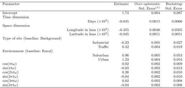
In order to estimate the frequency of this data set, we calculated the periodicity for each of the 88 monitoring sites. The median of these periodicities was equal to 365-day. So, in (4), we took ! to equal the inverse of the median and we obtained significative estimates for j,1 and j,2with j=1,2,3. The parameters estimates, and corresponding standard errors, are summarized in Table 2.
Table 2 Estimates of the parameters in model (4) for the daily averages of NO2concentrations, together with the
corresponding standard errors obtained by parametric bootstrap. The standard errors given in (⇤) were obtained by GLM when relaxing the assumption of non-correlated residuals.
Parameter Estimate Over-optimistic Bootstrap Std. Error(⇤) Std. Error Intercept 1.74 0.004 0.087 Time dimension Days (⇥103) -0.045 0.0015 0.0066 Space dimension Longitude in kms (⇥102) -0.455 0.0046 0.0505 Latitude in kms (⇥102) -0.045 0.0011 0.0051
Type of site (baseline: Background)
Industrial -0.23 0.005 0.027 Traffic 0.42 0.004 0.019 Environment (baseline: Rural)
Suburban 0.96 0.005 0.053 Urban 1.23 0.004 0.054 cos(⇡t!) 0.02 0.002 0.009 sin(⇡t!) -0.03 0.002 0.012 cos(2⇡t!) 0.26 0.002 0.010 sin(2⇡t!) -0.04 0.002 0.010 cos(3⇡t!) 0.02 0.002 0.008 sin(3⇡t!) -0.04 0.002 0.008
From the results in Table 2, the final fitted model shows a smooth decreasing behavior of the nitrogen dioxide levels over the years, as well as in latitude and longitude. In addition, we conclude that the values of NO2concentrations are greater in those monitoring stations where the environment is urban or suburban and the type of site is traffic, confirming the results from our exploratory analysis in Section 2. Indeed, the NO2concentrations increase by a factor of 3.4 from rural to urban and by a factor of 1.5 from background to traffic.
After estimation of the large-scale variation, given by the space-time trendµ(s, t), the resid-uals "(s, t) = Z(s, t) µ(s, t) can be computed, and the following step will be the structural
2 3 4 5 6 7 8 9 10 11 12 13 14 15 16 17 18 19 20 21 22 23 24 25 26 27 28 29 30 31 32 33 34 35 36 37 38 39 40 41 42 43 44 45 46 47 48 49 50 51 52 53 54 55
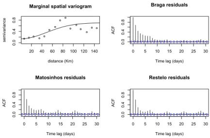
analysis of the resulting data to characterize the variability in the space and time components. As expected, after removing the trend, including the annual seasonality, our data still exhibits some temporal correlation, which in most of the cases is significative up to 8 to 12 days. For some particular monitoring stations, those close to urban areas, one may also find a weekly correlation, as weekends are typically associated to lower levels of NO2. Some examples are given in Fig. 3, where the marginal spatial semivariogram is displayed in the first pannel and the remainder ones show the autocorrelation functions in three monitoring stations.
20 40 60 80 100 120 140
0.0
0.4
0.8
Marginal spatial variogram
distance (Km) se mi va ria nce 0 5 10 15 20 25 30 0.0 0.4 0.8
Time lag (days)
AC F Braga residuals 0 5 10 15 20 25 30 0.0 0.4 0.8
Time lag (days)
AC F Matosinhos residuals 0 5 10 15 20 25 30 0.0 0.4 0.8
Time lag (days)
AC
F
Restelo residuals
Fig. 3 The upper left-hand side pannel displays the plots of the experimental spatial semivariogram (dots) and the fitted Gaussian model (solid lines). The remainder pannels show examples of autocorrelation functions (ACFs) for 3 monitoring stations (located in Braga, Matosinhos and Lisboa-Restelo)
.
The fit of the marginal variogram demands estimation of the unknown parameters of the theoretical model, namely, the nugget⌧2, the partial variance 2and the range (related to the distance beyond which there is no spatial or temporal correlation, also named radius of influence). The Gaussian model was selected for approximation of the spatial variogram, with time as a covariate, and the resulting parameter estimates were⌧2
s = 0.5, s2 = 0.38 and s = 55.88km. We have also considered other models, as the exponential one, obtaining similar estimates for the spatial covariance parameters.
With the aim of deciding whether to adopt the product-sum model (5) or the sum-metric model (6), to characterize the dependence structure of the residuals, we applied a cross-validation study to compare both models.
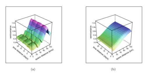
For computational reasons, the aforementioned approach was carried out by randomly choos-ing a subset of data from the whole set of 9 years, but always involvchoos-ing the total 88 monitorchoos-ing stations. Indeed, two random days were selected for each station, so that the corresponding obser-vations were eliminated from the original data set and then predicted from the remainder values. So, we proceeded as explained in Section 3, by eliminating each data from the whole set and then predicting it from the remainder values. With the resulting errors, for each of the selected mod-els combination, the mean error (ME) and the mean square error (MSE) were computed. Based on the observation of the empirical space-time variogram (Fig.4, left panel), together with the
2 3 4 5 6 7 8 9 10 11 12 13 14 15 16 17 18 19 20 21 22 23 24 25 26 27 28 29 30 31 32 33 34 35 36 37 38 39 40 41 42 43 44 45 46 47 48 49 50 51 52 53 54 55
observation of the marginal spatial variogram (Fig.3, top-left panel), our cross-validation study covers some specific combinations of the Gaussian and exponential models for each component in (5) and (6). The final results are presented in Table 3.
We conclude that similar results were achieved, which suggests to take into account the interpretation of each of the models as an additional argument for the final choice. In this respect, an important feature of the sum-metric model is to enable the use of specific variograms for space, time and space-time. Furthermore, it allows us to consider a spatio-temporal anisotropy parameter, that deals with the spatial and temporal distances in the same term. This led us to the selection of the sum-metric model for modeling the spatio-temporal dependence structure of NO2data.
Table 3 ME and MSE estimates of the cross-validation study, based on di↵erent spatio-temporal variogram families and di↵erent choices for the one-dimensional variogram components. This comparative study involved a subset of days randomly chosen from the complete set of 88 monitoring stations.
model joint temporal space ME MSE Product-sum model – Exp Gau -0.022 0.389 – Exp Exp -0.016 0.348 Sum-metric model Exp Exp Exp 0.018 0.433 Gau Exp Gau -0.019 0.369
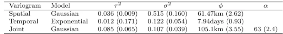
We then decided to choose a exponential function for the temporal variogram and Gaussian functions for the spatial and the spatio-temporal components. The resulting parameter estimates, which includes the anisotropy ratio ↵, are given in Table 4, where the corresponding standard errors were approximated by subsampling among the whole set of observed data. The fitted final model is represented in Fig. 4(b).
Table 4 Estimates of the parameters in the spatial, temporal and spatio-temporal variograms, together with the corresponding standard errors obtained by subsampling.
Variogram Model ⌧2 2 ↵
Spatial Gaussian 0.036 (0.009) 0.515 (0.160) 61.47km (2.62) Temporal Exponential 0.012 (0.171) 0.122 (0.054) 7.94days (0.93)
Joint Gaussian 0.085 (0.065) 0.107 (0.039) 105.1km (3.55) 63 (2.4)
According to the resulting space-time variogram, the majority of the total variation is ex-plained by the spatial and the spatio-temporal components, whereas the strictly temporal com-ponent has a much smaller contribution. The values achieved also suggest that NO2 underlies a significative spatial correlation up to 60 kms and a temporal correlation up to 8 days. In addition, this information highlights the importance of considering a joint component, as the corresponding estimates seem to give evidence of a significative time-space interaction. Further-more, a complete separation of the spatial and temporal components would imply that spatial patterns are identical at all time points and that temporal dynamics are the same everywhere, which we believe that it would not apply for the data collected.
Following the estimation of the small-scale variation, specified by the space-time variogram, one may proceed with a parametric bootstrap approach to obtain accuracy measures of all the parameters estimates involved in the 2-stepwise modelling procedure described in Section 3. In
2 3 4 5 6 7 8 9 10 11 12 13 14 15 16 17 18 19 20 21 22 23 24 25 26 27 28 29 30 31 32 33 34 35 36 37 38 39 40 41 42 43 44 45 46 47 48 49 50 51 52 53 54 55
0 20 4060 80100 0 5 10 15 20 0.0 0.2 0.4 0.6 0.8 1.0 space distance (kms) time dist ance (d ays) se mi va ria nce (a) 0 20 4060 80100 0 5 10 15 20 0.0 0.2 0.4 0.6 0.8 1.0 space distance (km) time dist ance (d ays) se mi va ria nce (b)
Fig. 4 Plots of the experimental estimator (a) and the fitted model (b) for the space-time semivariogram.
particular, the standard errors for the regression coefficients of the trend, presented in the last column of Table 2, were derived as the standard deviation of point estimates of 500 bootstrap replicates, drawn from a multivariate normal distribution, with expectation exp(⌘(s, t)), as given in (4), and a covariance matrix obtained from the sum-metric model st(hs, ht) in (6).
4.2 Space-time kriging
Having in mind that, for this Portuguese case study, about 30% of the daily observations over the 9 years of observation are missing, prediction is a very important further step in this work. This high percentage is a consequence of many factors, such as the regular calibration and maintenance of the monitoring stations. Moreover, one must take into account that, during the study period, the monitoring network have been su↵ering some modifications, namely some stations were being closed and new ones were being added to the network. In fact, at the end of the study, end of 2012, there were 21 monitoring stations classified as “inactive”. Additionally, it is important to be able to predict NO2 concentrations at unobserved spatial points. The use of the space-time kriging techniques, to be applied at any space-time point, proves a very convenient approach to mitigate these problems.
Table 5 Main characteristics of Braga, Matosinhos and Restelo (Lisboa) monitoring stations. Type of site Type of environment Status Missing days in 2012 Braga background suburban active 6
Matosinhos traffic urban inactive 366 Restelo background urban active 13
To illustrate these ideas, we selected the 3 specific monitoring stations, whose characteristics are summarized in Table 5, one located in Braga (north of Portugal) and the other two in Restelo and Matosinhos, as they cover Lisbon and Porto areas, respectively. The three aforementioned zones correspond to densely populated areas of great industrial activity.
A summary of the results is presented in Figures 5 and 6, representing the estimation of the large-scale and small-scale variations of NO2, respectively. The former figure shows a 95%
2 3 4 5 6 7 8 9 10 11 12 13 14 15 16 17 18 19 20 21 22 23 24 25 26 27 28 29 30 31 32 33 34 35 36 37 38 39 40 41 42 43 44 45 46 47 48 49 50 51 52 53 54 55
Braga 2012 Time (days) NO2 0 100 200 300 0 20 40 60 Matosinhos 2012 Time (days) NO2 0 100 200 300 0 20 40 60 Restelo 2012 Time (days) NO2 0 100 200 300 0 20 40 60
Fig. 5 Estimation of the large-scale variation of NO2concentrations over 2012 for 3 monitoring stations: Braga,
Matosinhos and Restelo (Lisboa). In the case of Matosinhos, there are no observed data available, otherwise this is represented by a black full-line. For Braga and Restelo, one has 6 and 13 missing values over 2012, respectively. The red dashed-lines identify the 95% confidence band for the estimated trend, obtained by parametric bootstrap. The grey horizontal dashed-line represents the annual mean limit of 40µg/m3
dence band for the estimated trend at each monitoring station, which is obtained by parametric bootstrap, as described in Section 4.1. In particular, as Matosinhos station became inactive in 2012, this procedure allows us to derive the expected NO2values along that year and, therefore, to conclude that the concentrations of NO2may range from 28.1µg/m3to 49.8µg/m3, with an estimated median value of 35.9µg/m3. Figure 6 takes into account the small-scale variation, rep-resented by the kriging predictions over 2012 of the residuals in (1) for the 3 monitoring stations. One should note that the variability patterns of the predicted residuals time series and the NO2 time series in Figure 5 (for Braga and Restelo cases) are as expected very similar.
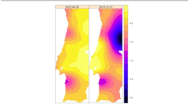
To conclude, Figure 7 presents the predicted maps for two time points chosen as representative of the summer peak (2012-06-30) and the winter peak (2012-12-31). The results confirm that the general spatial pattern of the NO2 concentrations is not persistent over time, being the spatial variability significatively higher in winter than in summer. In fact, the predicted values for that day of December allow to clearly identify an area with high values near Lisbon and north of Lisbon, and that is not occurring in June. Finally, for the interpretation of results, one should have in mind that most monitoring stations are in cost areas of Portugal, so associated to smaller prediction errors. 2 3 4 5 6 7 8 9 10 11 12 13 14 15 16 17 18 19 20 21 22 23 24 25 26 27 28 29 30 31 32 33 34 35 36 37 38 39 40 41 42 43 44 45 46 47 48 49 50 51 52 53 54 55
Prediction 2012 - Braga Time (days) re si du al s N O 2 0 100 200 300 -1 .5 -0 .5 0.5 1.5 Prediction 2012 - Matosinhos Time (days) re si du al s N O 2 0 100 200 300 -1 .5 -0 .5 0.5 1.5 Prediction 2012 - Restelo Time (days) re si du al s N O 2 0 100 200 300 -1 .5 -0 .5 0.5 1.5
Fig. 6 Estimation of the small-scale variation, obtained from the kriging predictions over 2012 of the residuals in (1) for 3 monitoring stations: Braga, Matosinhos and Restelo (Lisboa). Black lines are predictions along with corresponding 95% prediction intervals (grey lines) and, when available, the blue dots identify the observed residuals.
5 Conclusions
There is an increasing concern about the air pollution, because of the important problems derived from it. That is the reason why many countries have developed an extra e↵ort to set up a system of monitoring stations, so as to collect a qualified database of di↵erent elements involved in the estimation of the ambient air quality. From the information achieved, we focussed our attention on the spatio-temporal evolution of the NO2concentration data, due to the significant environmental and health risks associated to this pollutant, by considering the data set collected in Portugal in the period 2004-2012. The current research also studies the e↵ect of di↵erent factors on the levels of NO2detected, such as the type of site where the station is placed (background, industrial and traffic), the environment of the zone (urban, suburban and rural) or the month when the target variable is measured.
A first analysis showed the influence of the above-mentioned covariates on the NO2levels. In fact, the higher values were observed on the urban or suburban zones, as well as on the traffic areas, whereas the industrial type of site seems to be a factor with preventive e↵ect. In addition, the exploratory study also gave account of the asymmetric distribution of the NO2 data and their decreasing trend in the period 2004-2012.
Next, we addressed the estimation of the trend function by using a mixed model, involving the generalized linear model, with the type of site and environment as explanatory variables, as
2 3 4 5 6 7 8 9 10 11 12 13 14 15 16 17 18 19 20 21 22 23 24 25 26 27 28 29 30 31 32 33 34 35 36 37 38 39 40 41 42 43 44 45 46 47 48 49 50 51 52 53 54 55
Fig. 7 Space kriging maps at two arbitrary days: 2012-06-30 (left) and 2012-12-31 (right).
well as other functions to incorporate seasonality and long-term trend components. According to the acquired coefficient of determination, about 43% of the large-scale variation of the NO2 concentrations is explained under this trend model. The following step was to adequately charac-terize the underlying space-time dependence, where the final variograms were obtained by fitting the empirical estimators to the valid models that were selected by taking into account the role played by the components involved in each of them.
For a comparison of the di↵erent proposals, we applied a cross-validation approach showing that an adequate option was provided by the characterization of the space-time variability of the residuals through a sum-metric fit, with a major contribution of the purely spatial and the spatio-temporal components.
Knowledge of the space-time dependence could have been the aim of this study, as this information would help optimize the monitoring design itself or complement the current one, where there are districts without monitoring stations. It also enables us to apply the interpolation techniques for characterization of the spatio-temporal patterns of the NO2data, without requiring data from a dense monitoring network. So, we can assess the nitrogen dioxide concentrations at sites where either data have been lost or there is no monitoring station nearby. These potentialities of our research have been illustrated for some specific cases and it could be extended over time and space.
References
Bivand R, Pebesma E, G´omez-Rubio V (2008) Applied Spatial Data Analysis with R. Springer, New York
Bogaert P (1996) Comparison of kriging techniques in a space-time context. Mathematical Ge-ology 28:73–86
Bruno F, Guttorp P, Sampson P, Cocchi D (2009) A simple non-separable, non-stationary spa-tiotemporal model for ozone. Environmental and Ecological Statistics 16:515–529
2 3 4 5 6 7 8 9 10 11 12 13 14 15 16 17 18 19 20 21 22 23 24 25 26 27 28 29 30 31 32 33 34 35 36 37 38 39 40 41 42 43 44 45 46 47 48 49 50 51 52 53 54 55
Calculli C, Fasso A, Finazzi F, Pollice A, Turnone A (2015) Maximum likelihood estimation of the multivariate hidden dynamic geostatistical model with application to air quality in apulia, italy. Environmetrics 26:406–417
Cameletti M, Ignaccolo R, Bande S (2011) Comparing spatio-temporal models for particulate matter in piemonte. Environmetrics 22:985–996
Carslaw DC (2005) Evidence of an increasing no2/nox emissions ratio from road traffic emissions. Atmospheric Environment 39:4793–4802
Cressie N (1990) The origins of kriging. Mathematical Geology 22:239–252
Cressie N, Huang H (1999) Classes of nonseparable, spatio-temporal stationary covariance func-tions. Journal of the American Statistical Association 94:1330–1340
Cressie N, Wikle C (2011) Statistics for spatio-temporal data. John Wiley and Sons, New York De Cesare L, Myers D, Posa D (2001) Estimating and modeling space-time correlation structures.
Statistics and Probability Letters 51:9–14
De Gruijter J, Brus D, Bierkens M, Knotters M (2006) Sampling for Natural Resource Monitor-ing. Springer, Germany
De Iaco S, Posa D (2012) Predicting spatio-temporal random fields: Some computational aspects. Computers & Geosciences 41:12–24
Dimitrakopoulos R, Luo X (1994) Spatiotemporal modeling: covariances and ordinary kriging systems. In: Dimitrakopoulos, R. (ed.), Geostatistics for the next century, Kluwer Academic Publishers, Dordrecht, pp 88–93
Dimitrakopoulos R, Luo X (1997) Spatiotemporal modeling: covariances and ordinary kriging systems. In: Baafi, E. and Scofield, N. (eds.), Geostatistics Wollongong’96, Kluwer Academic Publishers, Dordrecht, pp 138–149
Fern´andez-Casal R, Gonz´alez-Manteiga W, Febrero-Bande M (2003) Flexible spatio-temporal stationary variogram models. Statistics and Computing 13:127–136
Fox J (2008) Applied Regression Analysis and Generalized Linear Models. SAGE Publications Gneiting T, Genton MG, Guttorp P (2007) Statistical Methods for Spatio-Temporal Systems.
Chapman and Hall, Cambridge
Goovaerts P (1997) Geostatistics for natural resources evaluation. Oxford University Press, New York
Grice S, Stedman J, Kent A, Hobson M, Norris J, Abbott J, Cooke S (2009) Recent trends and projections of primary no2 emissions in europe. Atmospheric Environment 43:2154–2167 Heuvelink G, Griffith D (2010) Space-time geostatistics for geography: A case study of radiation
monitoring across parts of germany. Geographical Analysis 42:161–179
Host G, Omre H, Switzer P (1995) Spatial interpolation errors for monitoring data. Journal of the American Statistical Association 90:853–861
Isaaks E, Srivastava R (1989) An Introduction to Applied Geostatistics. Oxford University Press, New York
Kyriakidis P, Journel A (1999) Geostatistical space-time models: A review. Mathematical Geol-ogy 31:651–684
Lewne M, Cyrys J, Meliefste K, Hoek G, Brauer M, Fischer P, Gehring U, Heinrich J, Brunekreef B, Bellander T (2004) Spatial variation in nitrogen dioxide in three european areas. Science of the Total Environment 332:217–230
Lindley S, Walsh T (2005) Inter-comparison of interpolated background nitrogen dioxide con-centrations across greater manchester, uk. Atmospheric Environment 39:2709–2724
Myers D (2004) Estimating and Modeling Space-Time Variograms. In: McRoberts, R. (ed.), Proceedings of the joint meeting of TIES-2004 and ACCURACY-2004
Porcu E, Mateu J, Saura F (2008) New classes of covariance and spectral density functions for spatio-temporal modelling. Stochastic Environmental Research and Risk Assessment 22:65–79 2 3 4 5 6 7 8 9 10 11 12 13 14 15 16 17 18 19 20 21 22 23 24 25 26 27 28 29 30 31 32 33 34 35 36 37 38 39 40 41 42 43 44 45 46 47 48 49 50 51 52 53 54 55
R Team D (2010) R: A Language and Environment for Statistical Computing. R Foundation for Statistical Computing
Rodriguez-Iturbe I, Mej´ıa J (1974) The design of rainfall networks in time and space. Water Resources Research 10:713–728
Rouhani S, Hall T (1989) Space-Time Kriging of groundwater data. In: Armstrong, M. (ed.), Geostatistics, Kluwer Academic Publishers, Dordrecht, pp 639–651
Saiz-Lopez A, Adame J, Notario A, Poblete J, Bol´ıvar J, Albaladejo J (2009) Year-round obser-vations of no, no2, o3, so2 and toluene. Water, Air and Soil Pollution 200:277–288
Shaddick G, Yan H, Salway R, Vienneau D, Kounali D, Briggs D (2013) Large-scale bayesian spatial modelling of air pollution for policy support. Journal of Applied Statistics 40:777–794 Stedman J, Goodwin J, King K, Murrells T, Bush T (2001) An empirical model for predicting urban roadside nitrogen dioxide concentrations in uk. Atmospheric Environment 35:1451–1463 Stein M (2005) Space-time covariance functions. Journal of the American Statistical Association
469:310–320
Stone M (1974) Cross-validatory choice and assessment of statistical predictions. Journal of the Royal Statistical Society B 36:111–133
WHO (2003) Health Aspects of Air Pollution with Particulate Matter, Ozone and Nitrogen Dioxide. World Health Organization, Germany
2 3 4 5 6 7 8 9 10 11 12 13 14 15 16 17 18 19 20 21 22 23 24 25 26 27 28 29 30 31 32 33 34 35 36 37 38 39 40 41 42 43 44 45 46 47 48 49 50 51 52 53 54 55