Construction and Visualization of Concept Prerequisite Graphs for E-Learning
by
Mehmet Cem Aytekin
Submitted to the Graduate School of Engineering and Natural Sciences in partial fulfilment of
the requirements for the degree of Master of Science
Sabancı University July 2019
© Mehmet Cem Aytekin 2019 All Rights Reserved
Acknowledgements
This thesis would not be possible without the support of some important people in my life. It also cannot be finalized without expressing my gratitude to them.
Firstly, I would like to express my sincere gratitude to my thesis advisor, Prof. Dr. Y¨ucel Saygın for his support throughout my graduate studies. His clever, practical and effective solutions to the seemingly complex and hard problems gave me confidence not only in my research but also in my other studies at the university. Without his guidance and careful supervision this thesis would not be where it is now. I also owe a debt of gratitude to all instructors in CS department for imparting their knowledge to me.
Last, but not the least, I would also like to thank to my parents who have been around at every step of my life to motivate me. They lived all ups and downs of my academic journey and shared my excitement with me.
CONSTRUCTION AND VISUALIZATION OF CONCEPT PREREQUISITE GRAPHS FOR E-LEARNING
Mehmet Cem Aytekin
Computer Science and Engineering, Master’s Thesis, 2019 Thesis Supervisor: Y¨ucel SAYGIN
Keywords: e-learning, concept maps, prerequisite relations, prerequisite graphs for online learning, wikipedia articles, machine learning in online education.
Abstract
The growth of internet technologies in the last decade allowed the knowledge to spread out very fast across the globe. Users began educating themselves with huge amounts of online material on the internet. Today many academic institutions offer publicly available courses where students all around the world can join and benefit from them.
The abundance of online material from many different resources created an unor-ganized content in which it is likely for the learners to get lost. Furthermore, some concepts may require knowledge from other concepts and the learner may not be aware of those prerequisite relations between the concepts, therefore, she may have difficulties in understanding them.
In our work, we propose a methodology for calculating prerequisite scores among text-based educational material. We choose Wikipedia articles to work with since it is a large encyclopedia containing huge amounts of information on lots of differ-ent concepts. Furthermore, from a given set of concepts with their corresponding Wikipedia articles, we calculate each concept’s prerequisite score towards other con-cepts and build a prerequisite concept graph for the learner. We believe that our graph model will guide the students in their studies and enhance their learning experience.
C¸ EVR˙IM˙IC¸ ˙I E ˘G˙IT˙IM ˙IC¸ ˙IN KAVRAM ¨ONKOS¸UL HAR˙ITALARININ OLUS¸TURULMASI VE G ¨ORSELLES¸T˙IR˙ILMES˙I
Mehmet Cem Aytekin
Bilgisayar Bilimi ve M¨uhendisli˘gi, Y¨uksek Lisans Tezi, 2019 Tez danı¸smanı: Y¨ucel SAYGIN
Anahtar Kelimeler: online e˘gitim, kavram haritasi, ¨onko¸sul ili¸skisi ,¨onko¸sul haritalari ,Wikipedia makaleleri, online e˘gitimde makine ¨o˘grenmesi
¨
Ozet
Son on yılda internet teknolojilerinin hızlı geli¸simi bilginin d¨unyanın her yerine ¸cok kolay bir ¸sekilde yayılmasına izin vermi¸stir. ˙Internet ortamındaki bilgi bollu˘gu sayesinde kullanıcılar kendilerini geli¸stirmeye fırsat bulmu¸stur. G¨un¨um¨uzde bir ¸cok akademik kurum herkesin kullanımına a¸cık dersler sunmaya ba¸slamı¸s ve d¨unyanın bir ¸cok yerinden ¨o˘grenciler bunlara katılıp yararlanma imkanı elde etmi¸stir.
Neredeyse her konuyla ilgili bir ¸cok farklı kaynaktan yapılan payla¸sımlar her ne kadar ¨o˘grenciler i¸cin bir avantaj gibi g¨oz¨ukse de t¨um bu bilgi yı˘gını, ¨o˘grenilmek iste-nilen konunun internette d¨uzensiz ve karma¸sık bir ¸sekilde sunulmasına yol a¸cmı¸stır. Bu y¨uzden ¨o˘grencinin ilgili oldu˘gu konuyu ¨o˘grenmeye ¸calı¸sırken t¨um bu karma¸sa i¸cinde kaybolması olasıdır. Daha da ¨onemlisi, ¨o˘grenilmek istenen konu bir ¸cok teknik kavram gerektirebilir ve bu kavramlardan bazıları, di˘ger kavramları anlamak i¸cin ¨on ko¸sul olabilir. Bu durumda ¨o˘grenci konuyu ¨o˘grenmeye hangi kavramlardan ba¸slamalı bilemeyebilir ve dolayısıyla b¨ut¨un konuyu kavramakta zorluk ya¸sar. Bu temel problemden yola ¸cıkarak ¸calı¸smamızda, ¨oncelikli olarak iki farklı kavramı anlatan yazılı akademik d¨ok¨umanın arasında olabilmesi muhtemel ¨onko¸sul ili¸skisini sayısal olarak ifade etmeye ¸calı¸sıyoruz. Kavramlarla ilgili yazılı d¨ok¨umanları hemen hemen her konudan bilgi i¸ceren ve ¸cok b¨uy¨uk bir ¸cevrimci ansiklopedi olan Wikipedia’dan makale olarak alıyoruz. Bununla beraber, konuyla ilgili ¨o˘grenilmek istenilen
kavram-lar, Wikipedia makale kar¸sılıkları ile verilirse t¨um bu kavramların birbiri ile olan ¨
onko¸sul ili¸skilerini hesaplayıp bunlardan bir ¨onko¸sul kavram haritası olu¸sturarak ¨
o˘grenciye sunuyoruz. Olu¸sturdu˘gumuz haritanın yeni bir konuyu ¸cevrimci ¨o˘grenmek isteyen bir kimseye ¨o˘grenme s¨urecinde faydalı olmasını umuyoruz.
Table of Contents
Acknowledgements iv Abstract v ¨ Ozet vi 1 Introduction 11.1 Overview of the Methodology and Contributions . . . 3
2 Related Work 6 3 Methodology and Problem Definition 11 3.1 Prerequisite Score Calculation . . . 12
3.1.1 Definition of the Score Function . . . 12
3.1.2 Input Format and Feature Selection . . . 12
3.1.3 Weight Learning . . . 14
3.1.4 Testing the Scoring Function . . . 15
3.2 Graph Formation . . . 17
3.2.1 Prerequisite Matrix . . . 17
3.2.2 Matrix Filtering and Graph Building . . . 17
3.3 Different Levels of Generalizations in the Graph . . . 21
4 Implementation, Experiments, and Evaluation 24 4.1 Prerequisite Score Accuracy . . . 24
4.2 Graph Formation . . . 27
4.2.1 Complexity of the Algorithm . . . 27
4.2.2 Physics data-sets . . . 28
4.2.3 Database Management System Concepts . . . 31
4.3 Graph Generalization . . . 32
5 Conclusion and Future Work 37
A Tabular results of evaluations on each data-set 39
List of Figures
3.1 Weight Learning of our Score Function . . . 16
3.2 Forming the Graph Model . . . 19
4.1 General View of the Graph . . . 28
4.2 View of Cluster 1 and Cluster 2 . . . 29
4.3 View of Cluster 3 and Cluster 4 . . . 30
4.4 General View of the Graph . . . 31
4.5 Second Level Physics Graph . . . 34
List of Tables
4.1 Prerequisite Scores . . . 32 A.1 Evaluations on physics data-set with a threshold value of 0.8. . . 39 A.2 Evaluations on physics data-set with a threshold value of 0.8. . . 40 A.3 Evaluations on database management systems data-set with a
Chapter 1
Introduction
Online learning has grown exponentially during the first decade of the twenty-first century due to the rapid advancements in internet technologies. Many large colleges and universities began putting their course materials on the internet and making it publicly available to everyone who is interested in learning a particular subject. There are also a number of growing online encyclopedias, especially Wikipedia which is the largest and most popular general reference work on the World Wide Web with more than 300.000 active users and thousands of contributors from all around the world [1].
The abundance of online technical material on the internet accelerated the process of reaching out to specific information. However, this simplicity has also brought certain disadvantages along with it.
The major challenge for the learner is to be able to choose the right resources among a huge amount of online materials. The particular concept she is trying to learn may require some background knowledge, in that case, the learner should be able to identify the other concepts that are necessary to understand that particular concept and start studying them first.
Another challenge is the lack of a generalization mechanism in the huge concept pool. The concepts may belong to very specific areas and may contain very detailed information which in return prevents the learner from being able to look at those concepts at a broader level. It is always helpful for the learner when the discussed content is presented in an organized way. For instance, in a book, we have chapters,
sections, and sub-sections so whenever we refer to a specific concept in a book, we have an idea of where we are in the global context.
The last difficulty is the variety in the learning process itself. Even if two different learners have the same level of background, their learning styles may be different. Some people may learn better with visual material whereas some may learn better with text-based material. Hence the learner also needs to be able to recognize her learning style and choose the right kind of online resource accordingly.
What should one know first before trying to learn a new concept? The answer to that question relies on the notion prerequisite. As defined in the Cambridge dictionary [2], a prerequisite is something that must exist or happen before something else can exist or happen. In this thesis, a prerequisite defines a relationship among two concepts A and B. We define it as a score between [-1 and 1] where the sign indicates the direction of this relationship and the score gives us the strength of the prerequisite.
Our work aims to build a complete weighted graph structure out of all the pre-requisite scores between concept pairs. More technically, given a set of concepts
C ={C1, C2, ..., Ck} we want to build a score matrix S
S = s11 · · · s1k .. . ... ... sk1 · · · skk
where sij is the prerequisite score between the ith and jth concept.
Using the concept listC and the score matrixS, we construct our graph where nodes in the graph represent the concepts in the list C and the elements of the matrix S
represent the directed weighted edges among nodes.
The constructed graph is then presented to the learner where she sees all the concepts and their degree of prerequisite relations with each other by looking at the nodes and the directed edges of the graph. If the learner wants to master a specific target topic ct but she is not sure whether that topic ct requires some knowledge from the
for the target topic by following the incoming edges to ct in the graph and master
them first in order to completely understand the concept ct. If these concepts are
also not familiar to her, then the learner can go back once more and repeat the above procedure recursively until arriving at the concepts in the graph that she feels hundred percent confident about. Beginning from those known concepts, the learner can this time go forward and start studying the prerequisite concepts along the way until she reaches the target concept ct. Finally, with enough knowledge
gained along the way, the learner can master the concept ct and move on.
Furthermore, when we analyze the constructed graph, we observe natural clusters within the structure. It is expected to have this sort of disconnected components in the graph since any unrelated concept pair will likely to have zero prerequisite score in between. It is also possible to conclude that the concepts in the naturally formed clusters are related to each other to some degree, therefore, we have a grouping. These clusters can be thought of as first level generalizations of the concepts in the given concept set. Treating each cluster as a one level generalized concept, their inter-prerequisite scores can again be calculated which yields second level generalized clusters. This procedure can go on until we are left with one cluster which represents the highest level of generalization.
1.1
Overview of the Methodology and
Contribu-tions
Calculating a score for a prerequisite relationship between two concepts is not a straightforward task. In general, an online educational material revolves around the main concept and is presented to the user in various forms such as text, audio, image or a video. In this thesis, a concept is represented by a Wikipedia article, which may be considered as a text-based online educational material. When we refer to concepts A and B, we need to fetch the corresponding articles A and B from Wikipedia. Since Wikipedia is a vast encyclopedia, it is often possible to find the corresponding articles easily. Furthermore, Wikipedia offers its Wikipedia library to developers which makes it easy to query any article and get detailed information
about it.
Our initial work starts by exploring which properties of the two Wikipedia articlesA
andB can give us information about the prerequisite relationship between them and we determine several important features that we will explain in detail in Chapter 3.1. Moreover, after discovering the relevant features, we apply a standard supervised machine learning technique to determine the weights of these discovered features. The data-set that is used in the weight learning process is the famous university course data-set first introduced by Liang et al. 2017 in [3] where 1008 Computer Science topics are listed and labeled according to their prerequisite relation by the domain experts.
After having learned the features and their corresponding weights, our model be-comes ready to assess the prerequisite relation of a concept pairAand B, and gives a score to them between -1 and 1 where -1 means A is a complete prerequisite ofB
and 1 means B is a complete prerequisite ofA and anything in between shows the degree of their relationship.
Although the score prediction part of the system makes our approach a regression type of solution, it is also possible to use the system as a classifier such that if the score of a pair A and B is above 0, then conceptB is a prerequisite of A, if 0, then there is no prerequisite relation and if below 0, then A is a prerequisite ofB. To test the performance of our system, we make use of the classification property of our system and ask it to classify the different concept pair instances from different labeled data sets and report the classification accuracies. We also choose prerequisite pairs from different domains and show that although our method is trained with computer science topics, it performs still well in other fields as well.
Finally, on the same data-set, we perform two other prerequisite calculation meth-ods which are similar to ours and make comparisons of our approach with those approaches.
In Chapter 3, we look at the idea of the concept maps which attempt to capture the concepts and their relationships among them in a given educational material. Elaborating on this idea, we specialize our focus on a specific type of relationship,
namely the prerequisite relationship and discuss the ways to identify it by giving references to the existing literature. In Chapter 3, we explain how we calculate the prerequisite relationships and build a graph from the given concepts in detail. We also discuss the ways to generalize the given concepts and rebuilding graphs in different hierarchical levels. In Chapter 4 we analyze the performance of our system on different data-sets from different domains and report the results in detail. We also try to understand the weak and strong sides of our algorithm. In Chapter 5 we describe the limits of our algorithm and we suggest possible ways to overcome them. We explain how the students can benefit from our system and how it can be further developed for online learning.
Chapter 2
Related Work
The search for a visual representation of knowledge has long been an occupation for the researchers in computer science. One of the successfully adapted and widely used technique for this task is concept mapping [4]. It attempts to capture the subjects in the context as concepts, draws them with a special symbol, tries to name their inter-relationships and links them one to another with arrows. Concept maps are especially useful in the field of education and facilitate the learning process of the students.
The idea of a concept map comes with its challenges and part of those challenges have been an inspiration for our work. The main challenge is the need for an expert when building a concept map. In theory, the expert should be able to list all the relevant concepts and be able to define their relationships with each other in a given context. However, the context may be complex and the relation between the concepts may not be obvious. Moreover, each context requires a different concept map and no expert in the world has enough knowledge to combine those maps together to build a universal concept map. This major problem then raises the question: Can it be possible to automate the process of concept map creation?
The first challenge in the automation process is the extraction of subjects or namely concepts in the given context. The second challenge is to define the relationship between the two concepts. Considering the relationship as an interaction between two subjects, there may be huge amounts of possible relations between a concept pair (A, B) such that concept A can be a part of concept B, or it can be a prerequisite
of B or it can simply be the detailed version ofB, etc. These two major difficulties have been the focus points of the researchers who wanted to build automatic or semi-automatic concept maps.
In the search for a semi automatic concept map creation, one tool that grabbed the attention in the area is TextStorm and its extension Clouds [5], [6]. When the context is given as a text document, TextStorm identifies the subject, object, and verb by parsing each sentence in the document. The subject becomes the first con-cept; the object becomes the second concept, and the verb defines their relationship. From there on, TextStorm takes the candidate concepts and relationships and feeds them into Clouds. After getting input from TextStorm, Clouds asks questions to domain expert about the concept-verb-concept structures it formed and it attempts to generalize its knowledge by using inductive logic and outputs a concept map in the end. One good example to understand the generalization process is given in the paper as follows [7]: If it is observed that: produce (apple tree; apple)produce (pear tree; pear) and from the domain knowledge, it is known that isa (pear tree; tree)
isa (apple tree; tree) isa (pear; fruit) isa (apple; fruit) a generalization is deduced
produce (tree; fruit).
Other approaches to capture relevant concepts are based on converting the text documents into vector representations by using standard approaches such as Bag of Words and TFIDF weighting [8], [9]. After turning documents into vectors, the term-document matrix is constructed where the rows correspond to terms and columns correspond to documents. Then by applying Latent semantic analysis technique, it is possible to cluster the documents that share similar words [10]. One can then look at the most referenced word in each document cluster and come up with a list of words representing the main concepts in all the documents. If the context is considered as a set of documents then the above approach is one way of doing concept extraction in a large textual resource. However, these series of techniques do not solve the problem of defining the relationships among the concepts. They only attempt to provide a solution for the first challenge mentioned at the beginning of this chapter.
dictionaries to deal with concept extraction problem. Given a specific context, the expert can predetermine the necessary concepts and build a dictionary out of them so that whenever the system receives a text resource about that particular con-text, it can quickly identify the relevant concepts in it by looking at the dictionary. Having concepts in advance, several association measures from information theory and statistics such as pointwise mutual information [12] are proposed in the litera-ture to quantify the relatedness of the relevant concepts appearing in the same text resource.
Om P. Damani took Pointwise Mutual Information (PMI) technique as a base and then developed the significant co-occurence idea to discover the meaningful associ-ations among concepts both at document and corpus level [13] [14]. The main idea in PMI is that to have a meaningful association score, the probability of observing concepts A and B together should be high and the probability of observing them individually should be low in a given text. A new probability function is defined for calculating the joint probabilities of conceptA andB appearing in close ranges and the results of these probabilities are used to determine whether their co-occurence shows any statistical significance or not.
It is important to state that although co-occurence indicates a relatedness between two concepts, it does not imply causality and still it does not define what type of relationship exists between two concepts.
In this thesis, we concentrate on a specific type of relationship, namely the pre-requisite relationship between two concepts. Moreover, we also assumed that the concepts are pre-defined by the expert.
Tseng et al. proposed an interesting way of automatic concept map creation in 2005 by considering the prerequisite relationships among concepts [15]. They proposed a Two-Phase Concept Map Construction (TP-CMC) algorithm to automatically construct a concept map of a course by historical testing records. The test record contents were known in advance and the authors assumed that concepts asked in some test A are prerequisites of some other concepts in test B, if lots of students have either high or low scores in both tests. By matching a group of concepts as the prerequisites of other concepts, they formed a concept map where the nodes are the
individual concepts and the weighted directed edges are the prerequisite strengths together with the prerequisite directions. A similar approach is used by Yang et al. where they analyzed course prerequisites from different university databases to learn a directed universal concept graph, and they used the induced graph to predict unobserved prerequisite relations among a broader range of courses [16].
The other idea for determining a prerequisite relationship is to treat each concept as a possible Wikipedia article and calculate prerequisite scores for the articles. To the best of our knowledge, this idea was first mentioned by Talukdar and W. Cohen [17]. They mention the nice properties of Wikipedia in textual analysis such as the densely linked structure of the site, its standardized format, and information available about how documents are used by the Wikipedia community.
The idea of using Wikipedia articles for determining prerequisite relation between concepts is further analyzed by Liang et al.[18]. They defined a metric called ref-erence distance (RefD) which takes two Wikipedia articles as inputs and outputs a prerequisite score between 1 and -1 where the sign indicates the direction of the prerequisite and the score demonstrates the strength of the prerequisite.
The articles in Wikipedia have hyperlinks. The domain specific terms that are important in understanding the article are underlined with blue color by the editors. Whenever the reader is unfamiliar with the underlined term, she can move to the article that explains it by clicking on it.
These hyperlinks that are in some article A, are considered as related to A. Chen Liang et al. called these hyperlinks inside A, as the concept space of A [18]. The observation is that given two articles A and B, if most of the concepts in concept space ofArefer to articleB, this may indicateB is a prerequisite ofAsince in order to understand the related concepts of A we have to know concept B in advance. The vica versa is also valid.
The reference distance calculation is based on this above observation. Given two articles A and B, the ratio of concepts referring to B to the number of concepts in concept space A yields a score between 0 and 1. This score can be interpreted as how much B is a prerequisite of A. Applying the same logic, the ratio of concepts
referring to A to the number of concepts in concept space B again yields a score between 0 and 1. This second score can be interpreted as how much A is a pre-requisite of B. Finally, the difference between these two scores gives us a number between -1 and 1 which constitutes the reference distance score.
Elaborating on this method, we discovered that it is possible to add more fea-tures to RefD formula due to the abundant information available for the articles in Wikipedia.
We observed that only considering the concept spaces of articles A and B are not enough and we should also consider the references in the articles themselves. More-over, it is also important how many timesAitself referenced B or vica versa. These considerations are not taken into account in plain RefD calculation.
It is also possible to read the summary of the articles in Wikipedia. We concluded that if the conceptArefers to the concept B in its summary, then this concept ofB
must be valuable forA since the summaries are short and only the most important aspects of the concepts are presented to the user. Therefore we also included the summary reference count into the refD formula.
Furthermore, we know that not every feature about an article is at the same impor-tance when calculating a prerequisite score, so with the help of the existing labeled prerequisite data-sets, we approximated the weights of those features by applying machine learning techniques. Details of these techniques and the stages of the whole procedure are discussed in Chapter 3.
Chapter 3
Methodology and Problem
Definition
In this chapter, we explain and discuss in detail how we construct the prerequisite graph from a given set of concepts. Our algorithm has three main stages:
• Stage 1: Prerequisite score calculation between two concepts,
• Stage 2: Building a graph out of the prerequisite scores calculated in the first stage
• Stage 3: Clustering and generalizing the given concepts by using the hierar-chical property of our graph.
The process in the first stage has four major steps. We first start by defining our score function and objective then we move to the data preparation part and explain which type of data we use and how we determine the relevant features. After that, we reach to learning part where we determine the weights of the features by supervised learning. We finally interpret our results on the test data and finish the first stage in our algorithm. The second stage has two major steps. At the first step we calculate each concept’s prerequisite score with the other concepts in the list and we build a prerequisite score matrix. At the second step we make simplifications on the score matrix and then turn it into a graph model. Finally, in the third stage, we show different levels of concept generalizations on the graph.
3.1
Prerequisite Score Calculation
In order to give a score for given concepts, we should define a mathematical function
f and describe all its properties in detail.
3.1.1
Definition of the Score Function
The arguments: Our function takes two concept names as inputs. In order for these arguments to be valid, these two concepts should have their corresponding articles in Wikipedia with the same name.
The output: Function outputs a score between -1 and 1.
Asymmetry: Given concept names A and B, f(A, B) +f(B, A) = 0. Irreflexivity:f(A, A) = 0.
3.1.2
Input Format and Feature Selection
Having found the corresponding Wikipedia articles for the conceptsA and B, three features are analyzed by our function. The first feature is RefD score for the articles
A and B. (Detail about RefD score is in Related Work). This score computes how much of the neighbour concepts ofArefer to conceptB. If most of the neighbours of conceptArefer toB, this indicates a possible prerequisite relationship fromB toA. The second feature is the number of reference different count in the articles A and
B themselves. For example, if the conceptAitself refers toB 15 times in its article and concept B refers to concept A 3 times in its own article then the number of reference different count is +12 which again indicates a possible strong prerequisite relationship fromB toA. The last feature is the summary reference difference count which is the same procedure as in the second feature calculation case but this time instead of analyzing the articles themselves, we analyze their summaries and come up with a third feature score.
Let’s symbolize RefD score of articles A and B as f1, reference difference count of the article themselves asf2 and summary reference difference count asf3.
Note again that features f1,f2 and f3 for the concepts A and B are calculated as follows:
letnrAB be the number of references toAin articleB and letnrBAbe the number of references to B in article A.
let snrAB be the number of references to A in summary of the article B and let
snrBAbe the number of references to B in summary of the article A.
f1 = number of neighbour concepts that refer to Bnumber of neighbour concepts of A
f2 =nrBA−nrAB f3 =snrBA−snrAB
Each of these features also has some undetermined weights in prerequisite score calculation w1,w2, w3 and we have a threshold w0.
To be able to fulfill the desired properties of the prerequisite function that we defined above, we first define a new variable p1 which indicates how much of a concept B
is prerequisite of the conceptA as follows:
p1 = e
w0+w1∗f1+w2∗f2+w3∗f3
1 +ew0+w1∗f1+w2∗f2+w3∗f3
By taking advantage of the property of the sigmoid function we guarantee that p1 is in the range of 0 and 1.
To be able to indicate how much of a concept A is a prerequisite of B, we use the same features and weights but this time the features are calculated as follows:
f10 = number of neighbour concepts that refer to Anumber of neighbour concepts of B
f2 =nrAB−nrBA f3 =snrAB−snrBA
We then define a second variable p2 which is:
p2 = e
w0+w1∗f10+w2∗f20+w3∗f30
1 +ew0+w1∗f10+w2∗f20+w3∗f30
By again taking advantage of the property of the sigmoid function we guarantee that p2 is also in the range of 0 and 1.
Finally, we define the output of our function as p1−p2 which is guaranteed to be between -1 and 1. The function also has the asymmetry and irreflexivity properties which ensure that when the arguments are given in reverse order, the score is the same but negative and when the two same arguments are given, the score is zero.
3.1.3
Weight Learning
We apply supervised learning to determine the weights of the features. For the training, we use the university course data-set where 1008 Computer Science topics are listed and labeled according to their prerequisite relation by the domain experts [3].
Our algorithm first calculates a score indicating how much conceptBis a prerequisite ofAand outputs a score between 0 and 1, then it calculates a second score indicating how much concept B is a prerequisite of A where it again outputs a score between 0 and 1 and finally it gives the difference.
Initially, each concept pair (A, B) in the existing training data is listed in a format where concept B is a prerequisite of A. We label this information as 1. However, sinceAis not a prerequisite ofB, we should also label this information as 0. Ideally, for each concept pair (A, B) our algorithm should give 1 for how much B is a prerequisite of A and it should give 0 for how much A is a prerequisite of B and it should output a positive score of 1 in the end by taking the difference between these two scores. Therefore each concept pair (A, B) in the training data is actually two instances for the learner where one instance is prerequisite information fromB toA
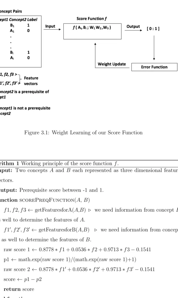
which should be labeled as 1 and the second instance is a prerequisite information fromAtoB which should be labeled as 0. The visual demonstration of the training data can be seen in the Figure 3.1.
For each prerequisite direction either from A to B or B to A, we are given three features and we need to make a prediction between 0 and 1. A suitable machine learning approach for this task is logistic regression, therefore, we apply it to come up with the best weights that would describe the prerequisite relations for all the pairs in the training data.
It is important to note that our classification accuracy and the training/test accuracy in logistic regression is different. To clarify this explanation it is best to look at a particular example:
Imagine that for a given concept pair (A, B) in the training data, the prerequisite relation from B to A is calculated as 0.4. Logistic regression classifies this as class 0 since it is less than 0.5 (more probable class) and it looks like we have a wrong classification because its true label is 1. Imagine also the prerequisite relation from
A toB is calculated as 0.3. It is classified as 0 and it is the true label. It seems like out of 2 examples we have only labeled one of them correctly but our classifier sees the (A, B) pair as a single example and it calculates the difference of the two scores and in that case, it is 0.4 - 0.3 = 0.1. Since 0.1 is a positive score it concludes that
B is a prerequisite of A therefore we have a correct classification for the concept pair (A, B).
After training our logistic regression model according to our training data, we deter-mine our weights to be: w1=0.8778, w2=0.0536 w3=0.9713 and w0=-0.1541. This finding suggests that the most important feature in the prerequisite calculation is the summary reference count, second is the RefD score and the last one is the article reference count. w0 can be thought of as a threshold value and it is found to be -0.1541 by our model.
The final structure of our prerequisite functionf is as follows:
3.1.4
Testing the Scoring Function
The prerequisite score function that we formulated can be used either as a regressor or a classifier. When used as a regressor, it predicts the strength of the prerequisite relation between the concepts A and B by outputting a score between -1 and 1 and when used as a classifier, it simply interprets the positive values as B being a prerequisite of A and the negative values as A being a prerequisite of B.
To test the performance, we use the function as a classifier to determine the accuracy in the test data.
Figure 3.1: Weight Learning of our Score Function
Algorithm 1Working principle of the score function f.
1: Input: Two concepts A and B each represented as three dimensional feature vectors.
2: Output: Prerequisite score between -1 and 1. 3: function scorePreqFunction(A, B)
4: f1, f2, f3← getFeaturesforA(A,B) . we need information from concept B
as well to determine the features of A.
5: f10, f20, f30 ← getFeaturesforB(A,B) . we need information from concept
A as well to determine the features of B.
6: raw score 1 ← 0.8778∗f1 + 0.0536∗f2 + 0.9713∗f3−0.1541 7: p1 ←math.exp(raw score 1)/(math.exp(raw score 1)+1)
8: raw score 2 ← 0.8778∗f10+ 0.0536∗f20+ 0.9713∗f30−0.1541 9: score ← p1−p2
10: return score 11: end function
make comparisons. The results obtained for this part will be explained in detail in Chapter 4.
3.2
Graph Formation
Now that it is possible to calculate a prerequisite score for any concept A and B
which have their corresponding articles in Wikipedia, we can go back to our initial goal of determining the prerequisite relations for a given set of concepts and then visualize this information by forming a graph out of it.
3.2.1
Prerequisite Matrix
Given a set of concepts C ={C1, C2, ..., Ck}We calculate each concept’s prerequisite
score with respect to the rest of the concepts and form the score matrixS.
S= s11 · · · s1k .. . ... ... sk1 · · · skk
where sij is the prerequisite score between the ith and jth concept.
Diagonal elements of the matrix are zero since the concept’s prerequisite relationship with itself is zero. Moreover sij = −sji because of the asymmetric property of our
function.
3.2.2
Matrix Filtering and Graph Building
The constructed score matrix needs to be turned into a graph for a visual represen-tation to the user and we explain the process in this subsection.
We use a graph database to store the concepts and their prerequisite information. A graph database is a database that uses graph structures for semantic queries with nodes, edges, and properties to represent and store data [19]. We choose Neo4j as the graph database management system which is developed by Neo4 Inc. According
to DB-Engines ranking [20], it is the most popular graph database. It has its own querying language called Cypher Query Language which is easy to understand and use and which also makes it possible to do complex graph operations in a few lines of codes. Moreover, any software written in any computer programming language can query the database using the Cypher Query Language through a transactional HTTP endpoint, or through the binary ”bolt” protocol [21].
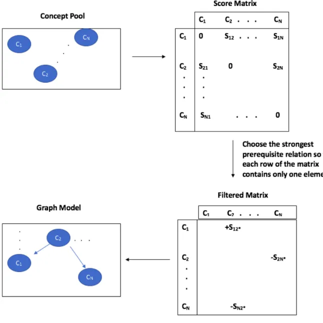
In our work, we treat each concept as a node in the graph and when we get the concept set C, we construct a node for every element in C. Then to be able to define the directed weighted edges we use the score matrix S.
Initially, the process seems rather straightforward and one can draw a weighted edge from conceptitoj if there is a positive scoresij and fromj toiif there is a negative
score sij. However, there are some issues to consider. The first issue is the possible
cycles in the graph. If conceptAis a prerequisite ofB, if conceptB is a prerequisite of C and if concept C is a prerequisite of A then the learner will be stuck in a loop in the graph and never proceed to the other concepts. To overcome this issue, we propose the following sparsification method:
For every concept ci in the concept list C, we look at the highest absolute value
scoresij∗by examining the i’th row of the score matrixS. This score demonstrates
the most powerful prerequisite relation for the concept ci. We only draw an edge
from the concept ci to concept cj∗ or vica versa according to the sign of the score
and discard the other scores in the i’th row of the matrix. We repeat the same procedure until there are no more concepts left in the concept list C.
This approach ensures an acyclic property in the graph. To prove this let’s analyze a simple case with three concepts A, B, and C with the random scores x, y, z. Imagine a score matrixS as follows:
S= 0 x z −x 0 y −z −y 0
toC meaning |y|>|x| and from C to A meaning |z|>|y|.
However, since |z| >|y| and |y| >|x|, the statement |z| >|x| should also be true. This contradicts with the assumption of |x| > |z| in the beginning so we are sure that we don’t have any cycles in the graph.
We should note that this algorithm only prevents cycle formation in the graph and other cases such as one concept being a prerequisite for multiple concepts or multiple concepts being prerequisite for a single concept is still possible.
Algorithm 2Graph construction algorithm 1: Input: List of concepts L
2: Output: Prerequisite concept graphG. 3: function buildScoreMatrix(L)
4: S ← createEmptyMatrix(size(L)) .creating an empty matrix with size
LXL
5: i← size(L) 6: j ← size(L)
7: for iteration 0 to i do 8: for iteration 0 to j do
9: S[i][j]← scorePreqFunction(L(i),L(j)) . filling the score matrix
10: end for 11: end for 12: return S 13: end function 14: function buildGraph(L,S) 15: for concept cin Ldo
16: createNode(c) . Create a node in the graph database 17: end for 18: i← size(L) 19: j ← size(L) 20: for iteration 0 to i do 21: temp← createEmptyList(size(L)) 22: for iteration 0 to j do
23: temp← S[i][j] . assign the scores in the same row to the list temp.
24: end for
25: value, index← getHighestAbsoluteValue(temp) . consider only the concept which has the highest absolute prerequisite score.
26: createEdge(L(i),L(index),value) .Create a weighted directed edge between these two nodes. Direction is decided according to the sign of the value.
27: end for 28: end function
3.3
Different Levels of Generalizations in the Graph
Often times we observe disconnected components in the graph since not every con-cept is a prerequisite of another concon-cept or some prerequisite relations are simply eliminated since they are not the strongest relations for that particular concept. These disconnected components are the natural clusters within the graph which may be seen as the higher level representations of the detailed content-specific concepts. One observation that we make from the high-school physics data-set is that concepts such as Velocity, Acceleration and Angular Velocity form one cluster in the graph which in fact belong to the topic of motion at a higher level.
Treating each cluster as a single node that generalizes some concepts at a higher level, we can in fact again use our algorithm to calculate a new score matrix S
and construct a new graph which contains higher level concepts. The procedure for doing that is rather straightforward and performed as follows:
Algorithm 3Graph generalization algorithm 1: Input: Graph G and Score matrix S.
2: Output: New graph G0 which is the one level higher version of the old graph
G .
3: Clusters←findClustersInGraph(G) . Clusters is a two dimensional list where each element contains the concept names that are in the same cluster. 4: function clusterLevelPrerequisiteScore(G1, G2)
5: sum← 0.
6: i← size(G1) . G1 is a list containing concepts in same cluster.
7: j ← size(G2) . G2 is a list containing concepts in same cluster.
8: for iteration 0 to i do 9: temp← empty list. 10: for iteration 0 to j do
11: weight← getWeight(G1(i),G2(j))
12: temp← weight
13: end for
14: value ←getHighestAbsoluteValue(temp)
15: sum← sum+ value
16: end for
17: return sum/size(G1)
18: end function
19: L0 ← assignLabels(Clusters) .Each cluster is in new list L0. 20: function buildHighLevelScoreMatrix(L0)
21: S0 ← createEmptyMatrix(size(L0)) . Empty matrix with size L0XL0
22: i, j ← size(L0) 23: for iteration 0 to i do 24: for iteration 0 to j do 25: S0[i][j]←clusterLevelPrerequisiteScore(L0(i),L0(j)) 26: end for 27: end for 28: return S0 29: end function
We have step by step explained our algorithms in three stages. In Chapter 4 we go over them once more by giving various examples from different stages and report our results in detail. We will be also analyzing our model’s performance on different data-sets and discuss its weak and strong aspects.
Chapter 4
Implementation, Experiments, and
Evaluation
In this chapter, we talk about experimental results performed to test our method-ology. We explain our methodology in three stages just like we did in Chapter 3 and we support our algorithm’s capabilities and efficiency at each stage by show-ing results obtained from different data-sets. There are three main different test data-sets:
1. An existing data-set that contains computer science topics labeled according to their prerequisite relationship.
2. A custom prepared data-set that includes database management system con-cepts.
3. High school physics concepts data-set that is again formed by us with the help of the existing online materials on the internet.
4.1
Prerequisite Score Accuracy
We first start our algorithm by constructing a function which computes a prerequisite score between -1 and 1 for two given concepts. The working principle of this function was explained in detail in Chapter 3 but it is important to make some remarks again so that what we are evaluating in this section becomes clear. Our function can both
serve as a classifier and as a regressor. In this section, we demonstrate its power in classification on various data-sets. Given two concepts A and B it can give either a positive or a negative score where positive means B is a prerequisite of A and negative means A is a prerequisite of B. If the score is exactly 0 then they are classified as NONE.
Before moving into the results, it is important to talk about the data-set format as well. The first test data-set is taken from [3]. It contains 154 pairs of computer science topics. All these concepts have corresponding articles in Wikipedia. For each pair (A, B) we are given the knowledge thatAis a prerequisite of B. If our function outputs a positive score it means it correctly classifies the given instance and if it gives a negative score it means it misclassifies the given instance. Moreover, since we also know the scores of our function for the test data-set, it is possible to calculate the error margin in the classification. In theory, we assume all the instances in the test data-sets are a full prerequisite of each other meaning that they should have a score of 1 if they are listed in a format of B is a prerequisite of A and -1 if they are listed as A is a prerequisite of B. We use the word in theory because in reality a concept is not always absolutely a prerequisite for another concept and rather it has a certain degree of prerequisite relation with it.
There is also another question on our mind before running the experiment on this data-sets. Since the function is trained with concepts from computer science, we want to know whether the domain similarity in the first data-sets adds any advantage to our function.
The function’s classification performance is also compared with the sole refD func-tion developed by Chen Liang and his team in 2015 [18]. This refD funcfunc-tion as we described earlier, was the starting point for us in determining a score function and we improved its performance by adding two new features and by learning the weights of these features with logistic regression on an existing training data. Out of 154 concept pair instances, 126 of them are correctly classified, and we obtained an accuracy of % 81 in the first data-sets. We then tested the sole refD method on the same test data but this time only 97 concept pair instances are correctly classified and the classification accuracy remained at % 63. Our method
outperformed refD by labeling % 18 more of the instances correctly. We analyzed the misclassified examples after the experiment and tried to identify the cause of this wrong classifications. One example pair from the first data-sets is Robotics and Robots. Our function states that robotics is a prerequisite for understanding robots but it is labeled other way around in the data-sets. This is rather an arguable instance and one can say to understand the robots we should study robotics or one can again say we should have knowledge about the term robot to study robotics. The other issue is the difference in the level of the concepts, for instance, if one concept is programming language and the other concept is C++, since C++ is a programming language it is not very accurate to look for a prerequisite relationship among these concepts because they rather have an isa relationship which is something different than what we are interested in..
By keeping the controversial instances in mind, we prepare our own data-sets which we believe is clearer than the other existing prerequisite data-sets. We first choose the domain to be high school physics concepts. There are two main reasons for choosing this domain. One is that like we stated above, we wanted to have a different area than computer science and secondly; it seemed easy to capture the prerequisite relations in physics. For instance, if we look at the definition of the concept Acceleration: the rate of change of velocity of an object with respect to time [22], one can easily understand that she has to first understand the concept
Velocity. It is also possible to look at the formulas for certain concepts in physics and state that the components of the formula for the given concept may be the prerequisites of it.
Our custom high school physics data-sets contains 82 concept pair instances. Out of 82 instances, 60 of them are labeled correctly with our function by reaching an accuracy of %73 while with the refD method only 46 of them are labeled correctly with an accuracy of %56.
Lastly, we move to our final data-sets which contains concepts from the database management system course. It is again a custom data-sets that is prepared by us. There are two main motives for choosing this course. Firstly in the former computer science topics data-sets, the concepts are not domain-specific and rather in general.
In this data-sets, we want to see the performance of the classifier when the concepts are in micro-level meaning that they are content-specific and short. Secondly, we are familiar with the course since my thesis advisor Y¨ucel Saygın is the professor of this course in our university and his expertise contributed to the data-sets preparation. Out of 50 database concept pairs, 33 of them are classified correctly with %66 accuracy and with refD method 27 of them are classified correctly with an accuracy of %54. The accuracy decreased but this was expected since there is a limited amount of information in Wikipedia about these detailed micro concepts.
4.2
Graph Formation
This is the second stage of our algorithm. Now for a given set of concepts C with lengthk, we are interested in forming n×n score matrixS where an element of the matrix sij is the prerequisite score between the concept iand concept j.
After forming score matrix S we are interested in turning this matrix into a graph structure in Neo4j where nodes in the graph represent the concepts and the directed weighted edges represent the strength and the direction of the prerequisite relations between concepts.
4.2.1
Complexity of the Algorithm
For a given set C with length n, we have to calculate each concept’s prerequisite score with the other concepts in the set, therefore, constructing the score matrix requires n2 operations. This complexity can be reduced to half by knowing the fact
that sij = −sji and sii= 0 in the score matrix S.
The main bottleneck for the algorithm is not the complexity of the calculations but rather the requests sent back and forth to the Wikipedia API. Each prerequisite score calculation for a concept pair (A, B) approximately takes 10 - 15 seconds because of the connection overhead. There may be several approaches to overcome this problem one is to parallelize the requests with multi-threaded programming. Another approach is to dump Wikipedia articles into the local machine in advance
to speed up the matrix formation process. Our length of the concept sets never exceeded 100, so we did not have much trouble because of this overhead.
4.2.2
Physics data-sets
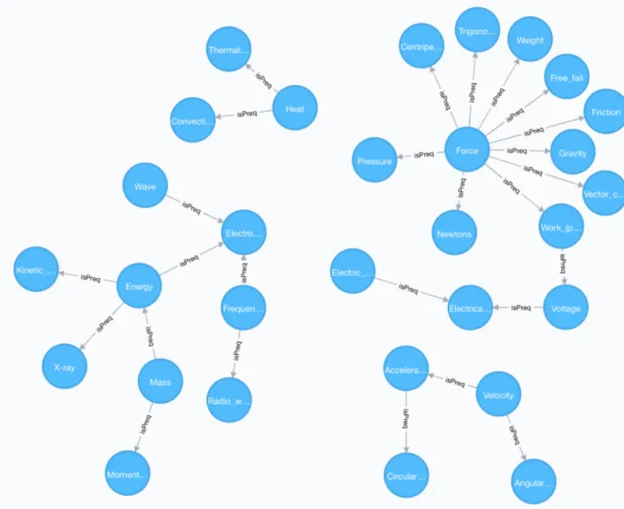
We first start with a set of 30 physics concepts and build their prerequisite graph.
Figure 4.1: General View of the Graph
The Figure 4.1 is the general view of the graph. We see four different clusters indicating those 30 concepts can be gathered around in four different categories. In the following figures, we zoom into the clusters and look at some individual prerequisite relationships found between concepts.
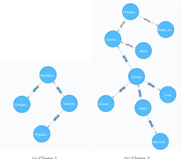
(a) Cluster 1 (b) Cluster 2 Figure 4.2: View of Cluster 1 and Cluster 2
forAcceleration andAngular velocity, andAcceleration is a prerequisite forCircular motion. Although not shown in Figure 4.2, it is possible to click the edges in the graph database and see the weights of each edge. The concepts in this cluster belong to a topic of motion at a higher level.
The second cluster has nine concepts inside. We observe that Mass becomes a prerequisite for Energy and Momentum. It makes sense as both of these concepts include mass in their formulas and if one does not know what mass is then she can not understand those concepts as well. Electromagnetic radiationrequires knowledge of the concepts Wave, Frequency, and Energy. These concepts in this cluster may belong to a topic of electromagnetic waves at a higher level.
In cluster 3, we see that Force is at the core of all concepts. Almost every concept requires knowledge from Force. Gravity, Friction, Weight and Pressure has the strongest prerequisite relationships withForce than the other concepts in the cluster.
(a) Cluster 3 (b) Cluster 4 Figure 4.3: View of Cluster 3 and Cluster 4
We should note that although for a given concept ci we only draw an edge to its
strongest prerequisite (or from its prerequisite to ci), we still don’t put a universal
threshold for the concepts in the graph. For example, an irrelevant concept may have a prerequisite relation to some concept ofA with weight 0.01 in the list and it may have zero prerequisite relationship with the others. In that case, that concept’s strongest prerequisite relation score is still 0.01 and we draw an edge for that relation. Our graph database provides an interface to any application-level service, therefore, it is possible to query the prerequisite scores of any concept pair in the graph. Furthermore, applications using our graph database can put their own thresholds if they want to filter out the weak prerequisite relations in the graph. For instance, applicationAcan state that the prerequisite scores below 0.5 will not be considered as meaningful relations or applicationB can take this threshold up to 0.8 etc. If the graph were to be constructed by a human expert, she would separate the concepts
Voltage,Electrical current andElectrical resistancebut our algorithm found a bridge concept Work which connects these clusters together. Indeed the definition of the
change in voltage is equal to the work per unit charge [23] and one should be familiar with concept Work before studying concept Voltage. The last cluster has three concepts inside and we see that conceptHeat is a prerequisite for the concepts
Convection and Thermal conduction which is an expected result.
4.2.3
Database Management System Concepts
In the second experiment, we give a set of 45 database management system concepts to our system. The general overview of the graph is presented in Figure 4.4
Figure 4.4: General View of the Graph
We observe again that similar concepts are gathered in the same clusters. There are six clusters, representing the topics of relational databases, concurrency control, data structures, database normalization, database recovery, and database indexing. We test some individual concept pair’s prerequisite scores by sending queries to our graph database to see if our graph is giving correct information or not.
MATCH ( n)−[ r : i s P r e q ]−>(m) where n . t i t l e =”P r i m a r y k e y ” and m. t i t l e =” F o r e i g n k e y ”
r e t u r n r . w e i g h t a s w e i g h t
We get a return value as : ”weight” 0.999759287115
Indeed concept Primary key is a prerequisite of Foreign key and we get a value very close to 1. It is important to note that weights are always positive and we understand the direction of the prerequisite by looking at the direction of the arrow or if we are writing a query, we specify it in theMATCH statement with the symbols (n)−[r :isP req]−>(m) where n and m are the concepts we are questioning, r is the type of the relation and−> symbol is the direction of this relation.
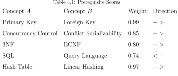
Here are some strong prerequisite relationships captured by our methodology in the graph :
Table 4.1: Prerequisite Scores
Concept
A
Concept
B
Weight
Direction
Primary Key
Foreign Key
0.99
−
>
Concurrency Control
Conflict Serializability
0.85
−
>
3NF
BCNF
0.80
−
>
SQL
Query Language
0.74
<
−
Hash Table
Linear Hashing
0.97
−
>
We hope that this graph becomes a helpful tool for the students who are interested in learning database management course. Although not implemented in this experi-ment, the Wikipedia links of the corresponding articles can easily be inserted inside the nodes so that the learner can immediately find the article and start studying.
4.3
Graph Generalization
In this section we refer again to the physics data-sets that is explained in Section 4.2.2. When we formed our graph for the 30 high school physics concepts, we
ob-served four different clusters each representing a different topic in the given context. We denote each cluster with the Ca,Cb, Cc, and Cd. Ca has the concepts regarding
the topics of Heat and Heat transfer, Cb has the concepts regarding the topic of
Motion Cc has the concepts of Energy and Electromagnetic waves, and Cd has the
concepts ofForce and Electricity. Below you can see each cluster with its concepts :
Cluster a={Heat, Convection, T hermal conduction}
Cluster b={Circular motion, Angular velocity, V elocity, Acceleration}
Cluster c={Kinetic energy, Radio W ave, M omentum, X–ray, Energy, W ave, F requency, Electromagnetic radiation, M ass}
Cluster d={T rigonometry, Electrical resistance, N ewton0s laws of motion, F orce, V ector calculus, F riction, P ressure, W eight, Centripetal f orce, F ree f all, V oltage, Electric current, Gravity, W ork}
According to the algorithm provided in Section 3.3 we should calculate each cluster’s prerequisite relation with other cluster and form the new prerequisite matrix S0. After the calculations we find the new matrix S0 to be :
S0 = 0 0.014 0.989 0.460 −0.005 0 −0.210 0.080 −0.184 0.263 0 −0.170 −0.150 0.312 0.148 0
Where the rows and the columns of the matrix are aligned according to order Ca,
Cb,Cc, and Cd.
One thing to note is that in the new matrixS0 we don’t have thes0ij =−s0jiproperty anymore because each cluster’s score with the other cluster is divided into its cluster size. In order to state a valid prerequisite relationship between any cluster i and
j, we seek the condition that if s0ij > 0 then s0ji < 0 or vica versa meaning that both clusters should agree about the direction of the prerequisite relationship or else they will be discarded. Assuming that a cluster pair agrees on the direction
of the relationship, to be able to calculate their score we perform the operation
k(s0ij −s0ji)k/2 to come up with the final weight score.
Continuing with our example, we analyze the new score matrix S0 and at each row, we pick the highest absolute value.
For the cluster Ca, the highest absolute value in its row is 0.989, therefore, Cc is a
prerequisite ofCaand we should draw an edge fromCctoCa. For the clusterCb, the
highest value in its row is -0.21 hence Cb is a prerequisite of Cc and we should draw
an edge fromCbtoCc. For the third row, we observe thatCc’s strongest prerequisite
isCb and we again draw an edge fromCb toCc. For the last row we observe thatCb
should be a prerequisite of Cd with the highest value being s0db = 0.312. However,
s0bd = 0.08 is also positive meaning that there is not a clear agreement between the direction of the prerequisite relationship, therefore, we leave cluster d out.
We calculate the weights as: :
k(−0.210−(0.263))k/2 = 0.473 for the edge Ebc.
k(0.989−(−0.184))k/2 = 0.586 for the edge Eca
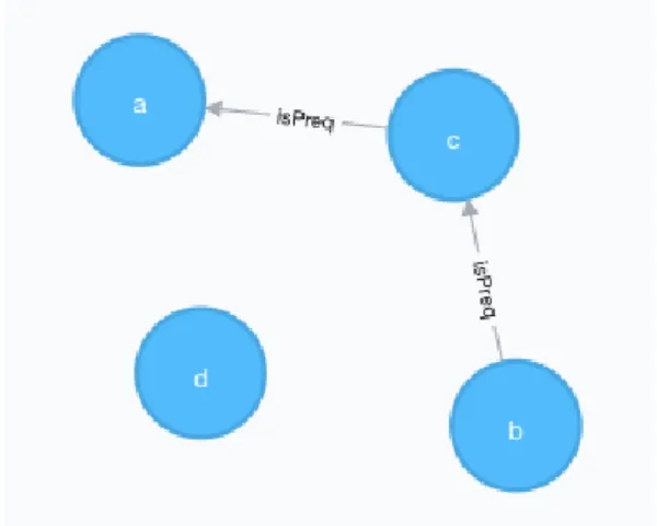
Now the second level graph is formed as shown in Figure 4.5 :
Figure 4.5: Second Level Physics Graph
Observing Figure 4.5 we conclude that topic speed and motion (Cb) is a
prerequi-site for the topic energy and electromagnetic waves (Cc) and the topic energy and
electromagnetic waves is a prerequisite for understanding the topic heat and heat transfer (Ca).
Now the second graph can be further divided into two new clusters C1 and C2. In C1 there are former clusters Ca, Cb, Cc and in C2 there is only Cd. It is possible
to re-do the procedure above to determine if there is any prerequisite relationship between the clusters by observing the matrix S’. Since C1 has only the topic Cd,
the element with the largest absolute value in the last row of S’ will determine the prerequisite score from C2 to C1 which is 0.312. For calculating a score from C1
to C2, we consider each elements (Ca, Cb, Cc) prerequisite score withCd which are
0.460, 0.08 and -0.17 respectively. Summing these values up and dividing them to the size of C2 yields a score of 0.123. Since both of these scores are positive we conclude that they do not agree on the direction of the prerequisite relationship and we do not assign a prerequisite relation between the clusters.
Although not considered in our methodology, if the user wants to force prerequisite relationships between clusters and does not want to see any left out clusters in the graph she can do the following: If clusterci and cj have both negative scoressij and
sji, it implies that cluster ci is a prerequisite of cj and cluster cj is a prerequisite
of ci. In that case, we can simply pick the cluster which has the score with the
maximum absolute value and draw an edge from that cluster to the other cluster. We can calculate the weight score as k(s0ij −s0ji)k/2. If cluster ci and cj have both
positive scores sij and sji, this time it implies that cluster cj is a prerequisite for
cluster ci and cluster ci is a prerequisite for cluster cj. In that case, we can pick
the cluster which has the score with the maximum absolute value and draw an edge from that cluster to the other cluster. The weight determination is same in both cases with the operationk(s0ij−s0ji)k/2. This approach creates an alternative graph that does not contain any disconnected components.
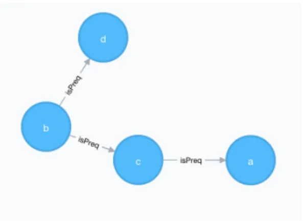
When we perform this alternative algorithm to our example in the second level graph,Cb is a prerequisite forCdwith a score of 0.312 and clusterCdis a prerequisite
for Cb with a score of 0.08. We consider the score with the highest absolute value
which is 0.312, therefore, we conclude that Cb is a prerequisite for cluster Cd. We
calculate the weight as k(0.312−0.08))k/2 = 0.116 and we conclude that Cb is a
prerequisite for clusterCdwith a prerequisite score of 0.116. Our alternative second
Figure 4.6: Second Level Alternative Physics Graph
In our alternative graph, the learner can have two preferences. If she wants to master concepts regarding heat and heat transfer (Ca) she first needs to master the
concepts of motion (Cb) and then master the concepts of energy and electromagnetic
waves (Cc) and then start learning topic Ca. Alternatively, if the learner wants to
master the whole context (all of the topics in high school physics) she should start with topicCb, then she can study topicsCcand Cdand then she can study the topic
Ca to finish the given graph.
The constructed graph is aimed to serve the learner as a tool to facilitate her learning process. The graph can be enriched in many ways and we believe it has the potential to increase student performance in lots of different courses. These ideas and possible future applications of these prerequisite concept graphs are discussed in Chapter 5.
Chapter 5
Conclusion and Future Work
In the quest of finding an organized representation of the huge unstructured on-line learning materials, we believe that the concept prerequisite graphs constructed through our methodology will guide the learners in their learning process. We also provide an extendable framework on top of which many more innovative ideas can be developed.
The prerequisite score calculations are currently based on the articles on Wikipedia. We use three main features in prerequisite score calculation but there can be other important features that may contribute to prerequisite scores as well. For instance, one can also include the reference position of the concept in the article as a new feature or one can consider the size of the article when calculating the reference feature and so on. With the addition of the right features, we think the classification performance of our system may be further increased.
We choose to seek the concepts in Wikipedia because of its useful properties that we mentioned throughout the thesis but it is also possible to incorporate knowledge from other resources to calculate prerequisite scores. Those resources can be video as well as text-based.
In the graph construction algorithm, we always include a concept’s strongest pre-requisite in order to avoid possible cycle formations. However, there may be an alternative algorithm where not only the strongest prerequisite but also multiple strongest prerequisites may be used while still preserving the acyclic property of the graph. In Section 4.2.2 we mention a universal threshold that each prerequisite
score needs to pass. In our work, we don’t have this kind of threshold. However, with various experiments on large data-sets it may be helpful to come up with such a threshold which can guarantee that there are no weak prerequisite relations in the graph.
Besides the algorithmic part, if we go back to our initial objective of enhancing student learning experience there can be several components in the graph that may help the students. For example, a questioning component may be added to the graph. Each node in the graph may be enriched with multiple questions regarding its concept. If the student wants to move on to another concept that the current concept is a prerequisite of, she may have to correctly answer the questions of that concept so that we understand that the student fully grasped the content in that topic. Since each node is, in fact, a Wikipedia article, the nodes can also include links to these articles. Furthermore, for the same topic there can be multiple different resources so that if a student does not understand the article, she may move to the alternative resources.
Once the graph is formed, it is stored in a graph database and it can be implemented as a web service to other systems. An intelligent adaptive learning management system may use this database to present learning paths to students according to their objectives. By keeping track of each student’s profile and the past data, the intelligent system can change the weights of the edges if it thinks there are other alternative prerequisite relations based on the student data it has.
The domain invariant property of the algorithm makes the system a useful learning tool not just for computer science, and physics courses but for other courses from other domains. We believe that especially the students studying courses that require lots of reading and domain- specific terminologies such as biology or literature will benefit most from our system.
Appendix A
Tabular results of evaluations on
each data-set
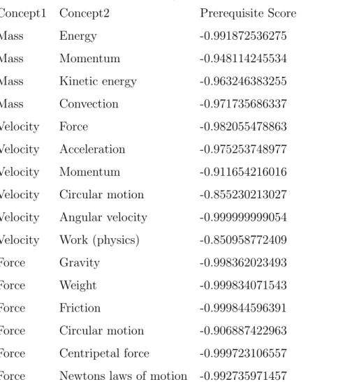
Table A.1: Evaluations on physics data-set with a threshold value of 0.8. Concept1 Concept2 Prerequisite Score
Mass Energy -0.991872536275
Mass Momentum -0.948114245534 Mass Kinetic energy -0.963246383255 Mass Convection -0.971735686337 Velocity Force -0.982055478863 Velocity Acceleration -0.975253748977 Velocity Momentum -0.911654216016 Velocity Circular motion -0.855230213027 Velocity Angular velocity -0.999999999054 Velocity Work (physics) -0.850958772409 Force Gravity -0.998362023493
Force Weight -0.999834071543
Force Friction -0.999844596391 Force Circular motion -0.906887422963 Force Centripetal force -0.999723106557 Force Newtons laws of motion -0.992735971457
Table A.2: Evaluations on physics data-set with a threshold value of 0.8.
Concept1 Concept2 Prerequisite Score
Force Work (physics) -0.999915440679
Force Free fall -0.954538589358
Force Pressure -0.988458568502
Acceleration Circular motion -0.972457410798
Energy Friction -0.99901259911
Energy Heat -0.999996465462
Energy Thermal conduction -0.997922157957
Energy Kinetic energy -0.99999601306
Energy Electromagnetic radiation -0.99999728113
Energy X-ray -0.921038883094
Energy Wave -0.916567809217
Gravity Free fall -0.938609274061
Friction Work (physics) 0.800898909263
Friction Kinetic energy 0.88966442389
Heat Thermal conduction -0.999998584781
Heat Work (physics) 0.999889373899
Heat Convection -0.999999795139
Frequency Electromagnetic radiation -0.999920774246
Work (physics) Voltage -0.821566035606
Table A.3: Evaluations on database management systems data-set with a threshold value of 0.5.
Concept1 Concept2 Prerequisite Score
Entity relationship model Relational database 0.574905971913
Database design Foreign key -0.917743478419
Database design Database normalization -0.810222201105
Primary key Foreign key -0.999759287115
Primary key Weak entity -0.99643657114
Foreign key SQL 0.933692406412
Foreign key Weak entity -0.821307950347
Foreign key Stored procedure 0.529595722782
SQL Query language 0.74519392494
SQL Stored procedure -0.846331854774
1NF Relational database 0.808997494714
3NF BCNF -0.801929651851
ACID Database transaction -0.515820232241
Atomicity (database systems) Write ahead logging -0.530019702361
BCNF Functional dependency 0.794670233574
Concurrency control Conflict serializability -0.852474283314 Concurrency control Multiversion concurrency control -0.978476116184 Concurrency control Optimistic concurrency control -0.989795078295 Concurrency control Timestamp-based concurrency control -0.822766390581 Concurrency control Two phase locking -0.555309700087 Database normalization Functional dependency -0.538208598348 Database normalization Relational database 0.557931828985 Functional dependency Relational database 0.523605637531
Hash table Linear hashing -0.975295097481