Citation: Xu, Shoujiang, Ho, Edmond S. L. and Shum, Hubert P. H. (2019) A hybrid metaheuristic navigation algorithm for robot path rolling planning in an unknown environment. Mechatronic Systems and Control, 47. p. 46072. ISSN 1925-5810
Published by: Acta Press
URL: https://doi.org/10.2316/j.2019.201-3000 <https://doi.org/10.2316/j.2019.201-3000> This version was downloaded from Northumbria Research Link: http://nrl.northumbria.ac.uk/35636/
Northumbria University has developed Northumbria Research Link (NRL) to enable users to access the University’s research output. Copyright © and moral rights for items on NRL are retained by the individual author(s) and/or other copyright owners. Single copies of full items can be reproduced, displayed or performed, and given to third parties in any format or medium for personal research or study, educational, or not-for-profit purposes without prior permission or charge, provided the authors, title and full bibliographic details are given, as well as a hyperlink and/or URL to the original metadata page. The content must not be changed in any way. Full items must not be sold commercially in any format or medium without formal permission of the copyright holder. The full policy is available online: http://nrl.northumbria.ac.uk/policies.html
This document may differ from the final, published version of the research and has been made available online in accordance with publisher policies. To read and/or cite from the published version of the research, please visit the publisher’s website (a subscription may be required.)
Manuscript received 30 Novermber 2017
For the Special Issue of Drs. Gelan Yang, Tahir Khan et al.
A HYBRID METAHEURISTIC NAVIGATION
ALGORITHM FOR ROBOT PATH ROLLING
PLANNING IN AN UNKNOWN ENVIRONMENT
Abstract
In this paper, a new method for robot path rolling planning in a static and unknown environment based on grid modelling is proposed. In an unknown scene, a local navigation optimization path for the robot is generated intelligently by ant colony optimization (ACO) combined with the environment information of robot’s local view and target information. The robot plans a new navigation path dynamically after certain steps along the previous local navigation path, and always moves along the optimized navigation path which is dynamically modified. The robot will move forward to the target point directly along the local optimization path when the target is within the current view of the robot. This method presents a more intelligent sub-goal mapping method comparing to the traditional rolling window approach. Besides, the path that is part of the generated local path based on the ACO between the current position and the next position of the robot is further optimized using particle swarm optimization (PSO), which resulted in a hybrid metaheuristic algorithm that incorporates ACO and PSO. Simulation results show that the robot can reach the target grid along a global optimization path without collision.
Key Words
Robot Path Rolling Planning, Ant Colony Optimization, Particle Swarm Optimization, Local Navigation Path
1. Introduction
2
significant achievements of mechanical and electrical integration. In particular, finding a safe path for the robot from the starting point to the target point of a working environment with obstacles is an important research area in mobile robotics [1], which is an NP-Hard problem. According to the working environment, the path planning model can be divided into two major categories, namely, model-based global path planning in which information of the operating environment is known, and sensor-based local path planning in which operating environment information is fully or partial unknown [2]. This paper focuses on robot path planning in an unknown environment.
Robot path planning methods consist of classic and heuristic approaches. Classic algorithms are usually computationally more expensive, such as the roadmap approach [3], Voronoi diagram [4], potential field [5], and cell decomposition [6]. Heuristic approaches are particularly useful when the environment is more complex, and have shown good results in overcoming the limitations of traditional methods. Representative methods include the A* algorithm [7], simulated annealing [8], rapidly-exploring random tree [9], genetic algorithm (GA) [10], fuzzy logic [11], artificial immune algorithm [12,13], ant colony optimization (ACO), etc. In particular, first developed for solving the travelling salesman problem, ant colony optimization has been heavily used in robot path planning because of its superiority in path planning [14]. [15] presented a modified ACO algorithm for global path planning. The simulation results show that it could generate an optimal path based on grid modelling. Compared to some other algorithms, ACO is preferred in robot path planning. In particular, the ACO algorithm is more effective and less costly than the A* algorithm and the genetic algorithm, especially when the grids within the robot’s view become larger. Also, the average path length obtained by the rapidly-exploring random tree method is much longer than that of the ACO algorithm. Meanwhile, the combination of different intelligent algorithms becomes more and more popular. [16] proposed a novel algorithm relying on potential fields and genetic algorithms to overcome their inherent limitation and effectively plan out a global optimization path in different complex scenarios. [17] presented an efficient
3
hybrid ACO-GA algorithm for global path planning. It can improve the solution quality by relying on the combination of the ACO and GA advantages.
In an unknown environment, the robot can only obtain obstacle information within the robot’s view through the sensor, and constantly utilizes and dynamically feedbacks the information within the robot’s view to plan a local navigation path. Rolling window is an effective method for robot path planning in unknown environments. [18] proposed an adaptive artificial potential field method combined with the rolling window method to solve the local-minima problem and plan the robot path in a dynamic environment. [19] proposed a new robot path rolling planning algorithm which maps the goal node to a sub-goal node nearby the boundary of robot’ view. [20] presented a novel and effective robot path planning method for dynamic unknown environments. In each iteration, the robot planned a local navigation path based on an improved ant algorithm. The idea of the traditional rolling window method [18, 19, 20] is relatively simple, lack of intelligence and only incorporate the global target information into the sub-target selection, instead of combining it with the holistic environment information in the robot’s view. The traditional rolling windows approach maps the sub-target point to the boundary of the planning window, and the sub-target point guides the robot to the target point. As the purpose of guiding the robot towards the target point is too intensified, the planned path is often subject to detours and is not a globally optimal one. Meanwhile, it is very easy to fall into local deadlock and oscillation.
In this paper, we propose an algorithm such that in a condition where the robot does not know all obstacles in advance, it can ensure the robot to reach the target safely in a static and unknown environment. The contributions of this paper can be summarized as follows:
A robot path rolling planning algorithm based on ACO (RPRP_ACO) is proposed, which combines
the environment information of the robot’s view and target point information to effectively plan the local navigation path.
4
path rolling planning algorithm (RPRP_HYBRID) is formed.
This paper is organized as follows. In Section 2, the modelling of the static and unknown working environment and the robot’s view is defined. Section 3 introduces the proposed RPRP_ACO algorithm and the related definitions. Section 4 further describes the RPRP_HYBRID process. Section 5 presents the experimental results to evaluate the two proposed algorithms. Conclusions are drawn in Section 6.
2. Environment Modeling
In this section, the working environment of the robot will be modelled. Assuming that there is a finite number of unknown and static obstacles ob1, ob2, ..., obn in a 2-dimensional working area (WA), the
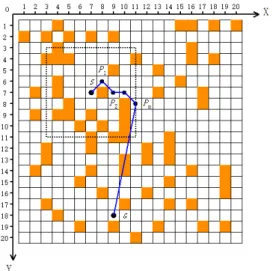
purpose of the robot path planning is to reach the target point G from the starting point S along a safe, collision-free and optimized path. The robot can detect environment information in the view domain (VD) at any time. The WA is quantized by dividing the space into grids and the obstacle obi (i = 1, 2, ..., n) will fill an individual grid. The Cartesian coordinate system XOY which vertical axis is Y and horizontal axis is X is being used in the WA. Fig. 1 shows an example WA with orange-colored grids occupied by obstacles and the free space are indicated by blank grids. Each grid g has a corresponding coordinate value (x, y), denoted by g (x, y) where x is the column number, and y is the row number. In Fig. 1, the starting point S of the robot is(7, 7), the target point G is (9, 18), the radius of VD is 4, and the VD indicated by the size of the dotted line is 9 × 9. At any time, the robot can only walk directly to one of its adjacent free grids. For example, the accessible grids for the robot are limited to the set {(6,6), (7,6), (8,6), (6,7), (6,8), (7,8), (8,8)} when the current position is S.
5
Figure 1. Environment Modelling
3. Robot Path Rolling Planning in a Static and Unknown Environment 3.1 Methodology and Related Definition
We formulate this robot path planning in an unknown environment based on the assumptions that have been widely used in the literature. Specifically, only limited information is available to the robot, including the environment information in its view VD and the position information of the target point G at the initial point S. An example of finding a collision-free path between S and the boundary point Pm in VD is illustrated in Fig. 1. The robot moves forward by step λ according to the path and reaches a new location point, and re-plans the local optimization navigation path in a new rolling window. To make the robot moves along a better-optimized path to the target point G, each scheduled local navigation path should be collision-free and possess a near minimum value of f (Pm) + h (Pm), where f (Pm) represents the distance
from the current robot’s position to the boundary point Pm of the view, and h (Pm) is the cost estimation of
the path from Pm to the target point G. To simplify the calculation, h (Pm) is estimated by the distance
between the point Pm and the target point G, since information outside the robot’s view is not available.
Ant colony optimization simulates ant colony behaviour to find the best foraging strategy from the nest to the food source. By placing a group of ants at the current location of the robot, the ants collaborate with each other within the robot’s view VD to find the best local navigation optimization path. During the path planning process, these steps will be repeated when the robot reconstructs a new navigation path by using
6
the ant colony algorithm based on the information in a new VD. When the target point G is in the robot’s view, the robot will move to the target grid directly along a path computed by local optimization. By this, the robot will be guided by each optimal navigation path to move from the starting to the target point along a global optimization path.
To facilitate the description of the algorithm, as defined below:
Definition 1: After the WA is modelled as grid cells, the number of grids per row is denoted by NX, and
the number of grids per column is denoted by NY.
Definition 2: The ith grid is denoted by gi (i = 1, 2, ..., NX × NY), the corresponding abscissa value x is
calculated from equation (1), and the ordinate value y is calculated according to equation (2):
1 N 1)mod (i x = − x + (1) 1 ) 1)/N (int)((i y = - x + (2)
The grid set containing all gi is denoted by GS. The set consisting of all i is denoted by NS.
Definition 3: The set of grids occupied by the obstacle obi (i = 1,2, ..., n) is denoted by OS. Any gi satisfying gi ∈GS and gi ∉OS is called an accessible point, and the set of all accessible points in the environment is called an accessible domain, denoted by AD. Particularly, the accessible domain within the robot’s view VD is denoted by VAD.
Definition 4: The distance between grid gi and grid gh is denoted by d (gi, gh), and the formula is:
2 h i 2 h i h i,g ) (x x ) (y y ) d(g = − + − (3)
If gi and gh are adjacent grids, the connection between the two grids is called an edge eij whose distance
d (gi, gh) is 1 or 2.
Definition 5: The current grid of the robot is denoted by gR. The current view of the robot is denoted by
VD (gR), and the accessible domain VAD within the view VD is denoted by VAD (gR).
7
and Tij(t) represents the pheromone on the edge eij at time t, where i , j∈NS.
Definition 7: The antk’s state during the foraging process is denoted by Statek. The three different ant states are death, foraging and forage-completed respectively and their corresponding Statek values are -1, 0, 1.
Definition 8: Tabuk denotes the set of grids antk passed in a planning process, whose elements are represented as Tabuk
1, Tabuk2, ..., TabukN (k), where N (k) is the number of grids in Tabuk. Particularly, when
Statek value is 1,the grids in the Tabuk represents a local navigation path from the starting point to the
target point.
Definition 9:BRR(gi) represents the neighbor domain of grid gi in the view VD (gR), where BRR(gi) ={ gj | d(gi,gj)<= 2, gj∈VAD (gR)}.
Definition 10: The step size λof the robot represents the total number of the grids which the robot passes through along a navigation path in a rolling window.
3.2 Robot Path Rolling Planning Based on Ant Colony Optimization
Having presented the environment modelling, the principle and definition of the algorithm in the last section, the robot path rolling planning based on ant colony optimization (RPRP_ACO) are described as follows:
Step 1: Generating an arbitrary starting point S and a target point G in the accessible domain AD of the environment WA (the gR point is the same as the S point at the beginning), and initializing the related
parameters of the ACO.
Step 2: If the current position gR and the target point G are the same, the planning process is finished;
otherwise go into Step3.
Step 3: The robot detects the environment information at the current position gR to obtain grids
information in the robot’s view VD (gR), and records the coordinate of each obstacle obi and the free nodes in the accessible domain VAD (gR).
8
Step 4: The iteration accumulator I is 0 and the maximum number of iterations is MAX. Initialize the pheromone τij(0) as τ0(τ0is a constant) on the edge eij formed by two free adjacent nodes in the accessible domain VAD (gR).
Step 5: Place m ants at the current position point gR and add the number R into the Tabuk (k = 1, 2, ..., m). The number N (k) of the Tabuk is set to 1. Initialize Statek value as 0.
Step 6: For any antk, if its Statek value is 0, select a node gj based on its current grid gi according to the following selection strategy and add the number j to Tabuk, and the N (k) value is automatically incremented by 1. If BRR(gi)is empty, update Statek value as -1 and the current antk stop searching. Selection strategy: generate a random number q in (0,1), if q is less than q0 (q0 is a predefined
threshold and 0 < q0 <1), then select the grid j by equation (4), otherwise by equation (5), where j,s∈
BRR(gi) and j,s∉Tabuk are satisfied:
} (t)] [η (t)] max{[τ arg j = ij α ij β (4)
∑
= β is α is β ij α ij ij k (t)] [η (t)] [τ (t)] [η (t)] [τ (t) Pro (5)where t denotes the ant foraging time, α denotes the relative importance of the pheromones on the trajectory, β denotes the relative importance of the edge eij and ηij(t) is the heuristic information. To
simplify the calculation, we define the heuristic functionηij(t)is equal to 1/d(gi,gj). The probability that antk moves from gi to gj at time t is represented by Prokij(t).
Step 7: Local pheromone update rule. Local pheromone update is carried out by each ant in the process of establishing a solution, and ρ is the pheromone evaporation coefficient. Each ant chooses a node, and the pheromone between the two grids is updated according to formula (6):
k ij ij
ij(t 1) (1 - ρ)τ (t) ρΔτ
9
when τij(t +1)<τmin,set τij(t + 1)=τmin;when τij(t +1)>τmax,setτij(t + 1)=τmax. k
ij
τ
∆ is equal toQ1/
lk if the antk passed the edge eij, otherwise is set to 0. lk is the length of the path that antkhas traveled in this foraging process, and its value is the sum of the distances between two adjacent points in Tabuk, calculated by equation (7):
∑
− = + = N(k) 1 1 i Tabu Tabu k d(g , g ) l i 1 k i k (7)Step 8: Depending on whether the target point G is in VD (gR), there are two cases to consider whether
the antk has finished foraging.
Case 1: If G is not included in VD (gR), and grid (k) k
TabuN
g in the Tabuk belongs to the boundary of the robot’s current view, the ant will be considered to complete the path search. the target point G will be added to the Tabuk, N (k) automatically add 1, and Statek value is set to 1.
Case 2: If G is included in VD (gR), and the last element TabukN (k) of the Tabuk is the target point G, the ant is considered to complete the path search, and the Statek value is set to 1.
Step 9: For all ants, if all the Statek values are nonzero, then go to Step10, otherwise go to Step6. Step 10: Depending on whether the target point G is in VD (gR), the best path lmin is calculated in two
cases.
Case1: If G is not included in VD (gR) and the Statek value of the antk is 1, the length is calculated by (8): )) g , h(d(g ) g , d(g l N(k) k 1 N(k) k 1 i k i k Tabu Tabu 2 N(k) 1 i Tabu Tabu ' k =
∑
+ + − − = (8)To simplify the calculation, we seth(d(g , g )) d(g , g N(k) )
k 1 N(k) k N(k) k 1 N(k)
k Tabu Tabu Tabu
Tabu − = − .
Case2: If G is included in VD (gR) and the Statek value of the antk is 1, the length is calculated according to (7).
10
Step 11: Global pheromone update rule. According to the grids of the best path, the pheromone information on the edge eijformed by the adjacent grids is updated by equation (9):
ij new ij new ij (1 u)τ uΔ τ = − + τ (9) where
∑
= ∆ = ∆ m k k ij ij 1 ττ , u is the global pheromone evaporation coefficient, and ∆τijk=Q2/lmin if eijwhich
antk passed belongs to the best path, otherwise is equal to 0.
Step 12: The number of iterations I is automatically incremented by 1, if I is not equal to MAX, then clear the Tabuk, go to Step5 and repeat the foraging process until I is equal to MAX. The best path in the final memory of robot is the local navigation path.
Step 13: If G is not included in VD (gR), the robot moves forward along the planned local navigation path by step λ, and the robot goes to a new coordinate position, updates the gR point, and returns to Step2
to repeat the process. If G is included in VD (gR), the robot travels to the end-point G along the best path.
4. Robot Path Rolling Planning Based on Hybrid Heuristic Algorithm
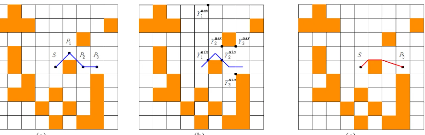
A local navigation path is planned based on the above RPRP_ACO algorithm in each rolling window. According to the step size λ, the next position of the robot can be calculated. Due to the drawbacks of the grid modelling, the path between the current position and the next position can be further optimized. To solve this problem, here we propose an RPRP_HYBRID algorithm to optimize the path between the two positions based on particle swarm optimization. In Fig. 1, the path from S to G is the local navigation path planned by RPRP_ACO. For example, assuming that the step size λ is 3, the next robot location will be P3.
Our purpose now is to optimize the path between the point S and point P3 using particle swarm
optimization, as shown in Fig. 2(a). Notice that when the step size is 1, the path between the current position S and the next position P1 cannot be further optimized. The concrete steps of the algorithm are as follows:
11
(a) (b) (c)
Figure 2. The illustration of a local navigation path optimized by particle swarm optimization. Notice that the path touching the obstacle does not mean any collision. (a) A part of the local navigation path. (b) The
vertical searching space of each cross point. (c) The path further optimized by PSO.
Step 1: Obtain the local navigation path between the current position gR and the next robot location
Pλbased on the RPRP_ACO algorithm.
Step 2: Calculate the number of intersection points of the path and the vertical lines. Assuming the number of crosspoints is NUM, then the vertical searching space of the dth cross point belongs to (Ydmin,
Ydmax), 1<=d<=NUM, as shown Fig. 2(b). The dthhorizontal coordinate of the cross point is denoted by Xd. Step 3: Initialize the parameters of particle swarm optimization, the initial locations and velocities of all particles. The number of the particles is PN, and the best location Yibest of the ith particle is initialized as its initial location. The maximum and minimum inertial coefficients are denoted by Wmax, Wmin
respectively. ω is inertial coefficient and ω= Wmax. C1 and C2 are acceleration coefficients. Set the
maximum of the iteration as Imax, and the current iteration is IC initialized as 0.
Step 4: Calculate the fitness F(Yi(t)) of each particle i based on equation (3) and equation (10), and the particle with the best fitness is denoted Yg. The fitness function F(Yi(t)) is:
) λ P ), Y , d(g(X )) Y , g(X ), Y , d(g(X )) Y , g(X , d(g (t))
F(Y NUM i,NUM
1 NUM 1 d 1 d i, 1 d d i, d i,1 1 R i = +
∑
+ − = + + (10)Step 5: Update the velocities and positions of all particles according to the equation (11) and equation (12): (t)) Y (Y r C (t)) Y (Y r C (t) ωV 1) (t V i,d d , g 2 2 d i, best d i, 1 1 d i, d i, + = + − + − (11)
12 1) (t V (t) Y 1) (t Yi,d + = i,d + i,d + (12)
If Yi,d< Ydmin ,then Yi,d= Ydmin; if Yi,d < Ydmax, then Yi,d= Ydmax. r1, r2 are random values (0<= r1, r2<=1).
Step 6: Update the Yibest and Yg according to every particle’s fitnessF(Yi(t)) calculated by equation (10).
IC = IC +1, ω= (Wmax– (Wmax– Wmin)* IC) / Imax. Step 7: If IC < Imax, then go to Step5.
Step 8: The path (gR, g(X1, Yg,1), g(X2, Yg,2), …, g(XNUM, Yg,NUM), Pλ) is the final path the robot will follow by in a rolling window, which is shown Fig. 2(c).
5. Simulation Results
In this section, we present the experimental results for evaluating the effectiveness and robustness of the proposed algorithms. All the experiments were running on a computer with an Intel Core i7-7500U 2.90 GHz GPU and 4GB of RAM. The algorithms were implemented in C# with Visual Studio 2015. The
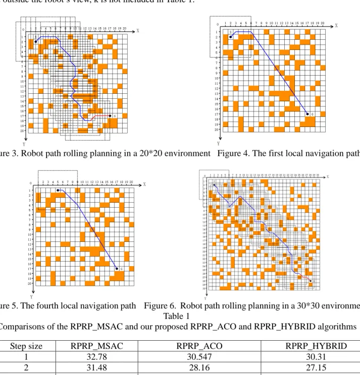
parameters of the algorithm for all simulations are set as the following. ACO: m=20, MAX=200, α=1, β=2, q0=0.7, ρ= u=0.8, Q1= Q2=100; PSO: PN=40, Wmax=0.9, Wmin=0.4, Imax=500, C1= C1=2.0. Fig. 3 shows the process of robot path rolling plan in a 20 * 20 environment. The robot step λ is 1, the radius and size of robot’s view are 4 and 9 × 9, respectively. When the robot advances to point (13, 18), the target point G enters the robot’s view, and the planned path is indicated in red. The final path length is 30.97 and the number of rolling windows is 23. In this environment, the robot can effectively plan a real-time optimization path from the starting point to the target point. Fig. 4 shows the robot plans out the first local navigation path based on the ant algorithm at the starting point S, and Fig. 5 is the fourth local navigation path. In Fig. 3, if the traditional rolling window method [18, 19]is utilized, its sub-target will be mapped at (6,6), resulting in the inability to plan a valid local navigation path.
The number of grids on local navigation paths of the RPRP_ACO algorithm is greater than or equal to the radius 4 of the robot’s view, and the number of local navigation path nodes may be different each run time. To facilitate comparison, the step size is limited in an array {1,2,3, k}, where the step k indicates that
13
the robot moves directly to the sub-target point along each local navigation path in each rolling window, and is a dynamically changing value. The robot path rolling planning based on MSAC algorithm (RPRP_MSAC) proposed in paper [20] can generate an optimal path in the environment of Fig. 3, and Table 1 shows the comparison of the average path length of 10 runs with three different step sizes among RPRP_MSAC and the two proposed algorithms. As the RPRP_MSAC algorithm maps the sub-goal to a grid outside the robot’s view, k is not included in Table 1.
Figure 3. Robot path rolling planning in a 20*20 environment Figure 4. The first local navigation path
Figure 5. The fourth local navigation path Figure 6. Robot path rolling planning in a 30*30 environment Table 1
Comparisons of the RPRP_MSAC and our proposed RPRP_ACO and RPRP_HYBRID algorithms
Step size RPRP_MSAC RPRP_ACO RPRP_HYBRID
1 32.78 30.547 30.31
2 31.48 28.16 27.15
14
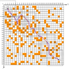
To further demonstrate the effectiveness of the RPRP_ACO algorithm, Fig. 6 shows the robot path planning process in a 30 * 30 random environment. The ratio of free grids to barrier grids is 1: 4, the robot step size is 2, the final planned path length is 45.70, and the number of rolling windows is 18. Fig. 3 and Fig. 6 show that the robot can intelligently avoid the trap area. If the PSO is further integrated into the RPO_ACO planning process and the RPRP_HYBRID algorithm is formed. Then the final planned path length for the environment of above Fig. 6 is 43.97, as shown in Fig. 7. For the environment of Fig. 6, when the robot moves along the local navigation path to the sub-target each time, the comparison of the paths planned by the two proposed methods are shown in Fig. 8, the blue path is planned by the RPRP_ACO, and the red path is planned by the RPRP_HYBRID. The length of the two paths are 50.11, 46.30 respectively and the number of rolling windows is 10.
Figure 7. The final path planned by RPRP_HYBRID Figure 8. Comparison of the two paths For the environment in Fig. 6, the average path length and the average number of rolling windows of 10 successive runs obtained by the two approaches with different step sizes are shown in Table 2. It shows that the path length obtained by the RPRP_HYBRID algorithm is more optimal, and when the robot step size is 2 the shortest path can be obtained and the number of rolling windows is moderate.The ratio of the path shortened is not directly related to the map size and the robot view size. Instead, it is related to the robot step size, which directly affects the number of rolling windows in a path. From Table 2,
15
RPRP_HYBRID always results in improvements when the step size of the robot is larger (λ>=2). When the robot’s step size λ is 1, RPRP_HYBRID can only obtain a more optimal navigation path within the robot’s last view compared to RPRP_ACO, which results in a smaller ratio of path shortened
To evaluate the computational time of our algorithm, we record the average time cost of 10 successive runs to solve the scenario in Fig. 6. The results of the two proposed methods are shown in Table 3. We can see that the running time of the proposed algorithm is within seconds for planning the robot path from the start point to the goal point. The computational time of RPRP_ACO and that of RPRP_HYBRID are comparable. This justifies the efficiency of the proposed algorithm. Besides, the grids number of the robot’s view are limited so that the robot does not need a large storage capacity during the processing.
Table 2
Detailed comparisons between RPRP_ACO and RPRP_HYBRID Step
size
RPRP_ACO RPRP_HYBRID The ratio of path shortened (%)
The number of rolling windows 1 45.55 45.22 0.73 33.6 2 44.79 42.79 4.22 17.4 3 45.11 43.24 4.14 12 k 49.25 46.39 5.82 10 Table 3
Time cost comparisons between RPRP_ACO and RPRP_HYBRID
Step size RPRP_ACO RPRP_HYBRID
1 6.91s 7.99s
2 3.46s 4.59s
3 2.40s 3.22s
k 2.05s 2.67s
6. Conclusion
This paper presents a new path rolling planning method for mobile robots in static and unknown environments. The proposed RPRP_ACO algorithm places a group of ants in the robot’s current view with the target point of information to find an optimized local navigation path such that the robot can move along safely to reach the target point with a certain step size. In particular, the PSO algorithm is integrated
16
into the RPRP_ACO algorithm to further optimize the local navigation path, resulting in the RPRP_HYBRID algorithm. In the process of local path planning, the information of the robot’s view and the target point information are fully utilized, in which the traditional sub-target point mapping process is omitted and the bionic algorithm’s self-organization and adaptability in path planning are presented. These two algorithms have the advantages of being simple but effective, being robust and generating optimal paths, facilitating robot path planning in an unknown environment. In the future, the avoidance and retreat strategies in the robot path rolling planning based on the navigation idea in this paper will be studied. We are particularly interested in the situations when the obstacles in the unknown environment are large, especially the size of robot’s view is smaller than the U-shaped trap, and when dynamic obstacles exist in the working environment. Also, we are interested in comparing different algorithms according to the different view sizes of the robot, and exploring hybrid algorithms that have better effectiveness and efficiency.
Acknowledgement
This work was supported in part by the Engineering and Physical Sciences Research Council (EPSRC) (Ref: EP/M002632/1), the Royal Society (Ref: IE160609), and the Jiangsu Overseas Research &Training Program for University Prominent Young & Middle-aged Teachers and Presidents.
References
[1] G. Li, S. Tong, F. Cong, A. Yamashita, et al., Improved artificial potential field-based simultaneous
forward search method for robot path planning in complex environment, Proc. 2015 IEEE/SICE
International Symposium on System Integration (SII), Nagoya, Japan, 2015, 760–765.
[2] Z. Wu, L. Feng, Obstacle prediction-based dynamic path planning for a mobile robot. International
Journal of Advancements in Computing Technology, 4(3), 2012, 118-124.
17
triangular-cell-based map, IEEE Transactions on Industrial Electronics, 51(3), 2004, 718-726. [4] O. Takahashi, and R. J. Schilling, Motion planning in a plane using generalized voronoi diagrams,
IEEE Transactions on Robotics and Automation, 5(2), 1989, 143-150.
[5] D. J. Bennet, C. R. McInnes, Distributed control of multi-robot systems using bifurcating potential fields, Robotics and Autonomous Systems, 58(3), 2010, 256-264.
[6] C. Cai and S. Ferrai, Information-driven sensor path planning by approximate cell decomposition,
IEEE Transactions on Systems, Man, and Cybernetics, Part B: Cybernetics, 39(3), 2009, 672-689.
[7] A. Mohammadi, M. Rahimi, & A. A. Suratgar, A new path planning and obstacle avoidance algorithm in dynamic environment, Proc. The22nd Iranian Conf. on Electrical Engineering, Tehran, Iran, 2014, 1301-1306.
[8] H. Miao, Y. Tian, Dynamic robot path planning using an enhanced simulated annealing approach,
Applied mathematics and computation, 222, 2013, 420-237.
[9] H. Lee, T. Yaniss, B.Lee, Grafting: a path replanning technique for rapidly-exploring random trees in dynamic environments, Advanced Robotics, 26(18), 2012, 2145-2168.
[10] N. A. Shitagh, L. D. Jalal, Path planning of intelligent mobile robot using modified genetic algorithm,
International Journal of Soft Computing and Engineering(IJSCE), 3(2), 2013, 31-36.
[11] A. M. Rao, K. Ramji, B. S. K. Sundadra Siva Rao, V. Vasa, et al., Navigation of non-holonomic mobile robot using neuro-fuzzy Logic with integrated safe boundary, International Journal of
Automation and Computing, 14(3), 2017, 285-294.
[12] L. Deng, X. Ma, J. Gu, Y. Li, Multi-robot Dynamic Formation Path Planning with Improved Polyclonal Artificial Immune Algorithm, Control and Intelligent Systems, 42(4), 2014, 1-4.
[13] M. T. Khan, M. U. Qadir, A. Abid, F. Nasir, et al., Robot Fault Detection Using an Artificial Immune System, Control and Intelligent Systems, 43(2), 2015, 129-132.
18
[14] M. Dorigo, V. Maniezzo, A. Colorni, Ant system: optimization by a colony of cooperating agent,
IEEE Transactions on Systems, Man, and Cybernetics-Part B: Cybernetics, 26(1), 1996, 29-41.
[15] Y. He, Q. Zeng, J. Liu, G. Xu, et al., Path planning for indoor UAV Based on ant colony
Optimization, Proc. 25th Chinese Control and Decision Conf.(CCDC), Guiyang, China, 2013,
2919-2923.
[16] Y. Miao, A. M. Khamis, F. Karray, M. S. Kamel, A Novel Approach to Path Planning for Autonomous Mobile Robots, Control and Intelligent Systems, 39(4), 2011, 235-244.
[17] I. Châari, A. Koubaa, S. Trigui, H. Bennaceur, et al., SmartPATH: An efficient hybrid ACO-GA algorithm for solving the global path planning problem of mobile robots, International Journal of
Advanced Robotics System, 11(7), 2014,1-15.
[18] Y. Zhang, Z. Liu, L. Chang, A New Adaptive Artificial potential field and rolling window method for mobile robot path planning, Proc. 29th Chinese Control and Decision Conf.(CCDC), Chongqing, China, 2017, 7714-7718.
[19] F. Zhou, Rolling path plan of mobile robot based on automatic diffluent ant algorithm, International
Journal of Robotics and Automation, 3(2), 2014, 112-117.
[20] Q. Zhu, J. Hu, W. Cai, et al., A new robot navigation algorithm for dynamic unknown environments based on dynamic path re-computation and an improved scout ant algorithm, Applied Soft computing, 11(8), 2011, 4667-4676.