Hierarchical classification using SVM
J. D´ıez, J.J. del Coz
Machine Learning Group - Artificial Intelligence Center University of Oviedo at Gij´on
http://www.aic.uniovi.es/MLGroup
{jdiez, juanjo}@aic.uniovi.es
Abstract. In hierarchical classifications classes are arranged in a hierar-chy represented by a tree forest, and each example is labeled with a set of classes located in paths from roots to leaves or internal nodes. In other words, both multiple and partial paths are allowed. A straightforward approach to learn these classifiers consists in learning one binary classi-fier per node of the hierarchy; the hierarchical classiclassi-fier is then obtained using a top-down evaluation procedure. In this paper, we present a new approach where node classifiers are learned by binary SVMs weighted according to the hierarchy structure and the loss function used to mea-sure the goodness of the classifiers. The result is a collection of modular algorithms that are competitive with state-of-the-art approaches. More-over, the benefits of the modularity include the possibility of parallel implementations, and the use of all available and well-known techniques to tune binary classification SVMs.
1
Introduction
Many real-world domains require automatic systems to organize objects into known taxonomies. For instance, a news website, or a news service in general, needs to classify latest articles into sections and subsections of the site [1, 2, 3, 4, 5]. Although most applications deal with textual information, in [6, 7] it is described an algorithm to classify speech data into a hierarchy of phonemes.
This learning task is usually calledhierarchical classificationand differs from multiclass learning in: 1) the whole set of classes has a hierarchical structure usually defined by a tree, and 2) each object must be labeled with a set of classes consistent with the hierarchy: if an object belongs to a class, then it must belong to any of its ancestors.
The aim of hierarchical classification algorithms is to learn a model that can accurately predict a set of classes; notice that these subsets have in general more than one element, and they are endowed with a subtree structure. These subtrees may have more than one branch, in this case we say that there aremultipathsin the labels, and subtrees may not end on a leaf, that is they includepartial paths. Roughly speaking, the algorithms available in the literature can be arranged in two groups: those that take alocalpoint of view, and those that learn a model from a global perspective. Local algorithms learn a model for each node of the
hierarchy using different approaches; a hierarchical classification of an object is then obtained by evaluating local classifiers in a top-down procedure until a model fails to include that node on its attached class. The algorithms presented in [1, 6, 7, 3] belong to this group. On the other hand, the hierarchical classification can be seen as a whole rather than a series of local learning tasks. The idea is to optimize the global performance all at once. This position is adopted in [2, 4, 5]. In this paper we will present a learning algorithm for hierarchical classifi-cation with multiple and partial paths. The algorithm adopts a local strategy; the motivations are the following. First, somehow hierarchical learning is similar to multiclass classification, and in this context the combination of binary (local in this case) classifiers obtain similar results that those attained by approaches that try to learn a model to classify at the same time all classes [8]. Second, it is not enough clear how the global performance of a hierarchical classifier can be benefited by a bad performance of the local classifier attached to a node of the hierarchy, specially in multiple partial path situations. Third, in several pa-pers about hierarchical classifications asimple combination of SVM (frequently called HSVM ) is used as baseline algorithm in comparisons; the results are not too unfavorable for this baseline.
In this paper we improve the vanilla version of HSVM in a couple of directions. We study the options available to decompose hierarchical classifications into a set of binary SVM, one for each node (class) of the hierarchy. And we add some weighting schemes that improve the performance of the classifiers to reach a very high level. In addition to the performance obtained, the advantages of local algorithms for hierarchical classification are derived from their modularity. They can be straightforwardly implemented in a parallel platform to obtain a very fast learning method. They are simple and can be built with one’s favorite SVM, with some easy adaptations; therefore, we can improve the overall performance of the classifier using well-known techniques available to tune binary SVMs.
The paper is organized as follows. The next section introduces formally hi-erarchical learning and the notation used throughout the rest of the paper. The third section is devoted to explain in detail the learners devised from the decom-position strategies and weighting schemes. Finally, the last section reports some experiments with benchmark and artificial datasets conducted to compare the algorithms presented in this paper with other state-of-the-art algorithms.
2
Hierarchical classification
In hierarchical classification we have a set of classes arranged according to a known taxonomy. Formally, we have a treeT withrnodes (one for each class). In fact, we could start from a forest of trees F, but then we would add an artificial root node to joint in a tree the whole set of classes; therefore, in the following we will consider that our hierarchy is represented by a treeT. In this context, training tasks are defined by a training setS={(x1,y1), . . . ,(xn,yn)}, where each example is described by an entry represented by a vector xi of an input space X, and a vectoryi of an output space Y ⊂ {−1,+1}r. We will
interpret each output yi as a subset of the set of classes {1, . . . , r}:yij = +1 if and only if theithexample belongs to thejthclass. In the following, we will use the symbolyi both as a vector and as a subset when no confusion can arise. We will assume that all sets of classes ofY respect the underlying hierarchy:
∀yi∈ Y, yij = +1⇒ ∀k∈anc(j), yik= +1; (1)
whereanc(j) stands for the set ofancestorsof node or class j includingj. A straightforward approach to learn these kind of tasks may consists in learn-ing a family of models {w1, . . . ,wr} one for each node (class) of T. Then, an entry xwill be assigned to all classesj such that (+1 = sign(hwj,xi))1. But this procedure may lead to inconsistent predictions with respect toT. To avoid them, as in [3], a top-down prediction procedure can be used. So, an entry can only be assigned to a classj if previously it was classified into its class parent,
par(j); therefore, an entry not assigned to a class, automatically, will not be assigned to any of its descendants.
2.1 Loss functions
To complete the specification of the hierarchical learning task, we need to decide which loss function will be used to measure the goodness of the hypothesis learned. A first option may be to employ the zero-one loss:
l0/1(y,y0) = [y6=y0]. (2)
The problem is that using this loss function it is not possible to capture any difference between very wrong predictions and nearly correct ones. Thus, in a real-world application hopefully, an expert in the field could provide us with a antisymmetric square loss matrix L where each component Ljk expresses the cost of classifying an object of classjas an object of classk. In practice, at most the available information could be reduced to have, for each class j, the costs of having false positives (f p(j)) and false negatives (f n(j)) [2]. Thus, we can define l(y,y0) = X j∈y−y0 f n(j) + X j∈y0−y f p(j). (3)
Nevertheless, in the experiments reported below, as in [4, 5, 2] we always assume that all costs have value 1, and so we obtain a loss function that only reflects the cardinal of the symmetric difference of a pair of subsets of classes: the number of different elements. In symbols:
l∆(y,y0) = r X j=1 [yj 6=y0j] =|(y 0−y)∪(y−y0)|=|y0 y|. (4) 1
For ease of reading, we omit the threshold termsbj; in any case, they can be easily included by adding an additional feature of constant value to eachxi
In [4], Rousu et al. have proposed other loss functions, weighting the classes according to the proportion of hierarchy that is in the subtree T(j) rooted by
j, or sharing the relevance of each node between its siblings starting with 1 for the root. It is easy to see that these loss functions are particular cases of the framework presented in this section.
3
HSVM: Hierarchical SVM
In this section we are going to present an approach to learn hierarchical classifica-tions based on the use of weighted binary classificaclassifica-tions. Following the notation of the previous section, we assume that we have available a learning task spec-ified by a training setS and real functionsf p and f nto compute the costs of false positives and negatives of classes respectively. First we will discuss possible strategies to decompose the learning task intolocalbinary classifications: one for each class. Then we will detail two ways to specify weighted versions according to the structure of the hierarchy and the loss function.
3.1 Training datasets for binary classification tasks of nodes
If the models wj are going to be learned from binary classification tasks, we must specify the set of training examples that must be used. Basically, when we try to learn a model for classj we have three different options:
– Allentries of S will be considered and, like in multiclass learning when we are using the strategy one-vs-rest, the subset of positive (POS) and negative (NEG) examples will be given by
P OS={xi:yij = +1} N EG={xi:i= 1, . . . , n} −P OS. (5) – We learn to distinguish between those examples that belongs toj or to any
of itssiblings. Formally,
P OS={xi:yij= +1} N EG={xi:yi,par(j)= +1} −P OS. (6) – The same idea of the preceding option, but we will consider only those exam-ples that, following the top-downprediction strategy, have been assigned to the parent ofj. We assume that all examples belong to the root class in any case. Thus, in symbols
P OS={xi :yij = +1∧ hwpar(j),xii>0}
N EG={xi:hwpar(j),xii>0} −P OS. (7) Apparently, the third choice could be more adequate than the other two, since it follows a similar procedure during learning and prediction stages. On the other hand, it produces a slower learning phase than that of the other options given that they can compute all necessary models in parallel, while the third option must wait for parent models to fix the datasets. Notice that, the fastest choice is the second one because training datasets are smaller and permit the biggest degree of parallelism.
3.2 Costs of training examples for binary classifications
For each node or classjdifferent from the root of the hierarchy, we have defined a binary classification task in section 3.1. Despite the strategy followed to define the subset of positive and negative entries, now we are going to define a costsi for each examplexi ofP OS∪N EG. The aim is to learn a discrimination model wj where the impact of each entry will be proportional to that cost. In other words, we solve the optimization problem (see, for instance, [9])
min 1 2hwj,wji+C X xi∈P OS∪N EG si·ξij, (8) s.t. yijhwj,xii ≥1−ξij, ξij≥0, ∀i:xi∈P OS∪N EG.
The costs will be different for positive and negative entries depending of the class of the example and the target classj. So, if (xi,yi)∈ S is such thatxi is in P OSfor classj, we define
si= X
k∈T(j)∩yi
f n(k), (9)
where T(j) is the subtree of the hierarchy rooted by j. The idea is to highlight the number of classes ofxithat conceptually belong to classj, that is, the classes ofyiplaced at or below j. On the other hand, for negative entries, we define
si= X
k∈anc(j)−yi
f p(k). (10)
Given that the members of classj must belong to all ancestors of j, the idea of Eq. 10 is to penalize misclassifications of entries that are not only negatives for classj, but also for some of its ancestors.
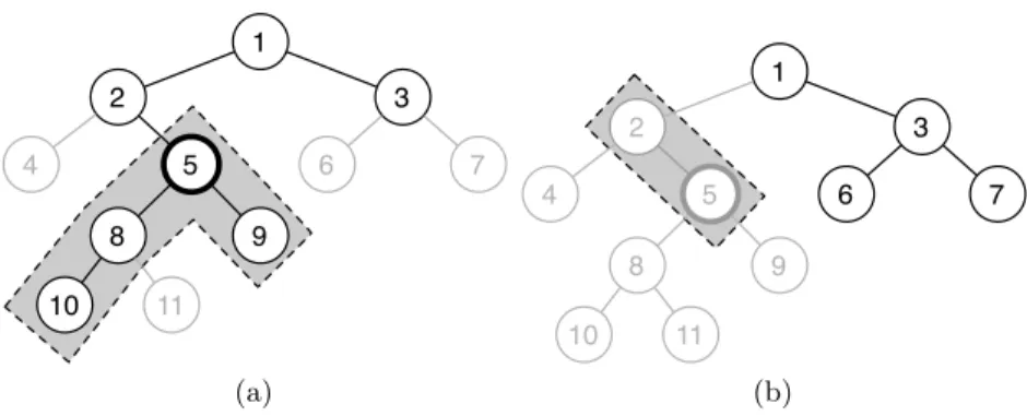
The graphs of Figure 1 illustrate with an example the assignment of costs detailed above.
3.3 Balanced learning
In the optimization problem Eq. 8,P OSandN EGsets may be very unbalanced, for instance, when we are using the first decomposition strategy of section 3.1, or if the number of siblings and their descendants is high. Thus, to adjust the weight of false positives and false negatives, following [10] we set a new optimization problem min 1 2hwj,wji+C + X i:xi∈P OS si·ξij+C− X i:xi∈N EG si·ξij, (11) s.t. yijhwj,xii ≥1−ξij, ξij≥0, ∀i:xi∈P OS∪N EG
where, using Eq. 9 and Eq. 10,
C+= X i:xi∈N EG si, C−= X i:xi∈P OS si. (12)
1 4 3 8 9 7 5 6 2 10 11 1 4 3 8 9 7 5 6 2 10 11 (a) (b)
Fig. 1. If we are trying to learn a model for class 5 (w5), the cost of a positive
ex-ample (xi,yi) withyi={1,2,3,5,8,9,10}(see graph (a)) is the sum of penalties for making false negatives classes{5,8,9,10}. On the other hand, the cost of a negative (xi,{1,3,6,7}), see graph (b), is the sum penalization (false positives) due to{2,5}
The idea is to balance the potential total cost of false positives and false neg-atives. Then the ratio of the regularization parameters C+ and C− must be inverse to the ratio of class sizes, where thesizeof the examples is its cost.
Additionally, we investigated if the possible benefits of balancing (as stated in Eq. 12) were due to the presence of costs or they were a consequence of the balancing itself. Thus we will use, in the experiments reported in the next section, a version with all costssi= 1 for alli.
4
Experimental results
For testing the hierarchical SVMs presented in this paper, we have carried out some experiments in order to compare their performance with two state-of-the-art learners that use different approaches. The algorithms used were H-M3-l∆of Rousu et al. [4], and HRLS of Cesa-Bianchi et al. [3]; while the first one searches for a global optimum loss (in this case the loss functionl∆of Eq. 4), HRLS takes a local point of view and it incrementally learns a linear-threshold for each node of the hierarchy of classes.
The comparison was done with a couple of benchmark information retrieval (IR) datasets. Thus, in addition to the loss functionsl0/1 (Eq. 2),l∆ (Eq. 4), we employed the performance measures:precision,recall, andF1.
The implementation of H-M3-l∆was provided by the author, and the scores of HRLS were taken from [4], where it is reported that the algorithm was imple-mented according to published descriptions of its authors. The implementation of the versions of HSVM were done modifying slightly Joachims’SV Mperf [11]; this SVM implementation provided us with an excellent base due to its linear complexity. In all cases, when it was needed, we set the regularization parameter
We tested two types of HSVMs. On the first hand we compared each of the three options (detailed in section 3.1) to decompose hierarchical classifications into a series of binary classifications tasks. So we used the subscript a for the option that usesall entries of the training set in all cases;sstands for the option that distinguishes betweensiblings; and finallypmeans the third option, where only are considered examplespredicted to belong to parent classes. The second dimension of versions was the kind of weighting scheme used. Thus, we built versions without any weighting at all, or using only costs (c) (Eq. 8), or using costs balancing (cb) (Eq. 11); we finally tested a weighted scheme that uses balancing without costs, that is, with all costssi= 1 (b).
Additionally, in order to test the performance of HSVMs in the presence of an increasing percentage of examples with multipath, we built a collection of artificial datasets specially devised for that purpose.
4.1 Results on IR datasets
We used two well-known datasets in information retrieval2. The documents were represented asbag-of-words and the features were scaled with theirinverse doc-ument frequency, in fact with the variant TFIFD [12, 13].
From the first dataset, REUTERS Corpus Volume 1 (RCV1) [14], following [4], 7500 documents were collected and 5000 were separated for testing purposes. The ’CCAT’ family of categories (Corporate/Industrial news articles) was used as the label hierarchy. This hierarchy represents a tree with maximum depth 3 and with a total of 34 nodes. The tree is quite unbalanced: there are 18 nodes residing in depth 1, 14 nodes in depth 2 and one node in depth 3. In this dataset, approximately 8% of examples have multiple partial paths; that is, these exam-ples were classified into classes that are not in the same path from the root.
The WIPO-alpha was published by the World Intellectual Property Organi-zation [15], and it is the second dataset used in these experiments. We used D section of the hierarchy. This section contains 1730 documents, and 358 of them were separated as test set. There are 188 nodes in the tree organized as follows: 7 in depth 1, 20 in depth 2, and 160 in depth 3. In this dataset there are no examples classified into more than one path.
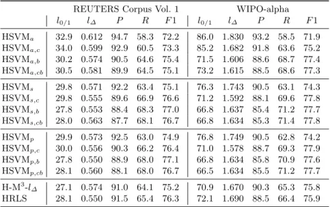
The left hand side of Table 1 depicts the scores obtained in RCV1 in the conditions described above. The key loss is l∆, since this is the optimization target; on the other hand, from an IR point of view F1 is the most relevant measure. In both measures HRLS outperforms H-M3-l∆. In the field of HSVM variants,sandpversions achieve better results than the one-vs-rest (a) variants; however, HSVMa,breaches the scores of H-M3-l∆inl∆and slightly better inF1. With respect to weighting schemes, balances (b) seem a bit better than costs (c), although with similar scores. In l∆ both HSVMsand HSVMpoutperform H-M3-l∆, even without any weighting; to reach the score of HRLS we need the balanced releases. InF1 any weighting outperform both HRLS and H-M3-l∆.
2
Table 1.Prediction losses l0/1,l∆, precision P, recall R and F1 on REUTERS and
WIPO datasets. All scores are given as percentages, but the values of the column labeled byl∆that are the average of Eq. 4 across the test set
REUTERS Corpus Vol. 1 WIPO-alpha
l0/1 l∆ P R F1 l0/1 l∆ P R F1 HSVMa 32.9 0.612 94.7 58.3 72.2 86.0 1.830 93.2 58.5 71.9 HSVMa,c 34.0 0.599 92.9 60.5 73.3 85.2 1.682 91.8 63.6 75.2 HSVMa,b 30.2 0.574 90.5 64.6 75.4 71.5 1.606 88.6 68.7 77.4 HSVMa,cb 30.5 0.581 89.9 64.5 75.1 73.2 1.615 88.5 68.6 77.3 HSVMs 29.8 0.571 92.2 63.4 75.1 76.3 1.743 90.5 63.1 74.3 HSVMs,c 29.8 0.555 89.6 66.9 76.6 71.2 1.592 88.1 69.6 77.8 HSVMs,b 27.8 0.553 88.4 68.3 77.0 66.8 1.637 85.4 71.2 77.7 HSVMs,cb 28.0 0.563 87.7 68.1 76.7 66.8 1.634 85.3 71.4 77.8 HSVMp 29.9 0.573 92.5 63.0 74.9 76.8 1.749 90.5 62.8 74.2 HSVMp,c 30.0 0.556 90.3 66.2 76.4 71.0 1.578 88.7 69.3 77.9 HSVMp,b 27.8 0.550 88.9 68.0 77.1 66.8 1.634 85.8 70.9 77.6 HSVMp,cb 28.1 0.560 88.1 68.0 76.7 66.5 1.634 85.5 71.2 77.7 H-M3-l∆ 27.1 0.574 91.0 64.1 75.2 70.9 1.670 90.3 65.3 75.8 HRLS 28.1 0.550 91.5 65.4 76.3 72.1 1.690 88.5 66.4 75.9
The scores in WIPO-alpha dataset are shown in the right hand side of Table 1. We can see bigger differences in this dataset than in RCV1. Again, versions of HSVM that use costs and/or balances attain better scores than those without any weighting, and better than H-M3-l∆and HRLS . In contrast with RCV1 results, in this case, the best result is found in HSVMp,c, not in HSVMp,b.
In general we see that the scores of HSVMsand HSVMpare quite similar, although the later seems that is able to slightly correct some mistakes of HSVMs. The strategy one-vs-rest (a) usually performs worse thansandp. With respect to weighting schemes, they reveal very useful both in costs or balances.
4.2 Artificial datasets
In order to test the ability of our approach to handle multiple paths, we devised an artificial dataset following a tree hierarchy. The tree has 44 nodes organized as follows: 3 in depth 1, 7 in depth 2, 9 in depth 3, 12 in depth 4, and 12 in depth 5. There are leaves at any depth, but in depth 0 and 1. All non-leaf-nodes have 2 or 3 children. We intended to simulate, in the artificial examples, a representation of the typebag-of-words. Therefore, we associated a numberρj of features to each nodej; and the values in features were generated following a uniform distribution between−1 and +1, but negative values were eliminated to achieve a sparse dataset. Examples were assigned to a node when the sum of the features attached to it exceed a given thresholdµj. We force the positive
0 5 10 15 0 0.02 0.04 0.06 0.08 0.1 0.12 0.14 0.16
% of multiple partial paths l∆ 0 5 10 15 95 96 97 98 99 100
% of multiple partial paths
F
1
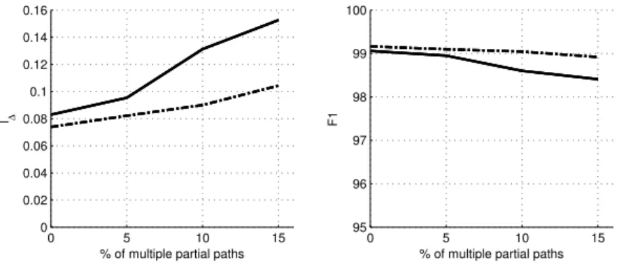
Fig. 2.Performance of the HSVMa,cb(solid line) and HSVMs,cb(dash-dot line) when the percentage of multiple partial paths in examples is increased. HSVMp,cband HSVMs,cbachieved exactly the same results
attribute values in order to ensure that we have 40 examples per node for training set and 20 per node for test set. We created artificial datasets with 0, 5, 10 and 15 pecentage of examples with multiple partial paths3. The parameters used in the experiment were:ρj= 50 andµj =ρj/0.7 for all j.
Figure 2 shows the performance of HSVMa,cb, HSVMs,cb, and HSVMp,cb, when the percentage of multiple partial paths is increased. HSVMs,cb, and HSVMp,cbreached exactly the same scores, and as it could be expected, they had better performance than HSVMa,cb. It is important to notice that HSVMs,cb(and HSVMp,cb) increased its l∆ in only 0.0305 classes failed per example, while the percentage of multiple partial paths had been increased from 0% to 15%. HSVMa,cbhad also a good performance, since its l∆ only was incremented in 0.0697. On the other hand, the behavior inF1 was quite parallel: HSVMs,cband HSVMp,cboutperform HSVMa,cb, but all had good resistance to the increase in the percentage of multipaths.
5
Conclusions
We have presented a learning method for hierarchical classifications tasks based on the use of learninglocalbinary classifications: one for each node of the hierar-chy. This approach is well known and it is acknowledged to achieve competitive results with other approaches [1, 3]. In the experiments reported in section 4, we also confirm the good scores of thisna¨ıveapproach. The novelty of this paper is the use for hierarchical classification of weighting schemas in binary classifiers.
We have studied two aspects: the decomposition of hierarchical tasks into binary classifications, and the definitions of weights suggested by both the hi-erarchy and the loss function. The conclusion is that it is possible to obtain a
3
A Matlab function for generating artificial datasets in this way can be downloaded from (http://www.aic.uniovi.es/MLGroup/DataSets/GenerateArtificial.m)
very competitive learning method, comparable with state-of-the-art algorithms [3, 4].
Additionally, in general the decomposition strategies have the advantage of modularity. So, it is possible to have fast parallel implementations for hierarchical classifications. Besides, each binary classification could be learned using well-known SVM implementations, and one could tune the regularization parameters or the kernels employed. Notice that if the application field is different from textual information, the choice of the right kernel may be a crucial point in the performance of any classification task.
Acknowledgments The research reported in this paper has been supported in part under Spanish Ministerio de Educaci´on y Ciencia (MEC) grant TIN2008-06247. The authors would like to thank Juho Rousu for the source code of his algorithm and Thorsten Joachims for the source code of SVMlightandSV MP erf.
References
[1] Dumais, S.T., Chen, H.: Hierarchical classification of web content. In: Proceedings of the 23rd SIGIR, NY, USA, ACM Press (2000) 256–263
[2] Cai, L., Hofmann, T.: Hierarchical document categorization with support vector machines. In: Proceedings of the 13thCIKM, NY, USA, ACM Press (2004) 78–87 [3] Cesa-Bianchi, N., Gentile, C., Zaniboni, L.: Incremental algorithms for
hierarchi-cal classification. JMLR7(2006) 31–54
[4] Rousu, J., Saunders, C., Szedmak, S., Shawe-Taylor, J.: Kernel-based learning of hierarchical multilabel classification models. JMLR7(2006) 1601–1626
[5] Cai, L., Hofmann, T.: Exploiting known taxonomies in learning overlapping con-cepts. In: Proceedings of the 20thIJCAI. (2007) 708–713
[6] Dekel, O., Keshet, J., Singer, Y.: Large margin hierarchical classification. In: Proceedings of the 21stICML. (2004) 209–216
[7] Dekel, O., Keshet, J., Singer, Y.: An efficient online algorithm for hierarchical phoneme classification. In: Proceedings of 1stInternational Workshop on Machine Learning for Multimodal Interaction. (2005) 146–158
[8] Hsu, C.W., Lin, C.J.: A comparison of methods for multiclass support vector machines. IEEE Transactions on Neural Networks13(2) (2002) 415–425 [9] Fan, H., Ramamohanarao, K.: A weighting scheme based on emerging patterns
for weighted support vector machines. In: Proceedings of IEEE International Conference on Granular Computing. (2005) 435– 440
[10] Morik, K., Brockhausen, P., Joachims, T.: Combining statistical learning with a knowledge-based approach - a case study in intensive care monitoring. In: Proceedings of the ICML. (1999) 268–277
[11] Joachims, T.: Training linear svms in linear time. In: Proceedings of the 12th SIGKDD, NY, USA, ACM Press (2006) 217–226
[12] Joachims, T.: Text categorization with support vector machines: learning with many relevant features. In: Proceedings of 10th ECML, (1998) 137–142
[13] Salton, G., Buckley, C.: Term weighting approaches in automatic text retrieval. Information Processing and Management24(5) (1988) 513–523
[14] Lewis, D.D., Yang, Y., Rose, T.G., Li, F.: Rcv1: A new benchmark collection for text categorization research. JMLR5(2004) 361–397