Optimization via Benders' Decomposition

Optimization via Benders’ Decomposition

by

Hiruni Kamali Pallage

B.Sc., University of Sri Jayewardenepura, 2014

Submitted to the Graduate Faculty of

the Kenneth P. Dietrich School of Arts and Sciences in partial

fulfillment

of the requirements for the degree of

Master of Science

University of Pittsburgh

2019

UNIVERSITY OF PITTSBURGH

KENNETH P. DIETRICH SCHOOL OF ARTS AND SCIENCES

This thesis was presented by

Hiruni Kamali Pallage

It was defended on July 12, 2019 and approved by

Jeffrey Paul Wheeler, Ph.D., Lecturer II, Mathematics, University of Pittsburgh Michael A. Trick, Harry B. and James H. Higgins Professor of Operations Research; Dean,

Carnegie Mellon University Qatar

G. Bard Ermentrout, Distinguished University Professor, Mathematics, University of Pittsburgh

Jason DeBlois, Associate Professor, Mathematics, University of Pittsburgh Michael Schneier, Post-Doctoral Associate, Mathematics, University of Pittsburgh Thesis Advisor: Jeffrey Paul Wheeler, Ph.D., Lecturer II, Mathematics, University of

Optimization via Benders’ Decomposition

Hiruni Kamali Pallage, M.S. University of Pittsburgh, 2019

In a period when optimization has entered almost every facet of our lives, this thesis is designed to establish an understanding about the rather contemporary optimization tech-nique: Benders’ Decomposition. It can be roughly stated as a method that handles problems with complicating variables, which when temporarily fixed, yield a problem much easier to solve. We examine the classical Benders’ Decomposition algorithm in greater depth followed by a mathematical defense to verify the correctness, state how the convergence of the algo-rithm depends on the formulation of the problem, identify its correlation to other well-known decomposition methods for Linear Programming problems, and discuss some real-world ex-amples. We introduce present extensions of the method that allow its application to a wider range of problems. We also present a classification of acceleration strategies which is cen-tered round the key sections of the algorithm. We conclude by illustrating the shortcomings, trends, and potential research directions.

Table of Contents

Preface . . . ix

1.0 Introduction . . . 1

2.0 History . . . 3

3.0 Definitions and Examples . . . 4

3.1 Primal and Dual Linear Programs . . . 5

3.2 Basic Model of Benders’ Decomposition . . . 9

3.3 Solution Steps for the Algorithm . . . 10

3.4 Alternative Form of Benders Cuts . . . 15

3.5 The Algorithm with a Relaxed Master Problem . . . 18

4.0 The Algorithm and its Justification . . . 24

5.0 Extensions and Generalizations of Benders’ Decomposition Algorithm 34 5.1 Generalized Benders’ Decomposition . . . 35

5.2 Logic-based Benders’ Decomposition . . . 36

5.3 Combinatorial Benders’ Decomposition . . . 37

5.4 L-shaped Decomposition . . . 37

5.5 Nested Benders’ Decomposition . . . 38

6.0 Applications . . . 39

6.1 The Facility Location Problem . . . 39

6.1.1 General Problem [6] . . . 40

6.1.2 An Actual Example [6] . . . 42

6.2 The Intensity Modulated Radiation Therapy Problem . . . 48

6.2.1 General Problem [33] . . . 48

6.2.2 An Actual Example [33] . . . 52

6.3 Advanced Applications . . . 56

6.3.1 Simultaneous Aircraft Routing and Crew Scheduling . . . 57

6.3.3 The Concrete Delivery Problem . . . 58

6.3.4 The Lock Scheduling Problem . . . 58

7.0 Conclusion . . . 59

7.1 Model Selection for Benders’ Decomposition . . . 59

7.2 Relationship to Other Decomposition Methods . . . 59

7.3 Shortcomings of Benders’ Decomposition . . . 60

7.4 Enhancement Strategies of Benders’ Decomposition . . . 60

7.5 Promising Research Directions . . . 62

7.6 Commercial Software that Implements Benders’ Decomposition . . . 63

Appendix A. Linear Programming. . . 65

A.1 Preliminaries . . . 65

A.2 Graphical Method . . . 67

A.3 Simplex Method . . . 71

A.3.1 Artificial Variables Technique . . . 74

Appendix B. Integer Programming . . . 78

B.1 Preliminaries . . . 78

B.2 Cutting Plane Algorithm . . . 78

B.3 Branch and Bound Algorithm . . . 84

Bibliography . . . 88

List of Tables

1 Some applications of Benders’ Decomposition algorithm from [27] . . . 2

2 Some optimization problems solved via Benders’ Decomposition from [27] . . 3

3 The relationship between solutions of primal and dual problems . . . 7

4 The relationship between primal and dual problems from [30] . . . 8

5 Some versions of Benders’ Decomposition algorithm . . . 35

6 Basic data corresponding to Example 6.1.2 from [6] . . . 42

7 Classification of enhancement strategies from [27] . . . 60

A.1 Initial Simplex table . . . 72

A.2 Basic data corresponding to Example A.3 . . . 75

A.3 Initial Simplex table corresponding to Example A.3 . . . 76

A.4 Calculations leading to the second Simplex table corresponding to Example A.3 76 A.5 Second Simplex table corresponding to Example A.3 . . . 77

A.6 Final optimal Simplex table corresponding to Example A.3 . . . 77

B.1 Initial Simplex table corresponding to Example B.1 . . . 81

B.2 Final optimal Simplex table corresponding to Example B.1 . . . 81

B.3 New initial Simplex table corresponding to Example B.1 . . . 83

B.4 New final optimal Simplex table corresponding to Example B.1 . . . 83

List of Figures

1 Schematic representation of Benders’ Decomposition algorithm from [27] . . . 5

2 Flowchart of classical Benders’ Decomposition algorithm from [30] . . . 12

A.1 Feasible region corresponding to Example A.1 . . . 69

A.2 Feasible region corresponding to Example A.2 . . . 70

B.1 Gomory cuts . . . 79

B.2 Initial feasible region corresponding to Example B.1 . . . 80

B.3 New feasible region corresponding to Example B.1 . . . 82

B.4 Branch and Bound algorithm . . . 84

List of Algorithms

1 Classical Benders’ Decomposition Algorithm from [30] . . . 10

2 The Classical Algorithm with a Relaxed Master Problem from [33] . . . 20

3 Multi Step Procedure for Solving Problems of the Form (4.1) from [1] . . . . 30

A.1 Linear Programming Problem Formulation . . . 66

A.2 Graphical Method . . . 67

A.3 Simplex Method . . . 73

A.4 The Big M-method . . . 74

B.1 Cutting Plane Algorithm . . . 79

Preface

It is a pleasure to pay tribute to one and all who provided me unflinching encouragement and support in various ways to complete my research work.

First and foremost, I wholeheartedly appreciate my wonderful advisor, Dr. Jeffrey Wheeler, for his patience, motivation, enthusiasm, and immense knowledge. I have spent many hours in productive and fruitful conversation on research and life with my outstanding advisor. Thank you for going above and beyond the role of an advisor and being that person who understood the challenges that graduate school brought into everyday life.

Besides my advisor, I would like to thank Professor Michael A. Trick (Carnegie Mel-lon University, Qatar) for his intellectual contributions to the work. It was a wonderful experience to work with such an intelligent expert in Operational Research field.

I would also like to thank the rest of my thesis committee: Professor G. Bard Ermentrout (University of Pittsburgh), Professor Jason DeBlois (University of Pittsburgh), and Dr. Michael Schneier (University of Pittsburgh) for their encouragement, valuable time and insightful comments.

Moreover, I owe a great deal to the Department of Mathematics and the University of Pittsburgh for providing me such a great place to broaden my mathematical sphere of knowledge, and to meet so many great and nice friends of my life. I also want to thank all my friends for their help and encouragement in my graduate study and in my life.

Thank you, Mom and Dad for the emotional support, intellectual stimulation and many hours of identity-forming conversation, inspiring me to pursue unconventional dreams in which I truly believe. You are the most supportive parents one could hope for.

Last but not the least, I record my unstinted thanks to my loving and tolerant husband Achna for his faithful support rendered throughout, comforting me in the hardest times.

1.0 Introduction

The objective of any company is to maximize its profits and efficiently use its resources. In attempting to complete a project without a schedule, for example, one may accomplish the goals but not without wasted time and money. As a result, optimization and scheduling has become a tremendous problem for the management of companies and recent years have seen an increased demand for the application of mathematics to develop the perfect schedule to meet the goals.

“Optimization via Benders’ Decomposition” (BD) addresses the perennial problem of optimal utilization of finite resources in the accomplishment of an assortment of tasks or objectives. The thesis refers to applications which provide ways to uncover the core of the above real-world challenges, present them in mathematical terms, and devise mathematical solutions for them with the use of BD algorithm.

The main focus of the BD algorithm is to deal with problems where certain variables are temporally fixed yielding a problem considerably easier to solve. The BD method has now developed to be one of the most extensively used exact algorithms since it utilizes the structure of the problem to decentralize the total computational weight. Successful applications are found in many diverse fields, including planning and scheduling.

The remainder of the thesis is organized as follows. After discussing the history related to the BD algorithm, Chapter 3 presents the theory behind the classical BD algorithm followed by simple examples where Chapter 4 offers a mathematical justification to prove the correctness of the algorithm. Then, Chapter 5 focuses on the extensions and generalizations of BD algorithm leading to Chapter 6; which will be about some of the applications of the algorithm where applications are selected from several fields to show the reach of the BD algorithm. Finally, Chapter 7 provides concluding remarks and describes other promising research directions of the algorithm. Further, a primer on Linear Programming and Integer Programming is offered in the Appendix.

We conclude the introduction by illustrating the evolution of the BD algorithm in various fields, giving an informative table provided in The Benders’ Decomposition Algorithm: A

Literature Review, [27].

Reference Application Reference Application

1 Behnamian (2014) Production planning 17 Jiang et al. (2009) Distribution planning 2 Adulyasak et al. (2015) Production routing 18 Kim et al. (2015) Inventory control 3 Boland at al. (2015) Facility location 19 Laporte et al. (1994) Traveling salesman 4 Boschetti & Maniezzo (2009) Project scheduling 20 Luong (2015) Healthcare planning 5 Botton al. (2013) Survivable network design 21 Maravelias & Grossmann (2004) Chemical process design 6 Cai et al. (2001) Water resource management 22 Moreno-Centeno and Karp (2013) Implicit hitting sets 7 Canto (2008) Maintenance scheduling 23 Oliveira et al. (2014) Investment planning 8 Codato & Fischetti (2006) Map labeling 24 Osman and Baki (2014) Transfer line balancing 9 Cordeau et al. (2006) Logistics network design 25 P´erez- Galarce et al. (2014) Spanning tree

10 Cordeau al. (2001a) Loocomotive assignment 26 Pishvaee et al. (2014) Supply chain network design 11 Cordeau et al. (2001b) Airline scheduling 27 Rubiales et al. (2013) Hydrothermal coordination 12 Corr´ea et al. (2007) Vehicle routing 28 Saharidis et al. (2011) Refinery system network planning 13 Cˆot´e et al. (2014) Strip packing 29 Sen et al. (2015) Segment allocation

14 Fortz and Poss (2009) Network design 30 Bloom (1983) 13 Capacity expansion 15 Gelareh et al. (2015) Transportation 31 Wang et al. (2016) Optimal power flow 16 Jenabi et. Al. (2015) Power management

2.0 History

Jacobus Franciscus (Jacques) Benders (1924 - 2017) was the first professor in the Nether-lands in the field of Operations Research and is known for his role in mathematical program-ming [37]. He obtained his PhD in 1960 with the thesis titled “Partitioning in Mathematical Programming” from Utrecht University. Starting his career as a statistician for the Rubber Foundation in late 1940s, he then moved to Shell Laboratory in Amsterdam in 1955. He researched mathematical programming problems regarding the logistics of the oil refinery and developed the method name after him. Benders was designated Professor of Operations Research at the Eindhoven University of Technology in 1963 and retired in 1989. Further-more, in 2009, he was bestowed the EURO Gold Medal, the highest distinction in the area of Operations Research in Europe. Although the algorithm was first introduced to solve the Mixed-Integer Linear Programming (MILP) problems, later developments were made to apply the algorithm to a broader range of problems and to increase its efficiency on certain optimization classes.

Reference Model Reference Model

1 Adulyasak et al. (2015) Multi-period stochastic problem 11 Jenabi et al. (2015) Piecewise linear mixed-integer problem 2 Behnamian (2014) Multi-objective MILP 12 Kim et al. (2015) Multi-stage stochastic program 3 Cai et al. (2001) Multi-objective nonconvex nonlinear problem 13 Laporte et al. (1994) Probabilistic integer formulation 4 Cordeau et al. (2001b) Pure 0−1 formulation 14 Li (2013) Large-scale nonconvex MINLP

5 Corr´ea et al. (2007) Binary problem with logical expressions 15 Moreno- Centeno & Karp (2013) Problem with constraints unknown in advance 6 Gabrel et al. (1999) Step increasing cost 16 Bloom (1983) Nonlinear multi-period problem with reliability constraint 7 Cˆot´e et al (2014) MILP with logical constraints 17 Osman and Baki (2014) Nonlinear integer formulation

8 de Camargo et al (2011) Mixed-integer nonlinear program (MINLP) 18 P´erez-Galarce et al. (2014) Minmax regret problem

9 Emami et al. (2016) Robust optimization problem 19 Pishvaee et al. (2014) Multi-objective possibilistic programming model 10 Fontaine & Minner (2014) Bilevel problem with bilinear constraints 20 Raidl et al. (2014) Integer, bilevel, capacitated problem

3.0 Definitions and Examples

We begin by highlighting the significance of Benders’ Decomposition (BD) algorithm as an approach for solving certain large-scale optimization problems. When it comes to con-structing and solving optimization problems a major concern is that the amount of memory and the computational effort required to solve such problems will grow substantially with the number of variables and constraints. The conventional method of making all decisions simultaneously by solving a massive optimization problem quickly turns out to be intractable with the increase in the number of variables and constraints. To alleviate this difficulty, mul-tistage optimization algorithms such as BD have been developed as an alternative solution methodology. Unlike the traditional methods, these algorithms split the decision-making process into several phases.

In reality, the first step of the BD algorithm is to fix certain variables in the original problem, thus making the resulting subproblem easy to solve. Throughout the thesis we refer to those variables, which make the problem significantly easier to solve when fixed, as complicating variables. So it is clear that the core of BD algorithm is to identify the right decomposition for the given model (that is, the right partitioning of the variables). This decision usually demands specific knowledge of the problem at hand including known methods to solve similar problems quickly. It is hence not possible for us within the scope of this thesis to give a complete outline of BD algorithm that works for all problems. However, in Section 3 and 6 we provide some concrete examples where we choose certain variables to be fixed and employ BD algorithm successfully to solve the problem.

In BD, the problem is divided into a master problem (MP) and a subproblem (SP), which are then solved iteratively. The MP which considers a subset of the variables, is solved first. Next, we temporarily fix the variables’ values of the MP and solve the SP for the remaining variables. Finally, depending on the solution of the SP, one or more cuts are derived and added to the MP, thus effectively averting the MP from returning to similar areas of the search space. Note that in the classical Benders’ Decomposition the SP is a Linear Programming problem, where cuts are generated based on the outcome of its dual

problem (DSP). Benders’ Decomposition (BD) Master Problem (MP) Dual Subproblem (DSP) Feedback (cuts) Information (solutions) 0 i

Figure 1: Schematic representation of Benders’ Decomposition algorithm from [27]

Regarding cuts, we note that current Integer Programming techniques walk us around corner points of the feasible region in search of corner points that lead to feasible solutions. If it does not arrive at a feasible solution at a specific corner point, the main approach is to cut away that part of the feasible region by introducing a new constraint which throws out that corner point. At the same time, it ensures not to throw off the corner point/s where the optimal value occurs. So, in generalcutsare additional constraints that cut the feasible region to reduce the solution search space to simply contain feasible solutions.

3.1 Primal and Dual Linear Programs

As mentioned in the previous section, we need to understand concepts of duality in linear programs before we dive into the basic model and solution steps of BD algorithm. We consider a Linear Programming (LP) problem that can be expressed in matrix notation as follows:

M aximize P =cTx such that Ax_≤b

where c, x _{∈ R}n, b _{∈ R}m and A _{∈ R}m×n_{. The linear function c}T_{x is the objective} function and the linear inequalities are the constraintswhich generate afeasible region to minimize the objective function. The solutions of the primal problem in the feasible region can be written as _{x_∈Rn_|Ax_≤b,x_≥0_}.

We refer to the above original LP as the primal problem and any primal problem can be expressed in another LP form which is called the dual problem. The corresponding dual problem to the above primal problem can be expressed as follows:

M inimize C=bTy such that ATy_≥c

y_≥0.

These two forms are linked by the following theorem:

Theorem 1 (The Fundamental Principle of Duality from [36]).

A minimization problem has a solution if and only if the corresponding dual maximization problem has a solution.

In more specific terms: Theorem 2 (from [36]).

If x satisfies the constraints of a Linear Programming problem in primal form and if y

satisfies the constraints of the corresponding dual, then cTx_≤bTy.

Proof. From the primal form, we have that x _≥ 0 and Ax _≤ b. Similarly, by the dual

y_≥0 and AT_{y ≥c are satisfied. Hence}

cTx_≤(ATy)Tx=yTAx_≤yTb=bTy

We know that every LP is either feasible or not feasible and that feasible problems either are unbounded or have a solution. We say that an LP has a feasible solution if there exists a set of values for the decision variables that satisfies all the constraints. When it is impossible to find a feasible solution, that is, when we cannot obtain a solution that meets each constraint, LP is said to be infeasible. An unbounded solution to an LP with the objective of maximizing (minimizing) is when it is possible to construct the solution to be infinitely large (small) while none of the constraints are violated. From the above theorem we can conclude that if primal is unbounded, then dual is infeasible. Likewise, if dual is unbounded, then primal is infeasible. The Duality Theorem allows us to understand more possible relationships among solutions of primal and dual.

Theorem 3 (Duality Theorem for Linear Programs).

For a primal-dual pair of Linear Programming problems, one of these four cases occurs: 1. Both are infeasible.

2. Primal is unbounded and dual is infeasible. 3. Dual is unbounded and primal is infeasible.

4. Both are feasible and there exist optimal solutions x, y to primal and dual such that

bTy=cTx.

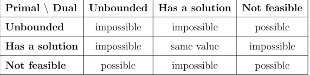
Another way to think about this relationship is to create a table of possibilities. We take each of the three rows to denote one of three possibilities of the primal solution. The columns denote the same characteristics of the dual solution. An alternative method to justify the table below is to examine the Simplex Method which solves primal and dual simultaneously.

Primal _\ Dual Unbounded Has a solution Not feasible Unbounded impossible impossible possible Has a solution impossible same value impossible Not feasible possible impossible possible

Any discussion on the duality of LP problems will be incomplete without understanding how to convert a given primal LP to its corresponding dual. Assuming that the primal has M constraints andN variables, now we summarize the relationship between primal and dual:

Primal (or dual) Dual (or Primal)

Objective Maximize P Minimize C Objective

Variable (N) ≥0 ≥ Constraints (N) ≤0 _≤ unbounded = Constraints (M) ≤ ≥0 Variable (M) ≥ ≤0 = unbounded

Right side of constraints Coefficients of variables in objective functions Coefficients of variables in objective functions Right side of constraints

Table 4: The relationship between primal and dual problems from [30]

Now we consider an easy example to find the dual of the given primal problem. Primal Problem M aximize P = 15x1+ 14x2+ 16x3 such that x1+ 2x2 ≥21 x1+x3 ≤31 −5x1+ 8x2+x3 ≤ −51 x1−x2+x3 = 11 x1 ≥0, x2 ≤0, x3 unbounded Dual Problem M inimize C = 21y1+ 31y2−51y3+ 11y4 such that y1+y2−5y3 +y4 ≥15 2y1+ 8y3−y4 ≤14 y2+y3+y4 = 16 y1 ≤0, y2, y3 ≥0, y4 unbounded

The number of inequalities (variables) in the primal becomes the number of variables (inequalities) in the dual. Thus, the dual may differ in the dimension from the primal and it may be desirable to solve an LP with fewer constraints.

3.2 Basic Model of Benders’ Decomposition

We now carry on to describe the basic model of BD algorithm which is critical for understanding all the proceeding discussions in the thesis. Here we consider a Mixed Integer Linear Program (MILP), that is, the original problem (P1) of the following general form:

M inimize z =cTx+fTy such that Ay_≥b

Bx+Cy_≥d x_≥0, y_∈Y⊆Zn

with complicating variables y _∈Zn which must fit the constraint Ay_≥b, whereA_∈Rm×n is a known matrix andb_∈Rm is a given vector. The variablesx_∈Rs, as well asyvariables, should satisfy the connecting constraint Bx+Cy _≥ d, where B _∈ Rr×s, C ∈ Rr×n, and

d_{∈ R}r. The objective function is to minimize the total cost together with the cost vectors

f _∈Zn andc_∈Rs. Note that, xhaving real components andyhaving integer components, make the above a MILP.

We suppose that the y variables are complicating variables, so if y variables are fixed, the problem is linear inxand becomes significantly easier to solve. Hence, P1 can be stated as: min

y∈R

fTy_|Ay _≥b+ min_{Bx_≥d₋Cy,x_≥0_} with R = _{y_| there exist x _≥ 0 such that Bx _≥ d₋Cy,x _≥ 0, Ay _≥ b, y _{∈ Y}}. So P1 can be divided into an MP that contains the y variables and an SP that contains the x variables.

Master Problem (MP) M inimize zlower

such that zlower ≥fTy

Ay_≥b y _∈Y Primal Subproblem (SP) M inimize cTx such that Bx_≥d₋Cyˆ x_≥0

Also note that taking u to be the dual variable associated withBx_≥d₋Cyˆ, the dual subproblem (DSP) of SP can be written as:

M aximize (d₋Cyˆ)T_u such that BT_u≤c

u _≥0.

3.3 Solution Steps for the Algorithm

Here we present a basic idea behind the algorithm before formally stating it. After developing the initial MP and SP, the algorithm starts with the MP and alternates between MP and SP till an optimal solution is derived. The objective function of the MP generates a fitting lower bound on the optimal cost; while combining the ˆysolution with the objective value of the SP (which is equivalent to fixing ˆy in the original problem) provides a valid upper bound on the optimal cost. Then, the optimality gap is computed in each iteration to confirm the convergence of the algorithm. The classical BD approach uses the Branch and Bound algorithm to solve the MP and the Simplex Method is employed to tackle the SP. We will now move our attention to describing BD algorithm in greater depth using mathematical terms.

Algorithm 1 Classical Benders’ Decomposition Algorithm from [30] 1. Initialize ˆy and set as necessary.

2. Solve MP1 and find an initial lower bound solution ˆzlower at ˆy.

• If MP1 is infeasible so is the original problem P1.

• If MP1 is unbounded, set ˆzlower = ∞ in MP1 for an arbitrary value of ˆy in Y, and proceed to step 3.

3. Solve SP or DSP to get an upper bound solution to the original problem P1.

Solving DSP: ˆzupper = fTyˆ+ (d−Cyˆ)Tuˆ is the upper bound solution for optimal dual solution ˆu. Solving SP: ˆzupper =cTxˆ+fTyˆ is the upper bound solution for the original problem P1 for ˆx.

• If |zˆlower − zˆupper| ≤ for P1, the process is terminated. Otherwise, add a new constraint (feasibility cut) zlower ≥ fTy+ (d−Cy)Tuˆ to MP1 to form MP2 and proceed to step 4.

• If DSP is unbounded (that is, SP is infeasible), then introduce a new cut (infeasibility cut) (d₋Cy)T_{uˆ ≤0 to MP1 to form MP2. Now we use a new SP, feasibility check} subproblem below to calculate u in DSP to form the infeasibility cut and then proceed to step 4.

M inimize 1Ts

such that Bx+1s_≥d₋Cyˆ _→uˆ

x_≥0, s_≥0

• If DSP is infeasible (that is SP is unbounded or infeasible), the original problem P1 will have either no feasible solution or an unbounded solution. So the process terminates.

4. Solve the updated master problem MP2 to find a new lower bound solution ˆzlower for the original problem P1, with respect to ˆy. In the following MP2 formulation, either the feasibility cut (second constraint) or the infeasibility cut (third constraint) can be used as discussed in Step 3. M inimize zlower such that Ay_≥b zlower ≥fTy+ (d−Cy)Tuˆ (d₋Cy)Tuˆ _≤0 y _∈Y

Then return to step 3 to solve the subproblem SP or the dual of the subproblem DSP again. If MP2 is unbounded, specify ˆzlower =∞and return to step 3. If MP2 is infeasible, so is the original problem P1. So, the process terminates.

Note that it is common in literature to refer the feasibility cut as theoptimality cut and the infeasibility cut as the feasibility cut.

Having used the previous pages to explain how classical BD works, we will now provide a flowchart that summarizes the above discussion.

Start

Initialize ˆy

set

Solve the Initial Master problem (MP1) for ˆzlowerat ˆy

(if MP1 has an unbounded solution, set ˆzlower = ∞) Infeasible solution to MP Infeasible solution toP1 Stop

Solve the new master prob-lem (MP2) with more constraints for ˆzlowerat ˆy. Solve the subproblem (SP) for ˆxor solve the dual of the subproblem (DSP) for ˆu, at ˆy. DSP has a solution (SP has a solution) Update ˆ zupper= fTyˆ+ (d−Cyˆ)T_uˆ (ˆzupper = fT_ˆy +cT_xˆ)

Check|zlowerˆ −ˆzupper| ≤

Converged Optimal

Solution

Add a new Benders’ cut (feasiblity cut) to MP1 to generate MP2 ˆ zlower ≥fT_{y+ (d} −Cy)T_uˆ DSP infeasible (SP infeasible or unbounded) Infeasible or Unbounded Solution to P1 Stop DSP unbounded (SP infeasible)

Add a new Benders’ cut (infeasiblity cut) to

MP1 to generate MP2 (d−Cy)T_{uˆ ≤ 0}

Y

N

1

Figure 2: Flowchart of classical Benders’ Decomposition algorithm from [30]

We revisit the general idea behind the algorithm to explain some key facts that the careful reader may have already observed.

Given the original problem (P1) our goal is to find values of variables x, y, and the objective functionz. We solve the MP to get a lower bound solution toz (that iszlower) and solve the primal/dual SP to get an upper bound solution to z (that is zupper). We continue the process until the values of z are within the tolerance. In other words, MP and the SP work together to generate a solution to P1.

zlowerin the MP is in fact a relaxation ofz in P1. Since we do not have value ofxvariable at the beginning of the process we relax thex variable inz and employ BD algorithm which finds appropriatexvalues and represent them as ideally a small number of constraints which we then introduce to the MP. That is, even though the variable xdoes not appear explicitly in the MP, it is represented by the various constraints (feasibility and infeasibility cuts) that are generated by the SP. These cuts are implicitly representing effect of x in P1. So once we generate all the constraints related to each feasiblex in the primal SP then thezlower in the MP will equal to the z in P1. Thus, MP is implicitly the same problem as P1.

Here we explain what motivates the choice of feasibility and infeasibility cuts to be defined as we stated in step 3 of Algorithm 1. Suppose we figure out a feasible ˆu for the DSP for which the DSP is unbounded. It means that this ˆuis a direction of unboundedness for which the objective function value of the DSP (d₋Cyˆ)T_{u>0. So as long as we choose} any ˆy for which (d₋Cyˆ)T_{uˆ >0 then the DSP will be made unbounded. Thus in order to} avoid this unbounded ray we got to choose a ˆy that does not allow (d₋Cyˆ)T_{uˆ > 0. In} other words, we must introduce (d₋Cy)T_{uˆ ≤ 0 (infeasibility cut) to the MP to restrict} the movement in this direction. Feasibility cut works really the same way because at this point we have a feasible ˆu which created a finite objective function value for the DSP (as well as a feasible ˆxwhich generated a finite objective function value for the SP). We update the upper bound solution to z using ˆzupper = fTyˆ+ (d−Cyˆ)Tuˆ or ˆzupper = cTxˆ +fTyˆ. Now if we are not within the tolerance, we introducezlower ≥fTy+ (d−Cy)Tuˆ (feasibility cut) which can be similarly expressed as zlower ≥ fTy+cTxˆ to the MP which says that if we need a better DSP/SP value we better avoid this solution.

In this chapter we give little attention to developing a complete discussion on LP even though we use concepts related to LP extensively. However, we provide more details in the Appendix which includes Linear Programming as well as Integer Programming.

To enhance the understanding of how the BD algorithm works, we now illustrate a simple numerical example.

Example 1.

Solve the following MILP, P1 [30] using the BD algorithm.

M inimize x+y such that 2x+y_≥3

x≥0, y ∈ {−5,−4,−3, ...,3,4}

Comparing with the basic model for BD: cT = [1], fT = [1], B = [2], C = [1], d= [3].

Iteration 1: Master Problem (MP1) M inimize zlower such that zlower ≥y y ∈ {−5,−4, ...,3,4} Primal Subproblem (SP) M inimize x such that 2x_≥3₋yˆ x≥0 Dual Subproblem (DSP) M aximize (3₋yˆ)u such that 2u_≤1 u≥0

The lower bound optimal solution to the original problem is: zˆlower =−5 when yˆ=−5.

Now we solve the DSP when yˆ=−5.

M aximize 8u such that 2u≤1

u_≥0

The optimal solution to DSP is 4 when u= 1/2. Thus, zˆupper = fTyˆ+ (d−Cyˆ)Tuˆ = ˆ

y+ 4 = ₋5 + 4 = ₋1. Since zˆupper = −1 > zˆlower = −5 we continue to the next iteration.

So, we need to introduce a new cut (feasibility cut), zlower ≥ fTy+ (d−Cy)Tuˆ to MP1 to

form MP2. The new Benders’ cut can be written as:

zlower ≥fTy+ (d−Cy)Tuˆ zlower ≥y+ (3−y) 1 2 zlower ≥ 3 2 + 1 2y.

Iteration 2:

The new master problem MP2:

M inimize zlower such that zlower ≥y

zlower ≥ 3₂ + 1₂y y_{∈ {−}5,₋4, ...,3,4_}.

The new lower bound optimal solution to the original problem is: zˆlower = −1 when

ˆ

y=−5. Then we solve the DSP when yˆ=−5.

M aximize 8u such that 2u≤1

u_≥0

The optimal solution to DSP is again 4 when u= 1/2. Thus,zˆupper =fTyˆ+ (d−Cyˆ)Tuˆ = ˆy+ 4 = ₋5 + 4 = ₋1. Now since zˆupper = −1 = ˆzlower the process has converged. The

solution for the SP (using the optimal solution to DSP) is x = 4. Thus, x= 4 and y =−5

minimizes the the original problem P1 and P1min =_{x+y_}min =−1.

3.4 Alternative Form of Benders Cuts

Here we switch focus to a slightly different form of representing the Benders’ cuts [30]. Recall that the Benders’ cuts that were introduced had the form:

zlower ≥fTy+ (d−Cy)Tuˆ f easibility cut (d₋Cy)Tuˆ _≤0 inf easibility cut

which can also be represented as:

zlower ≥fTy+w( ˆy)−(y−yˆ)TCTuˆ f easibility cut v( ˆy)−(y₋yˆ)TCTuˆ _≤0 inf easibility cut

where w( ˆy) is the optimal solution of SP and v( ˆy) is the optimal solution of the feasibility check subproblem. Herezlower ≥fTy+w( ˆy)−(y−yˆ)TCTuˆ shows that the objective value

of the original problem is decreased by updatingy from ˆyto a new value. ˆu_∈Rs indicates the incremental change in the optimal objective. v( ˆy)₋(y₋yˆ)T_CT_{uˆ ≤ 0 shows that ˆy} is updated to a new value to eliminate constraint violations in SP based on ˆy given in the master problem. ˆu_∈Rt indicates the incremental change in the total violation.

Example 2.

Solve the following MILP, P1 [30] using the alternative form of BD algorithm stated above.

M inimize x1 + 3x2+y1+ 4y2

such that ₋2x1− x2+ y1−2y2 ≥1

2x1+ 2x2−y1+ 3y2 ≥1

x1, x2 ≥0, y1, y2 ≥0 Comparing with the basic model for BD:

cT =h1 3 i , fT =h1 4 i , B =   −2 −1 2 2  , C =   1 −2 −1 3  , d=   1 1  . Iteration 1: Master Problem (MP1) M inimize zlower such that zlower ≥y1+ 4y2 y1 ≥0, y2 ≥0 Primal Subproblem (SP) M inimize x1+ 3x2 such that −2x1−x2 ≥1−yˆ1+ 2ˆy2 2x1+ 2x2 ≥1 + ˆy1−3ˆy2 x1, x2 ≥0

The lower bound optimal solution to the original problem is: zˆlower = 0 whenyˆ1 = ˆy2 = 0. Now we solve the SP when yˆ1 = ˆy2 = 0.

M inimize x1+ 3x2

such that −2x1−x2 ≥1

2x1+ 2x2 ≥1

Applying Simplex Method we can see that the solution to the SP is not feasible. Thus we need to introduce a new cut (infeasibility cut), v( ˆy)₋(y₋yˆ)T_CT_{uˆ ≤ 0 to MP1 to form}

MP2. The feasibility check subproblem below is used to calculateuˆ in DSP to form the above infeasibility cut. The feasibility check subproblem can be written as:

M inimize 1T_s such that Bx+1s_≥d₋Cyˆ _⇒ x_≥0, s_≥0 M inimize s1+s2 such that ₋2x1−x2+s1 ≥1−yˆ1+ 2ˆy2 2x1+ 2x2+s2 ≥1 + ˆy1−3ˆy2 x1, x2 ≥0, s1, s2 ≥0.

Applying the Simplex Method to the above feasibility check subproblem we can see that the optimal solution is 1.5 and values of the associated dual variables are uˆ1 = 1.0, uˆ2 = 0.5. Now for yˆ1 = ˆy2 = 0 the Benders’ cut can be written as:

v( ˆy)₋(y₋yˆ)TCTuˆ _≤0

1.5₋0.5(y1−yˆ1) + 0.5(y2 −yˆ2)≤0

y1−y2 ≥3. Iteration 2:

The new Master Problem MP2:

M inimize zlower

such that zlower ≥y1+ 4y2

y1−y2 ≥3

y1 ≥0, y2 ≥0.

The lower bound optimal solution of the original problem is: zˆlower = 3foryˆ1 = 3, yˆ2 = 0. We now solve the SP when yˆ1 = 3, yˆ2 = 0.

M inimize x1+ 3x2

such that −2x1−x2 ≥ −2

2x1+ 2x2 ≥4

x1, x2 ≥0

Now the primal subproblem SP is feasible with an optimal solution of 6 with primal variables being equal to xˆ1 = 0, xˆ2 = 2 and dual variables being equal to uˆ1 = 2.0, uˆ2 = 2.5

(values were read from optimal Simplex table for SP). Thus the upper bound solution of the original problem is: zˆupper =cTxˆ+fTyˆ= 6+ ˆy1+4ˆy2 = 6+3 = 9.Sincezˆupper = 9> zlower = 3 we continue to the next iteration. As well we need to introduce a new cut (feasibility cut),

zlower ≥ fTy+w( ˆy)−(y−yˆ)TCTu to MP2 to form MP3. For yˆ1 = 3, yˆ2 = 0, the new Benders’ cut can be written as:

zlower ≥fTy+w( ˆy)−(y−yˆ)TCTuˆ

zlower ≥y1+ 4y2+ 6 + 0.5(y1−yˆ1)−3.5(y2−yˆ2)

zlower ≥4.5 + 1.5y1+ 0.5y2.

Iteration 3:

The new Master Problem MP3:

M inimize zlower

such that zlower ≥y1+ 4y2

zlower ≥4.5 + 1.5y1+ 0.5y2

y1−y2 ≥3

y1 ≥0, y2 ≥0.

Solving the above, the new lower bound optimal solution of the original problem is:

ˆ

zlower = 9 for yˆ1 = 3, yˆ2 = 0. Note that the SP will remain the same as in itera-tion 2 since yˆi, i = 1,2 values are the same and thus giving the same optimal solution

of 6 and same zˆupper = 9. Note the process terminates since zˆupper = ˆzlower = 9. Thus, x1 = 0, x2 = 2, y1 = 3, and y2 = 0 minimizes the the original problem P1 and P1min =

{x1+ 3x2 +y1+ 4y2}min = 9.

3.5 The Algorithm with a Relaxed Master Problem

Armed with the standard decomposition strategy of BD algorithm (Section 3.2) we may now study another way of decomposing the original problem where the formulation of the master problem is slightly different.

Here we consider the original problem (P1) of the following general form: M inimize cTx+fTy

such that Ax+By _≥b x_≥0, y_∈Y

where non-complicating variables x, complicating variables y, matrices A, B, and vectors

b,c,f with appropriate dimensions. The relaxed master problem RMP is what we obtain when P1 is written in terms of y variables as follows:

M inimize fTy+q such that y _∈Y

where q is the optimal objective function value of the primal subproblem SP: M inimize cTx

such that Ax_≥b₋Byˆ

x_≥0

which is an LP for a given value ˆy _{∈ Y}. As before if the SP is unbounded for some ˆy _{∈ Y}

that implies that the RMP as well as P1 in unbounded. So assuming the boundedness of the SP, q can be found by solving the DSP:

M aximize (b₋Byˆ)Tu such that ATu_≤c

u_≥0

whereuis the dual variable associated withAx_≥b₋Byˆ. A basic remark is that the feasible region of the DSP is independent of ˆy, which only influences the objective function. Hence, if the DSP is infeasible then the SP is either unbounded (thus making P1 unbounded), or the SP is infeasible (thus making P1 infeasible). Now we will modify the classical BD algorithm to comply with the relaxation of the MP.

Algorithm 2 The Classical Algorithm with a Relaxed Master Problem from [33]

1. Solve RMP1 and find an initial lower bound solution ˆqlower and the corresponding ˆy. 2. Solve DSP to get an upper bound solution ˆqupper.

• If ˆqlower = ˆqupper the process is terminated. Otherwise, add a new constraint (feasi-bility cut) q ≥(b₋By)T_{uˆ to RMP1 to form RMP2 and proceed to step 3.}

• If DSP is unbounded (that is, SP is infeasible), then introduce a new cut (infeasibility cut) (b₋By)T_{uˆ ≤0 to RMP1 to form RMP2 and proceed to step 3.}

• If DSP is infeasible (that is SP is unbounded or infeasible), the original problem P1 will have either no feasible solution or an unbounded solution. So the process terminates.

3. Solve the updated relaxed master problem RMP2 to find a new lower bound solution ˆ

qlower and corresponding ˆy. In the following RMP2 formulation, either the feasibility cut (first constraint) or the infeasibility cut (second constraint) can be used as discussed in Step 2.

M inimize fTy+q

such that q≥(b₋By)Tuˆ (b₋By)Tuˆ _≤0

y_∈Y, q unbounded

Then return to step 2 to solve the the dual of the subproblem DSP again.

There are further recent studies [11] which have highlighted the fact that the BD algo-rithm makes the master problem lose all the data related to the non-complicating variables resulting in instability, irregular succession of the bounds, and too many iterations. [12] is one of many examples of a non-standard decomposition strategy where all the variables are kept in the master problem while relaxing the integrality condition to enhance the rate of convergence of the algorithm; even if the difficulty of the master problem is clearly increased.

Example 3.

Solve the following MILP, P1 [19] using the BD algorithm discussed above.

M inimize 2x1+ 3x2+ 2y1

such that x1+ 2x2+y1 ≥3

2x1−x2+ 3y1 ≥4

x1, x2 ≥0, y1 ≥0 Comparing with the basic model for BD:

cT =h2 3 i , A=   1 2 2 −1  , B =   1 3  , b =   3 4  . Iteration 1:

Relaxed Master Problem (RMP1)

M inimize 2y1+q such that y1 ≥0, q≥0 Dual Subproblem (DSP) M aximize (3₋yˆ1)u1 + (4−3ˆy1)u2 such that u1+ 2u2 ≤2 2u1−u2 ≤3 u1, u2 ≥0

The initial lower bound solution to q is: qˆlower = 0 with yˆ1 = 0. Now we solve the DSP when yˆ1 = 0.

M aximize 3u1+ 4u2

such that u1+ 2u2 ≤2

2u1−u2 ≤3

u1, u2 ≥0

Analyzing graphically we can see that there exists four extreme points(0,0), (0,1), (1.6,0.2),

and (1.5,0)in the feasible region of the DSP. The dual optimal solution is 5.6 dual variables being equal to u1 = 1.6, u2 = 0.2 which implies qˆupper = 5.6. Since qˆupper = 5.6 >qˆlower = 0

q_≥(b₋By)T_{uˆ to RMP1 to form RMP2. For u}

1 = 1.6, u2 = 0.2, the new Benders’ cut can be written as: q_≥(b₋By)Tuˆ q≥     3 4  −   1 3   h y1 i   T   1.6 0.2   q_≥5.6₋2.2y1 Iteration 2:

The new Relaxed Master Problem RMP2:

M inimize 2y1 +q

such that q _≥5.6₋2.2y1

y1 ≥0, q ≥0

Solving the above, we get the objective function value to be 5.091 at y1 = 2.545, q = 0 and thus the new lower bound optimal solution to q is: qˆlower = 0 with yˆ1 = 2.545. Now we solve the DSP when yˆ1 = 2.545.

M aximize 0.455u1−3.635u2

such that u1+ 2u2 ≤2

2u1−u2 ≤3

u1, u2 ≥0

The dual optimal solution is 0.6825 dual variables being equal to u1 = 1.5, u2 = 0 which impliesqˆupper= 0.6825. Sinceqˆupper = 0.68253>qˆlower = 0we continue to the next iteration.

Thus we need to introduce a new cut (feasibility cut), q ≥ (b₋By)T_{uˆ to RMP2 to form}

RMP3. For u1 = 1.5, u2 = 0, the new Benders’ cut can be written as:

q≥(b₋By)Tuˆ q_≥     3 4  −   1 3   h y1 i   T   1.5 0   q≥4.5−1.5y1

Iteration 3:

The new Relaxed Master Problem RMP3:

M inimize 2y1 +q

such that q _≥5.6₋2.2y1

q_≥4.5₋1.5y1

y1 ≥0, q ≥0

Solving the above, we get the objective function value to be 5.286 aty1 = 1.571, q= 2.143 and thus the new lower bound optimal solution to q is: qˆlower = 2.143 with yˆ1 = 1.571. Now we solve the DSP when yˆ1 = 1.571.

M aximize 1.429u1−0.713u2

such that u1+ 2u2 ≤2

2u1−u2 ≤3

u1, u2 ≥0

The dual optimal solution is 2.1438 dual variables being equal to u1 = 1.6, u2 = 0.2 which implies qˆupper = 2.1438. Note that the process terminates since qˆupper ≈qˆlower. Thus, x1 = 0, x2 = 0.714, and y1 = 1.571 minimizes the the original problem P1 and P1min =

{2x1+ 3x2+ 2y1}min = 5.284.

In this chapter, we directly stated the BD algorithm and exercised it on several examples to promote the importance of BD algorithm in tackling certain large-scale optimization problems. Equipped with the relevant background machinery, we are now ready to formally state the BD algorithm and provide a mathematical reasoning why this method works.

4.0 The Algorithm and its Justification

Equipped with the machinery from the previous chapter, we are now ready to see what BD algorithm looks like mathematically. This chapter will also provide the mathematical justification to the algorithm, and we may begin by stating some definitions and proving an important theorem and two lemmas that play a major role in the above reasoning. While earlier versions of the algorithm constitute part of J.F. Benders’ doctoral dissertation, we refer to [1] which contains a more detailed description of the computational aspects of the method. Consider a mixed variables programming problem of the following form:

max_{cTx+f(y)_|Ax+F(y)_≤b, x_∈Rp, y_∈S_} (4.1)

where x _∈Rp, y _∈Rq, S is an arbitrary subset of Rq, A ∈Rm×p, f(y) is a scalar function on S, F(y) an m-component vector function on S, and b _{∈ R}m and c _{∈ R}p are fixed vectors. Note that any LP problem can be considered as being of type (4.1) after an arbitrary partitioning of the variables into two mutually exclusive subsets which may be easily achieved if the structure of the problem specifies a natural partitioning of the variables. Throughout this chapter u,v and z represent vectors in Rm whereas u0, x0 and z0 denote scalars. We

now provide relevant definitions and a basic theorem that are critical for our discussion. If A _∈ Rm×p and c ∈Rp are the matrix and the vector appearing in the formulation of the problem (4.1) we define:

C ={(u0,u)|ATu−cu0 ≥0,u ≥0, u0 ≥0} ⊂Rm+1.

C0 ={u|ATu≥0, u ≥0} ⊂Rm.

P ={u_|ATu_≥c, u_≥0} ⊂Rm.

max_{x0|x0−cTx−f(y)≤0, Ax+F(y)≤b, x≥0, y∈S} (4.2)

That is (¯x0,x¯,y¯) is an optimal solution of (4.2) if and only if ¯x0 =cTx¯−f(¯y) and (¯x,y¯) is

an optimal solution of (4.1). For any point (u0,u)∈C we link the following region inRq+1:

{(x0,y)|u0x0+uTF(y)−u0f(y)≤uTb, y∈S}. We take G to represent the intersection

of all these regions: G= T

(u0,u)∈C

{(x0,y)|u0x0+uTF(y)−u0f(y)≤ uTb, y ∈S} which is

in fact the solution space of (4.1). Cbeing a pointed convex polyhedral cone, it is the convex hull of finitely many extreme half lines which then says that there areH points (uh

0, uh), h=

1, ..., H in C so that G = S h≤H{

(x0,y)|uh0x0 + (uh)TF(y)−uh0f(y) ≤ (uh)Tb, y ∈ S}. We

then recallFarkas’ Theorem: is a solvability theorem for a finite system of linear inequalities. Theorem 4 (Farkas’ Theorem).

Let B _∈Rm×n and d∈Rm. Then exactly one of the following two statements is true:

1. There exists an x_∈Rn such that Bx=d and x_≥0. 2. There exists a y_∈Rm such that BT_{y ≥0 and d}T_y<0.

The Partitioning Theorem for Mixed Variables Programming Problems which we state next

refers to problems (4.3) and (4.4) below:

max{x0|(x0,y)∈G} (4.3)

max_{cTx_|Ax_≤b₋F(¯y), x_≥0_}. (4.4)

Theorem 5 (Partitioning Theorem for Mixed Variables Programming Problems from [1]).

1. Problem (4.1) is infeasible if and only if the programming problem (4.3) is infeasible, that is if and only if the set G is empty.

2. Problem (4.1) is feasible without having an optimal solution (unbounded), if and only if problem (4.3) is feasible without having an optimal solution.

3. If (x¯,y¯) is an optimal solution of problem (4.1) and x¯0 =cTx¯−f(y¯), then (¯x0,y¯) is an optimal solution of problem (4.3) and x¯ is an optimal solution of the linear programming problem (4.4).

4. If (¯x0,y¯) is an optimal solution of problem (4.3), then problem (4.4) is feasible and the optimal value of the objective function in this problem is equal to x¯0−f(y¯). If x¯ is an optimal solution of problem (4.4), then (¯x,y¯) is an optimal solution of problem (4.1), with optimal value x¯0 for the objective function.

Proof. Take x∗

0 to be an arbitrary number and y∗ be an arbitrary point in S. By Farkas’

Theorem it follows that the linear system Ax_≤b₋F(y∗)

−cTx_{≤ −}x∗

0+f(y∗), x≥0

is feasible if and only if u0x∗0+uTF(y∗)−u0f(y∗)≤uTb for any point (u0,u)∈C.

Hence if (x∗

0,x∗,y∗) is a feasible solution of problem (4.2), (x∗0,y∗) is a feasible solution

of problem (4.3). Conversely if (x∗

0,y∗) is a feasible solution of problem (4.3), there exists a

vectorx∗ _∈Rp such that (x∗

0,x∗,y∗) is a feasible solution of problem (4.2). As the problems

(4.1) and (4.2) are equivalent, we have proved items (1) and (2) of Theorem 5. Further, it follows that if (¯x,y¯) is an optimal solution of problem (4.1) and ¯x0 = cTx¯+f(y¯), then

(¯x0,y¯) is an optimal solution of problem (4.3). Finally if (¯x0,y¯) is an optimal solution of

problem (4.3), there is a vectorx¯_∈Rp, such that (¯x0,x¯,y¯) is an optimal solution of problem

(4.2). Then ¯x0 =cTx¯+f(y¯) and sincecTx+f(y¯)≤ x¯0 for any feasible solution (x,y¯) of

problem (4.1) (y¯fixed) it follows that x¯ is an optimal solution of problem (4.4) which then completes the proof of Theorem 5.

We see that item 1 and 2 of Theorem 5 address boundary cases and the interesting aspect is item 3 where we have optimality. It is where we actually have solutions (that is the solutions exist and are bounded) and thus item 3 is the heart of BD algorithm.

Theorem 5 does not demand any further requirements of the subsetSand of the functions f(y) andF(y) defined onS. Yet in practice those must have such properties that problem (4.3) can be solved by existing methods; that is, it must be possible to derive whether this problem is infeasible or unbounded, or it should be possible to find an optimal solution if one exists. If these assumptions are met, Theorem 5 declares that problem (4.1) can be solved by a two-step procedure. The first step includes the solution of problem (4.3), heading to

the conclusion that problem (4.1) is infeasible or unbounded, or to the optimal value of the objective function in problem (4.1) and to an optimal vector y¯ _∈ S. In the latter case a second step is essential for calculating an optimal vector x¯ _∈Rp, which is found by solving (4.4).

A direct solution of problem (4.3) would need the calculation of a complete set of con-straints, establishing the set G. By looking at the definition of G we see that this could be done by calculating all extreme half-lines of the convex polyhedral cone C which is im-practical due to the massive calculating effort associated. Nevertheless, as we are concerned about an optimal solution of problem (4.3) instead of the set Gitself, it would be enough to compute only those constraints of G which establish an optimal solution. Next we develop an efficient procedure for computing such constraints.

From now on wards we assume that the set S is closed and bounded, and that f(y) and the components of F(y) are continuous functions on a subset ¯S of Rq containing S. These assumptions are met in most applications and they exclude difficulties produced by feasible programming problems with no solutions. It can occur that S is not bounded explicitly in the formulation of problem (4.1). In that case we can introduce bounds for the components of y which are large enough that either it is known in advance that there exists an optimal solution agreeing with these bounds or that components of yhigher than these bounds have no realistic explanation.

Lemma 1 (from [1]).

If problem (4.3) is feasible and S is bounded, then x0 has no upper bound on G if and only if P is empty.

Proof. By the assumptions it follows that there exists at least one point (x∗

0,y∗) ∈ G.

If P is empty, then u0 = 0 for any point (u0,u) ∈ C. Thus G takes the form G =

T

u∈C0

{(x0,y)|uTF(y) ≤ uTb, y ∈ S}, and (x0,y∗) ∈ G for any value of x0. Hence x0

has no upper bound onG.

If P is not empty, there exists at least one point (1,u¯) _∈ C. Thus for any feasible solution (x0,y) of problem (4.3), by the assumptions imposed on S, f(y), and F(y) we get

that x0 ≤max

y∈S{u¯

T_b−u¯T_{F(y) +f(y)}<∞. Hence x}

Take Q to be a non-empty subset ofC and define G(Q)_⊂Rq+1 _by:

G(Q) = \

(u0,u)∈Q

{(x0,y)|u0x0+uTF(y)−u0f(y)≤uTb,y ∈S}.

We introduce the following programming problem

max_{x0|(x0,y)∈G(Q)}. (4.5)

If problem (4.5) is infeasible, then so is problem (4.3) since G_⊂G(Q). Instead if (¯x0,y¯)

is an optimal solution of problem (4.5) the question arises whether (¯x0,y¯) is also an optimal

solution of problem (4.3) and, if not, how to obtain a better subset Q of C. Lemma 2 (from [1]).

If (¯x0,y¯) is an optimal solution of problem (4.5), it is also an optimal solution of problem (4.3) if and only if min_{(b₋F(¯y))T_{u|u∈P}= ¯x}

0−f(¯y).

Proof. Since we assume that the maximum value of x0 on the set G(Q) is finite, Lemma 1

tells us that Q has at least one point (u0,u) where u0 > 0. Thus P is not empty which in

turn implies that the following LP problem is feasible.

min{(b₋F(¯y))Tu_|u_∈P} (4.6) First we note that an optimal solution (¯x0,y¯) of problem (4.5) is also an optimal solution

of problem (4.3) if and only if (¯x0,y¯) ∈ G. The necessity of this condition follows easily.

Further since Q ⊂ C, we have max{x0|(x0,y)∈ G(Q)} ≥max{x0|(x0,y)∈ G} implying

that the condition is also sufficient.

The definition ofGsays that, (¯x0,y¯)∈Gif and only if (b−F(y¯))Tu+(−x¯0+f(y¯))u0 ≥0

for any point (u0,u)∈C. This occurs if and only if (b−F(¯y))Tu ≥0 for any u ∈C0 and

(b₋F(y¯))T_u≥x¯

0−f(¯y) for anyu ∈P,that is if and only if

min{(b₋F(y¯))Tu_|u_∈P} ≥x¯0−f(y¯).

Now the duality theorem for LP problems states that the LP

has a finite optimal solution x¯ so that cTx¯ = min_{(b₋F(y¯))T_{u|u∈P}. Since (¯x,y¯) is a} feasible solution of problem (4.1), Theorem 5 and the factG_⊂G(Q) provide us that

cTx¯+f(¯y)≤max{x0|(x0,y)∈G} ≤max{x0|(x0,y)∈G(Q)}= ¯x0

min_{(b₋F(¯y))Tu_|u_∈P_{} ≤}x¯0−f(¯y)

which completes the proof of Lemma 2.

If the LP problem (4.6) has a finite optimal solution, at least one of the vertices of the polyhedron P is included in the set of optimal solutions. We are familiar that, in this case, the Simplex Method heads to an optimal vertex u¯ of P.

By Lemma 2 we know that if (b₋F(¯y))T_{u¯= ¯x}

0−f(¯y), we have determined an optimal

solution (¯x0,y¯) of problem (4.3). Moreover, the Simplex Method offers us, simultaneously,

an optimal solution x¯ of the dual LP problem (4.7) and Theorem 5 states that (¯x,y¯) is an optimal solution of problem (4.1). If

(b₋F(¯y))Tu¯_≤x¯0−f(¯y) (4.8)

the point (1,u¯) ofC is not inQ. In this case we construct a new subset Q∗ ofCby including the point (1,u¯) in Q.

If the LP problem (4.6) has an unbounded solution, the Simplex Method heads to a vertex ¯

uofP and to a direction vectorv¯of one of the extreme half-lines ofC0so that the value of the

objective function (b₋F(y¯))T_{ugoes to infinity along the half-line{u|u=u¯+λ¯v, λ≥0}.} Besides, we have the inequality

(b₋F(y¯))Tv¯<0 (4.9) which indicates that the point (0,v¯) ofC is not inQ. Here we construct a new subsetQ∗ _of

C by including the point (0,v¯) in Q. In either case take (x∗

0,y∗) be an optimal solution of the LP max{x0|(x0,y)∈G(Q∗)}.

Then in the first case we have (b₋F(y∗))T_{u¯ ≥x}∗

0−f(y∗), whereas in the second case we

have (b₋F(y∗))T_{v¯ ≥ 0. Comparing with (4.8) and (4.9) we see that (x}∗

0,y∗) 6= (¯x0,y¯).

Moreover since Q∗ _{⊃ Q,we get that G(Q}∗_{)⊂ G(Q), thus x}∗

(4.6) is unbounded, it is possible that the above-mentioned vertexu¯agrees with (4.8). Then, both the point (1,u¯), and (0,v¯) are not inQand the new subsetQ∗ _{ofC can be constructed}

by including both points in Q. We further note that the constrained set G(Q∗_{) is gained}

fromG(Q) by introducing the constraint x0+u¯TF(y)−f(y)≤u¯Tb and/or the constraint

¯

vTF(y)_≤v¯Tb to the set of constraints defining this setG(Q).

We are now ready to discuss a finite multi step procedure for solving mixed variables programming problems of the form (4.1). Within a finite number of steps, this algorithm terminates either with the conclusion that problem (4.1) is infeasible, or that this problem is unbounded, or because an optimal solution of problem (4.1) has been found.

Algorithm 3 Multi Step Procedure for Solving Problems of the Form (4.1) from [1] The procedure starts from a given finite subset Q0 _⊂C.

Initial Step.

• If u0 >0 for at least one point (u0,u)∈Q0, go to the first part of the iterative step.

• If u0 = 0 for any point (u0,u) ∈ Q0, put x00 = +∞, take for y0 an arbitrary point of

G(Q0_{) and go to the second part of the iterative step.}

• If G(Q0_{) is empty, the procedure terminates: problem (4.1) is infeasible.}

Iterative step, first part.

If the n-th step has to be performed, solve the programming problem

max_{x0|(x0,y)∈G(Qn)}. (4.10)

• If problem (4.10) is infeasible, the procedure terminates: problem (4.1) is infeasible.

• If (xn

0,yn) is found to be an optimal solution of problem (4.10), go to the second part of

the iterative step.

Iterative step, second part. Solve the LP problem

min_{(b₋F(yn))Tu_|ATu_≥c, u_≥0_}. (4.11)

• If problem (4.11) is infeasible, problem (4.1) is either infeasible, or unbounded. (This situation can only be encountered in the first iterative step!)

• If problem (4.11) has a finite optimal solution un and

(b₋F(yn))Tun =xn_{0 −}f(yn), (4.12) the procedure terminates. In this case, ifxn is the optimal solution for the dual problem of problem (4.11), then (xn_,yn_{) is an optimal solution of problem (4.1) and x}n

0 is the

optimal value of the objective function in this problem.

• Then if

(b₋F(yn))Tun < xn0 −f(yn), (4.13)

form the set

Qn+1 _=Qn_{∪ {(1,u}n₎

}, (4.14)

replace the step counter n byn+ 1 and repeat the first part of the iterative step.

• If the value of the objective function in problem (4.11) tends to infinity along the half line

{u_|u=un _+λvn_{, λ ≥0}, u}n _{being a vertex of P and v}n _{the direction of an extreme}

half line of C0, while

(b₋F(yn))Tun_≥xn₀ −f(yn), (4.15) form the set

Qn+1 =Qn∪ {(0,vn)}. (4.16) However, if (4.15) is not satisfied, that is if

(b₋F(yn))Tun < xn0 −f(yn), (4.17)

form the set

Qn+1 _=Qn_{∪ {(1,u}n_{), (0,v}n₎

}. (4.18)

In either case replace the step counter nbyn+ 1 and repeat the first part of the iterative step.

This algorithm is finite, since at each step where it does not terminate the preceding subset Qn _{is expanded by the direction vector of at least one extreme half-line of the} poly-hedral cone C, which is not already in Qn_{. Hence, within a finite number of steps, either} the algorithm would terminate or a complete set of constraints establishing the set G would have been gained and Theorem 5 guarantees that the algorithm would stop after the next step. We can justify the termination guidelines as follows:

1. G(Qn_{)⊃G together with Theorem 5, item (1): problem (4.1) is infeasible.} 2. Lemma 1 and Theorem 5, item (2): problem (4.1) is unbounded.

3. Lemma 2 and Theorem 5, item (4): optimal solution for problem (4.1) is obtained. The relationship G(Qn_)⊃G(Qn+1_{)⊃Gstates that the sequence {x}n

0}is non decreasing

and max_{x0|(x0,y)∈G} ≤xn0 for any n≥0.

If problem (4.11) has an optimal solution un, then its dual problem max{cTx_|Ax _≤ b₋F(yn_{), x≥0}has an optimal solutionx}n_{, with (b−F(y}n₎₎T_un _=cT_xn_{.Since (x}n_,yn₎

is a feasible solution of problem (4.1), by Theorem 5, item (3) we have that (b₋F(yn))T_un₊

f(yn_{) ≤ max{x}

0|(x0,y) ∈ G}. In other words we obtain upper and lower bounds for the

maximum value of x0 on the set G, or what is the same, for the maximum value of the

objective function in problem (4.1) at the end of each step:

max

k≤n{(b−F(y

k₎₎T_uk_+f(yk₎

} ≤max_{x0|(x0,y)∈G} ≤xn0.

If problem (4.11) in the k-th iterative step is unbounded we have (b₋F(yk₎₎T_uk _=−∞;

otherwise, it is the optimal value of the objective function in this problem.

The establishment of an initial set Q0 _{will highly depend on the actual problem that we}

are trying to solve. Yet in any case we can start from the set Q0 _{comprising only the origin}

ofRm+1, which is always inC. The algorithm then moves to the second part of the iterative step from an arbitrary pointy0 _∈S, whereas x0

0 is set to +∞.

The algorithm can essentially generate the entire set Q; that is, all the extreme points of the underlying LP problem and as mentioned before, the algorithm does converge within finite number of steps. In practice we may encounter situations where the first few iterations find some decent extreme points giving us exceptional upper and lower bounds (to the

objective function of the original problem), that get really close fast enough but do not actually converge faster unless we adopt some acceleration strategies. In other words, we really cannot say anything about the rate of convergence of the algorithm even though we know that it does definitely converge.

In practice it may be more convenient to solve the dual problem

max{cTx_|Ax_≤b₋F(yn), x_≥0} (4.19) of problem (4.11), rather than this problem itself. Even though it is not included in this discussion, in [1] J.F. Benders does justify how the algorithm works with (4.19) instead of problem (4.11) consequently solving the original problem (4.1).

Having the relevant definitions, theorems, formal statement, and mathematical justifica-tion of the original algorithm related to the BD algorithm, we now move on to its extensions and applications. Immediately in the next chapter we have described five other versions of the algorithm and next we have collected several different real-world applications to showcase how to apply the BD algorithm and to show some of the many different areas of optimization and scheduling that can use the help of the algorithm.

5.0 Extensions and Generalizations of Benders’ Decomposition Algorithm

In the previous sections we saw that the classical BD algorithm addresses certain classes of Mixed Integer Linear Programs for which the integer variables are complicating, and standard duality theory can be applied to the subproblem to generate cuts.

We now carry on describing how the extensions of the method have allowed it to address a broader range of optimization problems including integer subproblems, nonlinear functions, logical expressions, multi-stage programming, and stochastic optimization; where our main source of reference is [27].

The extension of BD that permits the use of Linear Programming duality in place of inference duality in the subproblem is known aslogic-based Benders’ Decomposition.

Likewise, generalized Benders Decomposition generalizes the use of nonlinear con-vex programs as subproblems.

Further in some applications it is efficient to use specialized algorithms to solve the sub-problem rather than solving the subsub-problem explicitly as a Linear Programming sub-problem. For instance, if the subproblem is a linear feasibility problem (that is a Linear Program-ming problem with no objective function), cuts based on irreducible infeasible subsets of constraints can be derived using a technique referred to as combinatorial Benders’ De-composition [33].

In many applications, the situation is that decisions for several groups of second-stage variables are made independently given the first-stage decisions. Thus multiple subproblems are defined and solved separately. For example, in stochastic programming models some decisions need to be taken in a first stage which is followed by the occurrence of a random event that affects the result of the first-stage decision. A resource decision can then be made in a second stage later, once the uncertainty is resolved. In such applications, second-stage recourse problems can be solved disjointedly given the first-stage decisions and hence are agreeable to parallel implementations. Also note that when applied to stochastic problems the BD algorithm is usually referred to as L-shaped Decomposition.

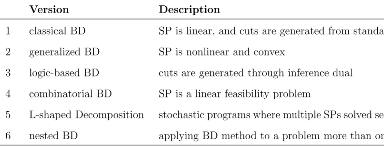
introduc-tion of the chapter as follows.

Version Description

1 classical BD SP is linear, and cuts are generated from standard dual 2 generalized BD SP is nonlinear and convex

3 logic-based BD cuts are generated through inference dual 4 combinatorial BD SP is a linear feasibility problem

5 L-shaped Decomposition stochastic programs where multiple SPs solved separately 6 nested BD applying BD method to a problem more than once

Table 5: Some versions of Benders’ Decomposition algorithm

5.1 Generalized Benders’ Decomposition

Many of todays real-world optimization problems involve nonlinear functions and con-straints. However, if the problem can be easily linearized or the nonlinearity arises only in the domain of the complicating variables, we can still apply classical BD to solve it. Otherwise, we must employ an extended BD method to tackle the problem.

It was A.M. Geoffrion (1972) who proposed the Generalized Benders’ Decomposition [13] which solves nonlinear problems where the SP is convex. Later in 2005, A.M. Costa [9] showed that it is also specifically appealing for nonconvex nonlinear problems which can be convexified after fixing a subset of variables.

Then in 1991 N. Sahinidis and I.E. Grossmann [29] observed that for MINLP problems the generalized BD method may not achieve a global or even a local optimum. Particularly, if the objective function and some of the constraints are nonconvex or if there exist nonlinear equations, the subproblem may not lead to a unique local optimum and the master problem may remove the global optimum. However, rigorous global optimization approaches can be adopted if the continuous terms are in a special structure like bilinear, linear fractional, concave separable. Thus, the main idea is to use convex envelopes to create lower-bounding