Planning in Discrete and Continuous Markov Decision Processes by Probabilistic Programming

Edinburgh Research Explorer

Planning in Discrete and Continuous Markov Decision Processes

by Probabilistic Programming

Citation for published version:

Nitti, D, Belle, V & Raedt, LD 2015, Planning in Discrete and Continuous Markov Decision Processes by Probabilistic Programming. in Machine Learning and Knowledge Discovery in Databases: European Conference, ECML PKDD 2015, Porto, Portugal, September 7-11, 2015, Proceedings, Part II. Lecture Notes in Computer Science, vol. 9285, Springer International Publishing, pp. 327-342. DOI: 10.1007/978-3-319-23525-7_20

Digital Object Identifier (DOI): 10.1007/978-3-319-23525-7_20 Link:

Link to publication record in Edinburgh Research Explorer Document Version:

Peer reviewed version

Published In:

Machine Learning and Knowledge Discovery in Databases

General rights

Copyright for the publications made accessible via the Edinburgh Research Explorer is retained by the author(s) and / or other copyright owners and it is a condition of accessing these publications that users recognise and abide by the legal requirements associated with these rights.

Take down policy

The University of Edinburgh has made every reasonable effort to ensure that Edinburgh Research Explorer content complies with UK legislation. If you believe that the public display of this file breaches copyright please contact [email protected] providing details, and we will remove access to the work immediately and investigate your claim.

Markov Decision Processes by

Probabilistic Programming

Department of Computer Science, KU Leuven, Belgium {davide.nitti,vaishak.belle,luc.deraedt}@cs.kuleuven.be

Abstract. Real-world planning problems frequently involve mixtures of continuous and discrete state variables and actions, and are formulated in environments with an unknown number of objects. In recent years, prob-abilistic programming has emerged as a natural approach to capture and characterize such complex probability distributions with general-purpose inference methods. While it is known that a probabilistic programming language can be easily extended to represent Markov Decision Processes (MDPs) for planning tasks, solving such tasks is challenging. Building on related efforts in reinforcement learning, we introduce a conceptually sim-ple but powerful planning algorithm for MDPs realized as a probabilistic program. This planner constructs approximations to the optimal policy by importance sampling, while exploiting the knowledge of the MDP model. In our empirical evaluations, we show that this approach has wide applicability on domains ranging from strictly discrete to strictly continuous to hybrid ones, handles intricacies such as unknown objects, and is argued to be competitive given its generality.

1

Introduction

Real-world planning problems frequently involve mixtures of continuous and discrete state variables and actions. Markov Decision Processes (MDPs) [28] are a natural and general framework for modeling such problems. However, while significant progress has been made in developing robust planning algorithms for discrete and continuous MDPs, the more intricate hybrid (i.e., mixtures) domains and settings with an unknown number of objects have received less attention.

The recent advances of probabilistic programming languages (e.g., BLOG [15], Church [6], ProbLog [10], distributional clauses [7]) has significantly im-proved the expressive power of formal representations for probabilistic models. While it is known that these languages can be extended for decision problems [27, 29], including MDPs, it is less clear if the inbuilt general-purpose inference system can cope with the challenges (e.g., scale, time constraints) posed by ac-tual planning problems, and compete with existing state-of-the-art planners.

In this paper, we consider the problem of effectively planning in domains where reasoning and handling unknowns may be needed in addition to cop-ing with mixtures of discrete and continuous variables. In particular, we adopt

dynamic distributional clauses (DDC) [17, 18] (an extension of distributional clauses for temporal models) to describe the MDP and perform inference. In such general settings, exact solutions may be intractable, and so approximate solutions are the best we can hope for. Popular approximate solutions include Monte-Carlo methods to estimate the expected reward of a policy (i.e., policy evaluation). Monte-Carlo methods provide state-of-the-art results in probabilis-tic planners [11, 9]. Monte-Carlo planners have been mainly applied in discrete domains (with some notable exceptions, such as [13, 1], for continuous domains). Typically, for continuous states, function approximation (e.g., linear regression) is applied. In that sense, one of the few Monte-Carlo planners that works in arbitrary MDPs with no particular assumptions is Sparse Sampling (SST) [8]; but as we demonstrate later, it is often slow in practice. We remark that most, if not all, Monte-Carlo methods require only a way to sample from the model of interest. While this property seems desirable, it prevents us from exploiting the actual probabilities of the model, as discussed (but unaddressed) in [9].

In this work, we introduce HYPE: a conceptually simple but powerful plan-ning algorithm for a given MDP in DDC. However, HYPE can be adapted for other languages, such as RDDL [22]. The proposed planner exploits the knowledge of the model via importance sampling to perform policy evaluation, and thus, policy improvement. Importance sampling has been used in off-policy Monte-Carlo methods [20, 25, 24], where policy evaluation is performed using trajectories sampled from another policy. We remark that standard off-policy Monte-Carlo methods have been used in reinforcement learning, which are es-sentially model-free settings. In our setting, given a planning domain, the pro-posed planner introduces a new off-policy method that exploits the model and works, under weak assumptions, in discrete, continuous, hybrid domains as well as those with an unknown number of objects.

We provide a detailed derivation on how the approximation is obtained using importance sampling. Most significantly, we test the robustness of the approach on a wide variety of probabilistic domains. Given the generality of our frame-work, we do not challenge the plan times of state-of-the-art planners, but we do successfully generate meaningful plans in all these domains. We believe this per-formance is competitive given the algorithm’s applicability. Indeed, the results show that our system at best outperforms SST [8] and at worst produces similar results, where SST is an equally general planner; in addition, it obtains reason-able results with respect to state-of-the-art discrete (probabilistic) planners.

2

Preliminaries

In a MDP, a putative agent is assumed to interact with its environment, de-scribed using a setS ofstates, a setAofactions that the agent can perform, a transition function p:S×A×S→[0,1], and areward function R:S×A→R.

That is, when in state sand on doinga, the probability of reaching s0 is given by p(s0 | s, a), for which the agent receives the reward R(s, a). The agent is taken to operate over a finite number of time stepst= 0,1, . . . , T, with the goal

of maximizing the expected reward: E[PTt=0γtR(st, at)], where s0 is the start state,a0the first action, andγ∈[0,1] is a discount factor.

This paper focuses on maximizing the reward in a finite horizon MDP; how-ever the same ideas are extendable for infinite horizons. This is achieved by computing a (deterministic) policyπ:S×D→A that determines the agent’s action at statesand remaining stepsd(horizon). The expected reward starting from statestand following a policy πis called thevalue function (V-function):

Vdπ(st) =E "_t+d X k=t γk−tR(sk, ak)|st, π # . (1)

Furthermore, the expected reward starting from statestwhile executing action atand following a policyπis called theaction-value function (Q-function):

Qπd(st, at) =E "t+d X k=t γk−tR(sk, ak)|st, at, π # . (2)

Since T =t+d, in the following formulas we will use T for compactness. An optimal policy π∗ is a policy that maximizes the V-function for all states. A sample-based planner uses Monte-Carlo methods to solve an MDP and find a (near) optimal policy. The planner simulates (by sampling) interaction with the environment in episodesEm_=<sm

0, am0, sm1, a1m, ..., smT, amT>, following some policyπ. Each episode is a trajectory ofT time steps, and we letsm

t denote the state visited at time t during episode m. (So, after M episodes,M ×T states would be explored). After or during an episode generation, the sample-based planner updatesQd(smt , amt ) for eachtaccording to a backup rule, for example, averaging the total rewards obtained starting from (sm_t , am_t ) till the end. The policy is improved using a strategy that trades-off exploitation and exploration, e.g., the -greedy strategy. In this case the policy used to sample the episodes is not deterministic; we indicate with π(at|st) the probability to select action at in state st under the policyπ. Under certain conditions, after a sufficiently large number of episodes, the policy converges to a (near) optimal policy, and the planner can execute the greedy policyargmaxaQd(s, a).

3

Dynamic Distributional Clauses

We assume some familiarity with standard terminology of statistical relational learning and logic programming [2]. We represent the MDP usingdynamic dis-tributional clauses[17, 7], an extension of logic programming to represent contin-uous and discrete random variables. Adistributional clause(DC) is of the form h∼ D ←b1, . . . ,bn, where thebiare literals and∼is a binary predicate written

in infix notation. The intended meaning of a distributional clause is that each ground instance of the clause (h∼ D ←b1, . . . ,bn)θdefines the random variable

hθ as being distributed according to Dθ whenever all the biθ hold, where θ is

a substitution. Furthermore, a term'(d) constructed from the reserved functor '/1 represents the value of the random variabled.

Example 1. Consider the following clauses:

n∼poisson(6). (3)

pos(P)∼uniform(1,10)←between(1,'(n),P). (4) left(A,B)← '(pos(A))>'(pos(B)). (5) Capitalized terms such as P,A and B are logical variables, which can be sub-stituted with any constant. Clause (3) states that the number of people n is governed by a Poisson distribution with mean 6; clause (4) models the position pos(P) as a random variable uniformly distributed from 1 to 10, for each person P such that P is between 1 and '(n). Thus, if the outcome of n is two (i.e., '(n) = 2) there are 2 independent random variablespos(1) andpos(2). Finally, clause (5) shows how to define the predicateleft(A,B) from the positions of any AandB. Ground atoms such asleft(1,2) are binary random variables that can be true or false, while terms such aspos(1) represent random variables that can take concrete values from the domain of their distribution.

Adistributional program is a set of distributional clauses (some of which may be deterministic) that defines a distribution over possible worlds, which in turn defines the underlying semantics. A possible world is generated starting from the empty setS =∅; for each distributional clauseh∼ D ←b1, ...,bn, whenever the

body{b1θ, ...,bnθ} is true in the setS for the substitutionθ, a valuev for the

random variablehθis sampled from the distributionDθand'(hθ) =vis added to S. This is repeated until a fixpoint is reached, i.e., no further variables can be sampled.Dynamic distributional clauses(DDC) extend distributional clauses in admitting temporally-extended domains by associating a time index to each random variable.

Example 2. Let us consider an object search scenario (objsearch) used in the experiments, in which a robot looks for a specific object in a shelf. Some of the objects are visible, others are occluded. The robot needs to decide which object to remove to find the object of interest. Every time the robot removes an object, the objects behind it become visible. This happens recursively, i.e., each new uncovered object might occlude other objects. The number and the types of occluded objects depend on the object covering them. For example, a box might cover several objects because it is big. This scenario involves an unknown number of objects and can be written as a partially observable MDP. However, it can be also described as a MDP in DDC where the state is the type of visible objects; in this case the state grows over time when new objects are observed or shrink when objects are removed without uncovering new objects. The probability of observing new objects is encoded in the state transition model, for example:

type(X)t+1∼val(T)← '(type(X)t) =T, not(removeObj(X)). (6)

numObjBehind(X)t+1∼poisson(1) ← '(type(X)t) =box,removeObj(X). (7)

type(ID)t+1∼finite([0.2:glass,0.3:cup,0.4:box,0.1:can])←

'(type(X)t) =box,removeobj(X),'(numObjBehind(X)t+1) =N,getLastID(Last)t,

Clause (6) states that the type of each object remains unchanged when we do not perform a remove action. Otherwise, if we remove the object, its type is removed from the state at timet+ 1 because it is not needed anymore. Clauses (7) and (8) define the number and the type of objects behind a boxX, added to the state when we perform a remove action onX. Similar clauses are defined for other types. The predicate getLastID(Last)_t returns the highest object IDin the state and is needed to make sure that any new object has a differentID. To complete the MDP specification we need to define a reward functionR(st, at), the terminal states that indicate when the episode terminates, and the applica-bility of an actionatis a statestas in PDDL. Forobjsearch we have:

stopt←'(type(X)t) =can.

reward(20)_t←stopt.

reward(−1)t←not(stopt).

That is, a state is terminal when we observe the object of interest (e.g., a can), for which a reward of 20 is obtained. The remaining states are nonterminal with reward −1. To define action applicability we use a set of clauses of the form

applicable(action)t←preconditionst.

For example, actionremoveobjis applicable for each object in the state, that is when its type is defined with an arbitrary valueType:

applicable(removeobj(X))t←'(type(X)t) =Type.

4

Planning by Importance Sampling

Our approach to plan in MDPs described in DDC is anoff-policy strategy [28] based on importance sampling and derived from the transition model. Related work is discussed more comprehensively in Section 5, but as we note later, sample-based planners typically only require a generative model (a way to gen-erate samples) and do not exploit the declarative model of the MDP (i.e., the actual probabilities) [9]. In our case, this knowledge leads to an effective plan-ning algorithm that works in discrete, continuous, hybrid domains, and domains with an unknown number of objects under weak assumptions.

In a nutshell, the proposed approach samples episodesEm_{and stores for each} visited statesm

t an estimation of theV-function (e.g., the total reward obtained from that state). The action selection follows an-greedy strategy, where theQ -function is estimated as the immediate reward plus the weighted average of the previously storedV-function points at timet+ 1. This is justified by the means of importance sampling as explained later. The essential steps of our planning system_Hype(=hybrid episodic planner) are given in Algorithm 1.

The algorithm realizes the following key ideas:

Algorithm 1_Hype

1: functionSampleEpisode(d, smt , m) .Horizond, states m

t in episodem 2: if d= 0then

3: return0

4: end if

5: foreach applicable actionainsmt do . Q-function estimation 6: Q˜md(s m t , a)←R(smt , a) +γ Pm−1 i=0 wiV˜di−1(sit+1) Pm−1 i=0 wi 7: end for

8: sampleu∼uniform(0,1) . -greedy strategy

9: if u <1−then 10: am t ←argmaxaQ˜ m d(smt , a) 11: else 12: am t ∼uniform(actions applicable insmt ) 13: end if 14: samplesm

t+1∼p(st+1|smt , amt ) .sample next state 15: Gmd ←R(s

m

t , amt ) +γ·SampleEpisode(d−1, smt+1, m) .recursive call 16: V˜dm(s m t )←G m d 17: store (smt ,V˜dm(smt ), d) 18: returnV˜dm(s m

t ) .V-function estimation forsmt at horizond 19: end function

– Lines 14-17 sample the next step and recursively the remaining episode of total lengthT, then stores the total discounted rewardGm

d starting from the current statesm

t . This quantity can be interpreted as a sample of the expectation in formula (1), thus an estimator of theV-function. For this and other reasons explained later,Gm

d is stored as ˜Vdm(smt ).

– Lines 8-13 implement an-greedy exploratory strategy for choosing actions.

– Most significantly, line 6 approximates theQ-function using theweighted av-erage of the stored ˜Vi

d−1(s i t+1) points: ˜ Qm_d (sm_t , a)←R(sm_t , a) +γ Pm−1 i=0 wiV˜di−1(sit+1) Pm−1 i=0 wi , (9)

wherewi _{is a weight function for episodeiat states}i

t+1. The weight exploits the transition model and is defined as:

wi= p(s i t+1|smt , a) q(si t+1) α(m−i). (10)

Here, for evaluating an actionaat the current statest,we letwibe the ratio of the transition probability of reaching a stored statesi

t+1and the probability used to samplesi_t+1, denoted usingq.Recent episodes are considered more significant than previous ones, and so α is a parameter for realizing this. We provide a detailed justification for line 6 below.

We note that line 6 requires us to go over a finite set of actions, and so in the presence of continuous action spaces (e.g., real-valued parameter for a move

action), we can discretize the action space or sample from it. More sophisticate approaches are possible [5, 26].

V91= 97

V2

9 = 98 V93= 90

s= (0,0)

a0 a00

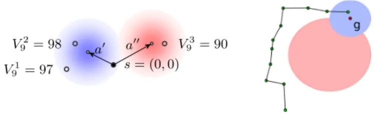
Fig. 1. Left: weight computation for the objpush domain. Right: a sampled episode that reaches the goal (blue), and avoids the undesired region (red).

Example 3. As a simple illustration, consider the following example called obj-push. We have an object on a table and an arm that can push the object in a set of directions; the goal is to move the object close to a point g, avoiding an undesired region (Fig. 1). The state consists of the object position (x, y), with push actions parameterized by the displacement (DX,DY). The state transition model is a Gaussian around the previous position plus the displacement:

pos(ID)t+1∼gaussian('(pos(ID)t)+ (DX,DY),cov)←push(ID,(DX,DY)). (11)

The clause is valid for any objectID; nonetheless, for simplicity, we will consider a scenario with a single object. The terminal states and rewards in DDC are:

stopt←dist('(pos(A)t),(0.6,1.0))<0.1.

reward(100)t←stopt.

reward(−1)t←not(stopt),dist('(pos(A)t),(0.5,0.8))>=0.2.

reward(−10)t←not(stopt),dist('(pos(A)t),(0.5,0.8))<0.2. (12)

That is, a state is terminal when there is an object close to the goal point (0.6,1.0) (i.e., distance lower than 0.1), and so, a reward of 100 is obtained. The nonterminal states have reward−10 whether inside an undesired region centered in (0.5,0.8) with radius 0.2, andR(st, at) =−1 otherwise.

Let us assume we previously sampled some episodes of lengthT = 10, and we want to sample them= 4-th episode starting froms0= (0,0). We compute

˜ Qm

10((0,0), a) for each action a(line 6). Thus we compute the weightswi using (10) for each stored sample ˜Vi

9(si1). For example, Figure 1 shows the computation of ˜Qm₁₀((0,0), a) for action a0 = (−0.4,0.3) and a00 = (0.9,0.5), where we have three previous samples i={1,2,3} at depth 9. A shadow represents the likeli-hoodp(si1|s0= (0,0), a) (left fora0 and right fora00). The weightwi(10) for each samplesi1 is obtained by dividing this likelihood byq(s1i) (withα= 1). Ifq(si1) is uniform over the three samples, samplei= 2 with total reward ˜V92(s21) = 98

will have higher weight than samplesi= 1 andi= 3. The situation is reversed for a00. Note that we can estimate ˜Qm_d (sm_t , a) using episodes i that may never encountersmt , atprovided thatp(sit+1|s

m

t , at)>0.

Computing the (Approximate) Q-Function

The purpose of this section is to motivate our approximation to the Q-function using the weighted average of the V-function points in line 6. Let us begin by expanding the definition of theQ-function from (2) as follows:

Qπ_d(st, at) =R(st, at)+γ

Z

st+1:T,at+1:T

Gd−1p(st+1:T, at+1:T|st, at, π)dst+1:T, at+1:T, (13)

where Gd−1 is the total (discounted) reward from time t+ 1 for d−1 steps: Gd−1 = P

d−1 k=1γ

k−1_R(s

t+k, at+k). Given that we sample trajectories from the target distributionp(st+1:T, at+1:T|st, at, π), we obtain the following approxima-tion to theQ-function equaling the true value in the sampling limit:

Qπ_d(st, at)≈R(st, at) + 1 Nγ X i Gi_d−1. (14)

Policy evaluation can be performed sampling trajectories using another policy, this is calledoff-policyMonte-Carlo [28]. For example, we can evaluate the greedy policy while the data is generated from a randomized one to enable exploration. This is generally performed using (normalized)importance sampling[25]. We let wi _{be the ratio of the target and proposal distributions to restate the sampling} limit as follows: Qπ_d(st, at)≈R(st, at) + 1 P wiγ X i wiGi_d−1. (15)

In standard off-policy Monte-Carlo the proposal distribution is of the form: p(st+1:T, at+1:T|st, at, π0) =

T−1

Y

k=t

π0(ak+1|sk+1)p(sk+1|sk, ak)

The target distribution has the same form, the only difference is that the policy is π instead of π0. In this case the weight becomes equal to the policy ratio because the transition model cancels out. This is desirable when the model is not available, for example in model-free Reinforcement Learning. The question is whether the availability of the transition model can be used to improve off-policy methods. This paper shows that the answer to that question is positive.

We will now describe the proposed solution. Instead of considering only tra-jectories that start from st, at as samples, we consider all sampled trajectories from timet+1 toT. Since we are ignoring steps beforet+1, the proposal distri-bution for sampleiis the marginal

p(st+1:T, at+1:T|s0, πi) =q(st+1)πi(at+1|st+1) T−1

Y

k=t+1

whereqis the marginal probabilityp(st+1|s0, πi). To compute ˜Qmd(smt , a) we use (15), where the weightwi (for 0≤i≤m−1) becomes the following:

p(sit+1|smt , a)πm(ait+1|sit+1) QT−1 k=t+1π m (aik+1|s i k+1)p(s i k+1|s i k, a i k) q(si t+1)πi(ait+1|sit+1) QT−1 k=t+1πi(a i k+1|s i k+1)p(s i k+1|s i k, a i k) = p(s i t+1|smt , a) q(si t+1) QT−1 k=t π m (aik+1|sik+1) QT−1 k=t πi(aik+1|sik+1) (16) ≈ p(s i t+1|smt , a) q(si t+1) α(m−i). (17)

Thus, we obtain line 6 in the algorithm given that ˜V_di₋₁(si_t) = Gi_d−1. In our algorithm the target (greedy) policyπm is not explicitly defined, therefore the policy ratio is hard to compute. We replace the unknown policy ratio with a quantity proportional toα(m−i)where 0< α≤1; thus, formula (16) is replaced with (17). The quantity α(m−i) becomes smaller for an increasing difference between the current episode indexmand thei-th episode. Therefore, the recent episodes are weighted (on average) more than the previous ones, as in recently-weighted averageapplied in on-policy Monte-Carlo [28]. This is justified because the policy is improved over time, thus recent episodes should have higher weight. Since we are performing policy improvement, each episode is sampled from a different policy. It has been shown [25, 20] that samples from different distribu-tions can be considered as sampled from a single distribution that is the mixture of the true distributions. Therefore, for a given episode

q(sit+1) = 1 N X j p(sit+1|s0, πj) = 1 N X j Z st Z at p(sit+1|st, at)p(st, at|s0, πj)dstdat ≈ 1 N X j p(sit+1|s j t, a j t),

where for eachjthe integral is approximated with a single sample (sj_t, aj_t) from the available episodes. Since each episode is sampled from p(s0:T, a0:T|s0, πj), samples (sjt, a

j

t) are distributed asp(st, at|s0, πj) and are used in the estimation of the integral.

The likelihoodp(si

t+1|smt , a) is required to compute the weight. This prob-ability can be decomposed using the chain rule, e.g., for a state with 3 vari-ables we have:p(si_t+1|s_tm, a) =p(v3|v2, v1, smt , a)p(v2|v1, smt , a)p(v1|s

m

t , a), where sit+1 ={v1, v2, v3}. In DDC this is performed evaluating the likelihood of each variable invi following the topological order defined in the DDC program. The target and the proposal distributions might be mixed distributions of discrete and continuous random variables; importance sampling can be applied in such distributions as discussed in [19, Chapter 9.8].

To summarize, for each state sm_t , Q(sm_t , at) is evaluated as the immediate reward plus the weighted average of stored Gi_d−1 points. In addition, for each state smt the total discounted reward Gmd is stored. We would like to remark that we can estimate theQ-function also for states and actions that have never

been visited, as shown in example 1. This is possible without using function approximations (beyond importance sampling).

Extensions

Our derivation follows a Monte-Carlo perspective, where each stored point is the total discounted reward of a given trajectory: ˜Vm

d (smt ) ← Gmd . However, following the Bellman equation, ˜Vm

d (s m

t )← maxaQ˜md (s m

t , a) can be stored in-stead. The Qestimation formula in line 6 is not affected; indeed we can repeat the same derivation using the Bellman equation and approximate it with impor-tance sampling: Qπd(st, at) =R(st, at) +γ Z st+1 Vdπ−1(st+1)p(st+1|st, at)dst+1 ≈R(st, a) +γ X wi P wiV˜ i d−1(s i t+1) = ˜Q m d(st, at), (18) withwi₌p(sit+1|st,at) q(si t+1) andsi

t+1the state sampled in episodeifor which we have an estimation of ˜V_di₋₁(si_t+1), while q(si_t+1) is the probability with which si_t+1 has been sampled. This derivation is valid for a fixed policy π; for a changing policy we can make similar considerations to the previous approach and add the term α(m−i). If we choose ˜V_di₋₁(sit+1)← Gid−1, we obtain the same result as in (9) and (17) for the Monte-Carlo approach. Instead of choosing between the two approaches we can use a linear combination, i.e., we replace line 16 with ˜Vm

d (s m

t )←λGmd + (1−λ)maxaQ˜md (s m

t , a). The analysis from earlier ap-plies by letting λ = 1. However, for λ = 0, we obtain a local value iteration step, where the stored ˜V is obtained maximizing the estimated ˜Qvalues. Any intermediate value balances the two approaches (this is similar to, and inspired by, TD(λ) [28]). Another strategy consists in storing the maximum of the two:

˜ Vm

d (smt ) ← max(Gmd , maxaQ˜md(smt , a)). In other words, we alternate Monte-Carlo and Bellman backup according to which one has the highest value. This strategy works often well in practice; indeed it avoids a typical issue in Monte Carlo methods: bad policies or exploration lead to low rewards, averaged in the estimated Q/V-function. For this reason it may occur that optimal actions are rarely chosen. The mentioned strategy avoids this, and a highvalue (line 9) is possible without affecting the performance.

5

Related work

There is an extensive literature on MDP planners, we will focus mainly on Monte-Carlo approaches. The most notable sample-based planners include Sparse Sam-pling (SST) [8], UCT [11] and their variations. SST creates a lookahead tree of depth D, starting from state s0. For each action in a given state, the algo-rithm samples C times the next state. This produces a near-optimal solution with theoretical guarantees. In addition, this algorithm works with continuous

and discrete domains with no particular assumptions. Unfortunately, the num-ber of samples grows exponentially with the depth D, therefore the algorithm is extremely slow in practice. Some improvements have been proposed [31], al-though the worst-case performance remains exponential. UCT [11] uses upper confidence bound for multi-armed bandits to trade off between exploration and exploitation in the tree search, and inspired successful Monte-Carlo tree search methods. Instead of building the full tree, UCT chooses the actionathat maxi-mizes an upper confidence bound ofQ(s, a), following the principle of optimism in the face of uncertainty. Several improvements and extensions for UCT have been proposed, including handling continuous actions [13] (see [16] for a review), and continuous states [1] with a simple Gaussian distance metric; however the knowledge of the probabilistic model is not directly exploited. For continuous states, parametric function approximation is often used (e.g., linear regression), nonetheless the model needs to be carefully tailored for the domain to solve [32]. There exist algorithms that exploit instance-based methods (e.g. [5, 26, 3]) for model-free reinforcement learning. They basically store Q-point estimates, and then use e.g., neighborhood regression to evaluateQ(s, a) given a new point (s, a). While these approaches are effective in some domains, they require the user to design distance metric that takes into account the domain. This is straightfor-ward in some cases (e.g., in Euclidean spaces), but it might be harder in others. We argue that the knowledge of the model can avoid (or simplify) the design of a distance metric in several cases, where the importance sampling weights and the transition model, can be considered as a kernel.

The closest related works include [25, 24, 20, 21], they use importance sam-pling to evaluate a policy from samples generated with another policy. Nonethe-less, they adopt importance sampling differently without the knowledge of the MDP model. Although this property seems desirable, the availability of the ac-tual probabilities cannot be exploited, apart from sampling, in their approaches. The same conclusion is valid for practically any sample-based planner, which only needs a sample generator of the model. The work of [9] made a similar statement regarding PROST, a state-of-the-art discrete planner based on UCT, without providing a way to use the state transition probabilities directly. Our algorithm tries to alleviate this, exploiting the probabilistic model in a sample-based planner via importance sampling.

For more general domains that contain discrete and continuous (hybrid) vari-ables several approaches have been proposed under strict assumptions. For ex-ample, [23] provide exact solutions, but assume that continuous aspects of the transition model are deterministic. In a related effort [4], hybrid MDPs are solved using dynamic programming, but assuming that transition model and reward is piecewise constant or linear. Another planner HAO* [14] uses heuristic search to find an optimal plan in hybrid domains with theoretical guarantees. However, they assume that the same state cannot be visited again (i.e., they assume plans do not have loops, as discussed in [14, sec. 5]), and they rely on the availability of methods to solve the integral in the Bellman equation related to the continuous part of the state. Visiting the same state in our approach is a benefit and not a

limit; indeed a previous visited states0 is useful to evaluateQd(s, a), when the weight is positive (i.e., whens0 is reachable fromswith actiona).

There exists several languages specific for planning, the most recent is RDDL [22]. A RDDL domain can be mapped in DDC and solved with HYPE. Nonethe-less, RDDL does not support a state space with an unknown number of variables as in Example 2. Some planners are based on probabilistic logic programming, for example DTProbLog [29] and PRADA [12], though they only support dis-crete action-state spaces. For domains with an unknown number of objects, some probabilistic programming languages such as BLOG [15], Church [6], and DC [7] can cope with such uncertainty. To the best of our knowledge DTBLOG [27] and [30] are the only proposals that are able to perform decision making in such domains using a POMDP framework. Furthermore, BLOG is one of the few languages that explicitly handles data association and identity uncertainty. The proposed paper does not focus on POMDP, nor on identity uncertainty; however, interesting domains with unknown number of objects can be easily described as an MDP that HYPE can solve.

Among the mentioned sample-based planners, one of the most general is SST, which does not make any assumption on the state and action space, and only relies on Monte-Carlo approximation. In addition, it is one of the few planners that can be easily applied to any DDC program, including MDPs with an un-known number of objects. For this reason SST was implemented for DDC and used as baseline for our experiments.

6

Experiments

This section answers the following questions: (Q1) Does the algorithm obtain the correct results? (Q2) How is the performance of the algorithm in different domains? (Q3) How does it compare with state-of-the-art planners?

The algorithm was implemented in YAP Prolog and C++, and run on a Intel Core i7 Desktop.

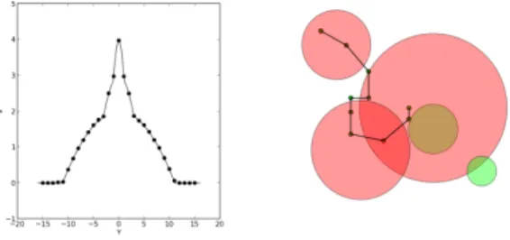
To answer (Q1) we tested the algorithm on a nonlinear version of the hybrid mars rover domain (calledsimplerover1) described in [23] for which the exactV -function is available (depthd= 3 and 2 variables: a two-dimensional continuous position and one discrete variable to indicate if the picture was taken). We choose 31 initial points and ran the algorithm for 100 episodes each. Each point took on average 1.4s. Fig. 2 shows the results where the line is the exactV, and dots are estimated V points. The results show that the algorithm converges to the optimalV-function with a negligible error. This domain is deterministic, and so, to make it more realistic we converted it to a probabilistic MDP adding Gaussian noise to the state transition model. The resulting MDP (simplerover2) is hard (if not impossible) to solve exactly. Then we performed experiments for different horizons, number of pictures points (1 to 4, each one is a discrete variable) and summed the rewards. For each instance the planner searches for an optimal policy and executes it, and after each executed action it samples additional episodes to refine the policy (replanning). The proposed planner is compared with SST

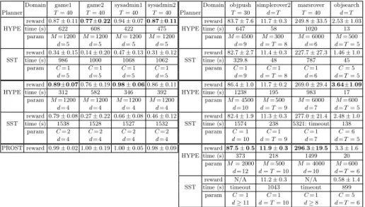
Table 1.Experiments: d is the horizon used by the planner,T the total number of steps,M is the maximum number of episodes sampled for HYPE, whileC is the SST parameter (number of samples for each state and action). Time limit of 1800s per instance. PROST results refer to IPPC2011.

Domain game1 game2 sysadmin1 sysadmin2 Planner T= 40 T= 40 T= 40 T= 40 HYPE reward 0.87±0.110.77±0.220.94±0.070.87±0.11 time (s) 622 608 422 475 param M= 1200 M= 1200 M= 1200 M= 1200 d= 5 d= 5 d= 5 d= 5 SST reward 0.34±0.15 0.14±0.20 0.47±0.13 0.31±0.12 time (s) 986 1000 1068 1062 param C= 1 C= 1 C= 1 C= 1 d= 5 d= 5 d= 5 d= 5 HYPE reward0.89±0.070.76±0.190.98±0.060.86±0.11 time (s) 312 582 346 392 param M= 1200 M= 1200 M= 1200 M= 1200 d= 4 d= 4 d= 4 d= 4 SST reward 0.79±0.08 0.27±0.22 0.66±0.08 0.46±0.12 time (s) 1538 1528 1527 1532 param C= 2 C= 2 C= 2 C= 2 d= 4 d= 4 d= 4 d= 4 PROST reward 0.99±0.02 1.00±0.19 1.00±0.05 0.98±0.09

Domain objpush simplerover2 marsrover objsearch Planner T= 30 d=T T= 40 d=T HYPE reward 83.7±7.6 11.7±0.3 249.8±33.5 2.53±1.03 time (s) 647 58 1020 13 param M= 4500 M= 300 M= 6000 M= 500 d= 9 d=T= 8 d= 6 d=T= 5 SST reward 82.7±2.7 11.4±0.3 227.7±27.3 1.46±1.0 time (s) 329.8 48 787 45 param C= 1 C= 1 C= 1 C= 5 d= 9 d=T= 8 d= 6 d=T= 5 HYPE reward 86.4±1.0 11.7±0.2 269.0±29.4 3.64±1.09 time (s) 1238 195 983 17 param M= 4500 M= 500 M= 6000 M= 600 d= 10 d=T= 9 d= 7 d=T= 5 SST reward 82.4±1.9 11.3±0.3 277.0±21.4 2.48±1.0 time (s) 1574 238 5321: timeout 138 param C= 1 C= 1 C= 1 C= 6 d= 10 d=T= 9 d= 7 d=T= 5 HYPE reward87.5±0.5 11.9±0.3 296.3±19.5 3.3±1.6 time (s) 373 218 1499 20 param M= 2000 M= 500 M= 4000 M= 600 d= 12 d=T= 10 d= 10 d=T= 6 SST

reward N/A 11.2±0.3 N/A 0.58±1.4 time (s) timeout 1043 timeout 899

param C= 1 C= 1 C= 1 C= 5

d≥11 d=T= 10 d≥8 d=T= 6

that requires replanning every step. The results for both planners are always comparable, which confirms the empirical correctness of HYPE (Table 1).

To answer (Q2) and (Q3) we studied the planner in a variety of settings, from discrete, to continuous, to hybrid domains, to those with an unknown number of objects. We performed experiments in a more realistic mars rover domain that is publicly available1, calledmarsrover (Fig. 2). In this domain we consider one robot and 5 picture points that need to be taken, the movement of the robot causes a negative reward proportional to the displacement and the pictures can be taken only close to the interest point. Each taken picture provides a different reward. Other experiments were performed in the continuousobjpush MDP described in Section 4 (Fig. 1), and in discrete benchmark domains of the IPPC 2011 competition. In particular, we tested a pair of instances of game of life and sysadmin domains. The results are compared with PROST [9], the IPPC 2011 winner, and shown in table 1 in terms of scores, i.e., the average reward normalizated with respect to IPPC 2011 results; score 1 is the highest result obtained, score 0 is the maximum between the random and the no operation policy.

As suggested by [9], limiting the horizon of the planner increases the perfor-mance in several cases. We exploited this idea for HYPE as well as SST ( sim-plerover2 excluded). For SST we were forced to use small horizons to keep plan time under 30 minutes. In all experiments we followed the IPPC 2011 schema,

1

that is each instance is repeated 30 times (objectsearch excluded), the results are averaged and the 95% confidence interval is computed. However, for every instance we replan from scratch for a fair comparison with SST. In addition, time and number of samples refers to the plan execution of one instance. The results (Table 1) highlight that our planner obtains generally better results than SST, especially at higher horizons. HYPE obtains good results in discrete do-mains but does not reach state-of-art results (score 1) for two main reasons. The first is the lack of a heuristic, that can dramatically improve the performance, indeed, heuristics are an important component of PROST [9], the IPPC winning planner. The second reason is the time performance that allows us to sample a limited number of episodes and will not allow to finish all the IPPC 2011 domains in 24 hours. This is caused by the expensiveQ-function evaluation; however, we are confident that heuristics and other improvements will significantly improve performance and results.

Finally, we performed experiments in theobjectsearch scenario (Section 3), where the number of objects is unknown. The results are averaged over 400 runs, and confirm better performance for HYPE with respect to SST.

Fig. 2. V-function for different rover positions (with fixed X= 0.16) in simplerover1

domain (left). A possible episode inmarsrover(right): each picture can be taken inside the respective circle (red if already taken, green otherwise).

7

Practical improvements

In this section we briefly discuss issues and improvements of HYPE. To evaluate the Q-function the algorithm needs to query all the stored examples, making the algorithm potentially slow. This issue can be mitigated with solutions used in instance-based learning, such as hashing and indexing. For example, in dis-crete domains we avoid multiple computations of the likelihood and the pro-posal distribution for samples of the same state. In addition, assuming policy improvement over time, only the Nstore most recent episodes are kept, since older episodes are generally sampled with a worse policy.

The algorithm HYPE relies on importance sampling to estimate the Q -function, thus we should guarantee thatp >0 ⇒q > 0, wherep is the target

and q is the proposal distribution. This is not always the case, like when we sample the first episode. Nonetheless we can have an indication of the estima-tion reliability. In our algorithm we use P

wi with expectation equals to the number of samples: E[Pwi] = m. If Pwi < thres the samples available are

considered insufficient to compute Qm_d(smt , a), thus action acan be selected to perform exploration.

A more problematic situation is when, for some actionat in some statest, we always obtain null weights, that isp(sit+1|st, at) = 0 for each of the previous episodesi, no matter how many episodes are generated. This issue is solved by adding noise to the state transition model, e.g., Gaussian noise for continuous random variables. This is equivalent to adding a smoothness assumption to the V-function. Indeed theQ-function is a weighted sum ofV-function points, where the weights are proportional to a noisy version of the state transition likelihood.

8

Conclusions

We proposed a sample-based planner for MDPs described in DDC under weak assumptions, and showed how the state transition model can be exploited in off-policy Monte-Carlo. The experimental results show that the algorithm produces good results in discrete, continuous, hybrid domains as well as those with an unknown number of objects. Most significantly, it challenges and outperforms SST. For future work, we will consider heuristics and hashing to improve the implementation.

References

1. Couetoux, A.: Monte Carlo Tree Search for Continuous and Stochastic Sequential Decision Making Problems. Thesis, Universit´e Paris Sud - Paris XI (2013) 2. De Raedt, L., Frasconi, P., Kersting, K., Muggleton, S. (eds.): Probabilistic

In-ductive Logic Programming, Theory and Applications, LNCS, vol. 4911. Springer (2008)

3. Driessens, K., Ramon, J.: Relational instance based regression for relational rein-forcement learning. In: Proc. ICML (2003)

4. Feng, Z., Dearden, R., Meuleau, N., Washington, R.: Dynamic programming for structured continuous Markov decision problems. In: Proc. UAI (2004)

5. Forbes, J., Andr´e, D.: Representations for learning control policies. In: Proc. of the ICML Workshop on Development of Representations (2002)

6. Goodman, N., Mansinghka, V.K., Roy, D.M., Bonawitz, K., Tenenbaum, J.B.: Church: A language for generative models. In: Proc. UAI. pp. 220–229 (2008) 7. Gutmann, B., Thon, I., Kimmig, A., Bruynooghe, M., De Raedt, L.: The magic

of logical inference in probabilistic programming. Theory and Practice of Logic Programming (2011)

8. Kearns, M., Mansour, Y., Ng, A.Y.: A Sparse Sampling Algorithm for Near-Optimal Planning in Large Markov Decision Processes. Machine Learning (2002) 9. Keller, T., Eyerich, P.: PROST: Probabilistic Planning Based on UCT. In: Proc.

10. Kimmig, A., Santos Costa, V., Rocha, R., Demoen, B., De Raedt, L.: On the Efficient Execution of ProbLog Programs. In: Logic Programming. LNCS, vol. 5366 (2008)

11. Kocsis, L., Szepesv´ari, C.: Bandit Based Monte-carlo Planning. In: Proc. ECML (2006)

12. Lang, T., Toussaint, M.: Planning with Noisy Probabilistic Relational Rules. Jour-nal of Artificial Intelligence Research 39, 1–49 (2010)

13. Mansley, C.R., Weinstein, A., Littman, M.L.: Sample-Based Planning for Contin-uous Action Markov Decision Processes. In: Proc. ICAPS (2011)

14. Meuleau, N., Benazera, E., Brafman, R.I., Hansen, E.A., Mausam, M.: A heuris-tic search approach to planning with continuous resources in stochasheuris-tic domains. Journal of Artificial Intelligence Research 34(1), 27 (2009)

15. Milch, B., Marthi, B., Russell, S., Sontag, D., Ong, D., Kolobov, A.: BLOG: Prob-abilistic Models with Unknown Objects. In: Proc. IJCAI (2005)

16. Munos, R.: From Bandits to Monte-Carlo Tree Search: The Optimistic Princi-ple Applied to Optimization and Planning. Foundations and Trends in Machine Learning, Now Publishers (2014)

17. Nitti, D., De Laet, T., De Raedt, L.: A Particle Filter for Hybrid Relational Do-mains. Proc. IROS (2013)

18. Nitti, D., De Laet, T., De Raedt, L.: Relational object tracking and learning. In: Proc. ICRA (2014)

19. Owen, A.B.: Monte Carlo theory, methods and examples (2013)

20. Peshkin, L., Shelton, C.R.: Learning from Scarce Experience. In: Proc. ICML. pp. 498–505 (2002)

21. Precup, D., Sutton, R.S., Singh, S.P.: Eligibility Traces for Off-Policy Policy Eval-uation. In: Proc. ICML (2000)

22. Sanner, S.: Relational Dynamic Influence Diagram Language (RDDL): Language Description, unpublished paper.

23. Sanner, S., Delgado, K.V., de Barros, L.N.: Symbolic Dynamic Programming for Discrete and Continuous State MDPs. In: Proc. UAI (2011)

24. Shelton, C.R.: Policy Improvement for POMDPs Using Normalized Importance Sampling. In: Proc. UAI. pp. 496–503 (2001)

25. Shelton, C.R.: Importance Sampling for Reinforcement Learning with Multiple Objectives. Ph.D. thesis, MIT (2001)

26. Smart, W.D., Kaelbling, L.P.: Practical Reinforcement Learning in Continuous Spaces. In: Proc. ICML (2000)

27. Srivastava, S., Russell, S., Ruan, P., Cheng, X.: First-order open-universe POMDPs. Proc. UAI (2014)

28. Sutton, R.S., Barto, A.G.: Reinforcement Learning: An Introduction. MIT Press (1998)

29. Van den Broeck, G., Thon, I., van Otterlo, M., De Raedt, L.: DTProbLog: A decision-theoretic probabilistic Prolog. In: Proc. AAAI (2010)

30. Vien, N.A., Toussaint, M.: Model-Based Relational RL When Object Existence is Partially Observable. In: Proc. ICML (2014)

31. Walsh, T.J., Goschin, S., Littman, M.L.: Integrating Sample-Based Planning and Model-Based Reinforcement Learning. In: proc. AAAI (2010)

32. Wiering, M., van Otterlo, M.: Reinforcement Learning: State-of-the-Art. Adapta-tion, Learning, and OptimizaAdapta-tion, Springer (2012)