(will be inserted by the editor)
MODELLING AND HIGH PERFORMANCE
SIMULATION OF ELECTROPHORETIC TECHNIQUES IN MICROFLUIDIC CHIPS
Pablo A. Kler · Claudio L. A. Berli · Fabio A. Guarnieri
Received: date / Accepted: date
Abstract Electrophoretic separations comprise a group of analytical tech-niques such as capillary zone electrophoresis, isoelectric focusing, isota-chophoresis and free flow electrophoresis. These techniques have been miniaturized in the last years and now represent one of the most im-portant applications of the lab-on-a-chip technology. A 3D and time-dependent numerical model of electrophoresis on microfluidic devices is presented. The model is based on the set of equations that governs elec-trical phenomena, fluid dynamics, mass transport and chemical reactions. The relationship between the buffer characteristics (ionic strength, pH) and surface potential of channel walls is taken into consideration. Numer-ical calculations were performed by using PETSc-FEM, in a Python en-vironment, employing high performance parallel computing. The method includes a set of last generation preconditioners and solvers, especially addressed to 3D microfluidic problems, which significantly improve the numerical efficiency in comparison with typical commercial software for multiphysics. In this work, after discussing two validation examples, the numerical prototyping of a microfluidic chip for two-dimensional elec-trophoresis is presented.
Pablo A. Kler
CIMEC, INTEC (UNL-CONICET), Santa Fe, Argentina. E-mail: [email protected]
Claudio L. A. Berli
INTEC (UNL-CONICET), G¨uemes 3450, 3000, Santa Fe, Argentina.
Dpto. F´ısico Matem´atica, FICH, UNL, Ciudad Universitaria, 3000, Santa Fe, Argentina. E-mail: [email protected]
Fabio A. Guarnieri
CIMEC, INTEC (UNL-CONICET), Santa Fe, Argentina. Fac. de Bioingenier´ıa, UNER, Oro Verde, Argentina. E-mail: [email protected]
Keywords Microfluidic chips · Electrophoresis · Numerical model · PETSc-FEM
1 Introduction
Electrophoretic separation techniques are based on the mobility of ions under the action of an external electric field. These techniques, which are widely used in chemical and biochemical analysis, have been miniatur-ized in the last 20 years and now represent one of the most important applications of lab-on-a-chip (LOC) technology (Manz et al., 1990; Lan-ders, 2007; Tian and Finehout, 2008). Electrophoretic separations carried out by LOC technology comprise a group of different techniques such as capillary zone electrophoresis (CZE), isoelectric focusing (IEF), iso-tachophoresis (ITP), moving boundary electrophoresis (MBE) and free flow electrophoresis (FFE) (Reyes et al., 2002; Peng et al., 2008; Wu et al., 2008). CZE, MBE and ITP are based on the displacement of elec-trophoretic species along the microchannel. IEF allows amphoteric com-ponent to focus at its stable isoelectric point (pI) in a predefined pH gradient (Sommer and Hatch, 2009). Free flow methods, such as FFE or free flow IEF (FFIEF), employ transverse electric fields in relation to the flow direction, allowing continuous operation and the possibility of connecting a second electrophoretic method. In fact, two-dimensional electrophoresis (2DE) are very demanded in proteins studies (Xu et al., 2005; Kohlheyer et al., 2008; Turgeon and Bowser, 2009). As microchips for electrophoresis are becoming increasingly complex, simulation tools are required to numerically prototype the devices, as well as to control and optimize manipulations (Erickson, 2005).
The first mathematical model of electrophoresis was developed by Sav-ille and Palusinski (1986). This 1D model is valid for monovalent analytes in a stagnant electrolyte solution, without electro-osmotic flow (EOF). More complex models of conventional electrophoresis were later reported (Hruska et al., 2006; Thormann et al., 2007; Bercovici et al., 2009). Nu-merical simulations aimed to LOC technology involving fluid flow and species transport were early addressed to electrokinetic focusing and sam-ple dispensing techniques (Patankar and Hu, 1998; Ermakov et al., 1998, 2000), by employing an algorithm based on finite volume method in a structured grid. Bianchi et al. (2000) performed 2D finite element method (FEM) simulations of EOF in T-shaped microchannels, taking into ac-count the inner part of the electric double layer (EDL). Arnaud et al. (2002) developed a FEM simulation of IEF for ten species, without con-sidering migration nor convection. Chatterjee (2003) developed a 3D fi-nite volume model to study several applications in microfluidics. More recently, Barz (2009) developed a fully-coupled model for electrokinetic
flow and migration in microfluidic devices employing 2D FEM. Differ-ent simulations of electrophoretic separations based on IEF techniques were presented by Hruska et al. (2006) and Thormann et al. (2007) in 1D domains, and by Shim et al. (2007) and Albrecht et al. (2007) in 2D domains.
Numerical simulations of electrophoretic separations in microfluidic chips represent a challenging problem from the computational point of view. Both the large difference among the relevant length scales involved and the multiphysics nature of the problem, lead to numerical difficulties: multiple nonlinear problems (each field requires a nonlinear calculation), excessive number of degrees of freedom, and ill-conditioning global matri-ces due to the high aspect ratios. Therefore, the implementation of parallel computations and advanced preconditioning, such as domain decompo-sition techniques, are crucial for the achievement of accurate numerical results and low computation times. Parallel computations and domain de-composition techniques in modelling electrokinetic flow and mass trans-port have not been extensively explored. Tsai et al. (2005) presented a 2D parallel finite volume scheme to solve EOF in L-shaped microchannels. 3D simulations of electrophoretic processes employing parallel calcula-tions were performed by Chau et al. (2008) for FFE using finite difference method, and by Kler et al. (2009) for CZE using FEM.
Here a 3D and time-dependent numerical model for electrophoretic processes in microfluidic chips is presented. The model can also work in 1D and 2D geometric domains, or stationary mode. Numerical cal-culations are carried out by using PETSc (Portable Extensible Toolkit for Scientific Computation)-FEM, in a Python environment. The method includes a set of last generation preconditioners and solvers, especially ad-dressed to 3D problems, which significantly improve numerical efficiency in comparison with typical software of multiphysics available for the pur-poses. As a matter of fact, the time required to complete the computation of a benchmark is reduced to less than 30%, as shown in the Electronic Supplementary Material (Online Resource 1). This advantage allows one to solve full, complex microfluidic problems, such as those found in nu-merical prototyping of state-of-the-art electrophoresis on chips.
Precisely, it is relevant to note that 3D simulations of the complete multiphysics problem of 2DE are not available in the literature, to the best of our knowledge. The closest approach to the subject is the work from Yang et al. (2008) that considers the transport of a single component sample in a 2D domain. Our model simulates transport, separation, and detection of several components (mixtures of more than 30 species), which undergo chemical reactions, in 3D domains.
In this paper, after presenting the mathematical modeling (Section 2), simulation tools (Section 3), and two validation examples (Sections
4.1 and 4.2), the numerical prototype of an electrophoretic chip involving FFIEF and CZE is discussed (Section 4.3).
2 Modelling
This section describes the mathematical model. First the fluid dynamics and the electric field are discussed, then the relationship between buffer composition and physicochemical properties of the channels wall is pre-sented, finally the mass transport balance for all species considered and the chemistry involved are described.
Isothermal conditions are assumed throughout this work. It is known that an important effect associated with electric current in microchannels is temperature rising due to internal heat generation, namely Joule effect (Li, 2004). Nevertheless, if the applied electric field is relatively low, and the microfluidic chip is able to reject the heat to the environment, the fluid temperature does not change appreciably (MacInnes et al., 2003; Berli, 2008; Kohlheyer et al., 2008).
2.1 Flow field
In the framework of continuum fluid mechanics, fluid velocityuand pres-surepare governed by the following equations (Probstein, 2003; Li, 2004):
−∇ ·u= 0, (1)
ρ(∂u
∂t +u· ∇u) =∇ ·(−pI+µ(∇u+∇u
T)) +ρg+ρ
eE . (2)
Equation 1 expresses the conservation of mass for incompressible flu-ids. Equation 2 expresses the conservation of momentum for Newtonian fluids of density ρ, viscosity µ, subjected to gravitational field of accel-eration g and electric field strengthE. The last term on the right hand side of Eq. 2 represents the contribution of electrical forces to the mo-mentum balance, where ρe = FPjzjcj is the electric charge density of
the electrolyte solution, obtained as the summation over all type-j ions, with valencezj and concentrationcj, andF is the Faraday constant.
2.2 Electric Field
The relationship between electric field and charge distributions in the fluid of permittivity is given by
∇ ·E=ρe. (3)
Modelling electrophoresis problems demands special considerations on the electric field, since it involves different contributions in the flow do-main, and is strongly affected by the presence of non-uniform electrolyte concentrations. Here we describe the computation of the electric field, as well the hypothesis included to simplify numerical calculations. For this purpose, a (η,τ) wall-fitted coordinate system is used, whereη andτ are, respectively, the coordinates normal and tangent to the solid boundaries. The first contribution to the electric field comes from the presence of electrostatic charges at solid-liquid interfaces. The interfacial charge has associated an electric potential ψ that decreases steeply in η-direction due to the screening produced by counterions and other electrolyte ions in solution, namely the EDL. The thickness of this layer is given by Debye lengthλD, which is on the order of 1−10nmfor the ionic concentrations
commonly used in electrophoresis. The value of ψ at the plane of shear is the electrokinetic potential ζ. Also in this modelling, ζ is allowed to vary smoothly along the τ-direction (see below Section 2.3) on a length scale L around 1cm. Nevertheless, since ζ/λD >> ζ/L, the variation of ψ withτ is disregarded and ψ is assumed to vary with η only.
There is also a potential φin the flow domain, which comes from the potential difference∆φexternally applied to drive electrophoresis and/or induce EOF. As the channel walls are supposed perfectly isolating, there are no components of the applied field normal to the wall, and φ varies inτ-direction only.
Therefore the total electric potential may be written as Φ(η, τ) =
ψ(η) +φ(τ). This superposition is valid if the EDL retains its equilibrium charge distribution when the electrolyte solution flows. The approxima-tion is part of the standard electrokinetic model (Hunter, 2001) and holds if the applied electric field (∼∆φ/L) is small in comparison with the EDL electric field (∼ζ/λD), which is normally the case in practice. Introducing
the electric fieldE=−∇Φinto Eq. 3 leads to the following expression,
∂2ψ ∂η2 + ∂2φ ∂τ2 =− ρe . (4)
The second term of this equation is non-null in electrophoresis prob-lems because the presence of concentration gradients in the fluid induces a variation of ∂φ∂τ along the channel. However, ∂∂τ2φ2 is several orders of mag-nitude lower than ∂∂η2ψ2 (see also MacInnes (2002); Sounart and Baygents (2007); Craven et al. (2008); Barz (2009)), which allows one to split the computation of the electric field in two parts, as explained below.
2.2.1 Electric double layer
According to the previous analysis, the EDL potential is governed by
∂2ψ
∂η2 =−
ρe
. Introducing the ion concentrationscjin the form of
Boltzmann-type distributions yields Poisson-Boltzmann model of the diffuse layer, which enables the calculation ofψ(η). This solution is useful to compute the EOF in nanochannels, or in microchannels with complicated geome-tries, such as sharp corners (Kler et al., 2009). Nevertheless, computa-tional requirements are very large when a whole chip is modelled. In this sense, and considering that the present work focuses on electrophoretic processes, here we simplify the calculation of the EOF by introducing the so-called thin EDL approximation (Brunet and Adjari, 2004; Berli, 2008): electro-osmosis is regarded as an electrically induced slip velocity in the direction of the applied electric field, the magnitude of which is given by Helmholtz-Smoluchowski equation,
u= ζ
µ∇φ. (5)
This approximation also implies that ρe ≈ 0 in the fluid outside the
EDL, meaning that the last term on the right-hand side of Eq. 2 is negligi-ble. Thus the electro-osmotic velocity enters the hydrodynamic field as a boundary condition, which significantly reduces computational demands. The simplification is appropriate taking into account thatλD ≈1−10nm,
while cross-sectional channel dimensions are 10−100µm.
2.2.2 Bulk fluid
Given the considerations made above, the electric potentialφ(τ) has to be calculated from the charge conservation equation in steady state (Prob-stein, 2003): ∇ ·(−σ∇φ−F N X j=1 zjDj∇cj +ρeu) = 0 (6)
where Dj is the diffusion coefficient, andσ is the electrical conductivity
of the electrolyte solution,
σ=F2 N X
j=1
zj2Ωjcj (7)
where Ωj is the ionic mobility. In fact, the terms between brackets in
fluxes due to fluid convection, electrical forces, and Brownian diffusion. Finally one may note that Eq. 6 reduces to ∂∂τ2φ2 = 0 (Laplace equation for the applied potential) only if electrolyte concentrations and mobilities are perfectly uniform.
2.3 Electrokinetic potential
In a typical IEF assay the pH changes several units along the channel, which induces a parallel variation of ζ, provided the interfacial charge has not been fully suppressed. In order to account for the influence of this variation on the EOF, here we include a model of ζ in terms of the pH and the ionic strength I = 12P
jzj2cj, which represents the total ion
concentrations of the bulk.
The electrokinetic potential at the solid-fluid interface depends on the charge generation mechanism of the surface (Hunter, 2001). In principle, it may be thought that solid walls expose toward the fluid a certain number of specific sites (nS) able to release or take H+ ions, with a dissociation
constant KS. In equilibrium with an aqueous electrolyte solution, the
surface becomes electrically charged. For the case of interfaces containing weak acid groups, such as silanol in fused silica capillaries and carboxyl in synthetic polymer materials, the following relationship is appropriate for symmetric monovalent electrolytes (Berli et al., 2003):
(8kBT INA)( 1 2)sinh( zeζ 2kBT ) = −ens 1 + 10(pKS−pH)e−eζ/kBT (8)
Therefore, if the parameters that characterize the interface are known (nS, KS), the ζ-potential can be readily predicted for different values
ofpH and I. Then the electro-osmotic velocity is directly coupled to the electrolyte composition. Empirical formulae ofζ(pH, I) were also reported in order to simplify calculations (Kirby, 2004).
2.4 Mass transport and chemistry
The mass transport of weakly concentrated sample ions and buffer elec-trolyte constituents can be modelled by a linear superposition of migra-tive, convective and diffusive transport mechanisms, plus a source term due to chemical reactions. In a non-stationary mode, the concentration of eachj-type species, is governed by (Probstein, 2003):
∂cj
were rj is the reaction term. Different electrolytes (acids, bases and
am-pholytes), analytes, and particularly the hydrogen ion have to be consid-ered. In electrolyte chemistry the processes of association and dissociation are much faster than the transport electrokinetic processes, hence, it is a good approximation to adopt chemical equilibrium constants to model the reactions of weak electrolytes (Arnaud et al., 2002), while strong elec-trolytes are considered as completely dissociated.
2.4.1 Acid-base reactions
For the general case, reactions associated to an ampholyteA are
AHFGGGGGGBA−+ H+ (10)
AH+2 FGGGGGGBAH + H+ (11)
then the equilibrium state is characterized by,
ka2 ka1 = [A −][H+] [AH] =Ka (12) kb2 kb1 = [AH][H +] [AH+2] =Kb (13)
where the square brackets represent concentration (mol/m3) of the given specie. The corresponding expressions ofrj are obtained as follows,
rA− =−ka1[A−][H+] +ka2[AH] (14) rAH=ka1[A−][H+]−ka2[AH]−kb1[AH][H+] +kb2[AH+2] (15) rAH+
2 =kb1[AH][H
+]−k
b2[AH+2] (16)
rH+=−ka1[A−][H+] +ka2[AH]−kb1[AH][H+] +kb2[AH+2] (17) In Eq. 17 the water dissociation term is not included due to the fact that this reaction is several orders of magnitude faster than reactions 10 and 11 (Arnaud et al., 2002), then [OH−] can be calculated directly as
[OH−] = Kw
[H+] (18)
2.4.2 Effective charge and mobility of analytes
When the concentration of analytes is much lower than that of buffer con-stituents, its effect on the pH is negligible. In these cases, considering all ionic species represents a high computational cost. However the influence of pH on the analytes must be taking into account. Thus the transport equation of these analytes includes rj = 0, and the product zjΩj as a
function of pH. For example, if the specie is an ampholyte that obeys a reaction scheme like the one shown in Eqs. 10 and 11,zjΩj is included in
Eq. 9 as an effective charge-mobility product (zef f(j)Ωef f(j); Chatterjee
(2003)). This product is calculated as (α0−α2)Ωj, whereα0 = [A−]/[AT]
and α2 = [AH2+]/[AT] with AT = [AH2+] + [AH] + [A
−], are the degrees of dissociation of anions and cations, respectively, which are written in terms of [H+] as, α0 = KaKb [H+]2 1 +[HKb+]+ KaKb [H+]2 (19) α2 = 1 1 +[HKb+]+ KaKb [H+]2 (20)
Therefore the governing equation for the sample plug results,
∂cj
∂t +∇ ·[−(α0−α2)Ωj∇φcj+ucj−Dj∇cj] = 0 (21)
where it is observed that the physical motion of analytes is coupled to the degree of dissociation at a given pH.
Previous works (Chatterjee, 2003; Shim et al., 2007) calculate the pH by using a nonlinear equation based on global electroneutrality, to avoid the solution of reactive terms and Eq. 9 for hydrogen ion. In parallel computing, solving monolithically two different nonlinear systems is dis-couraged due to its mathematical complexity (Storti et al., 2009) and computational inefficiency (Cai and Keyes, 2002).
Finally the reactive scheme (Eqs. 9 to 17) is used to solve species that change pH conditions, and the effective mobility scheme (rj = 0 and Eqs.
19 to 21) for those that cannot affect considerably the pH conditions. This scheme provides convergence, stability, and does not affect parallel calculations performance. Additionally the scheme allows to treat differ-ent reactive schemes, as enzymatic process or antigen-antibody systems, and different mobilities models.
3 Simulation Tools
3.1 Software
All numerical simulations presented were performed within a Python pro-gramming environment built uponMPI for Python (Dalc´ın et al., 2008),
PETSc for Python, and PETSc-FEM (Sonzogni et al., 2002). PETSc-FEM is a parallel multiphysics code primarily targeted to 2D and 3D finite elements computations on general unstructured grids. PETSc-FEM is based on MPI and PETSc (Balay et al., 2008), it is being developed since 1999 at the International Center for Numerical Methods in En-gineering (CIMEC), Argentina. PETSc-FEM provides a core library in charge of managing parallel data distribution and assembly of residual vectors and Jacobian matrices, as well as facilities for general tensor alge-bra computations at the level of problem-specific finite element routines. Additionally, PETSc-FEM provides a suite of specialized application pro-grams built on top of the core library but targeted to a variety of prob-lems (e.g., compressible/incompressible Navier–Stokes and compressible Euler equations, general advective-diffusive systems, weak/strong fluid-structure interaction). In particular mass transport, chemistry and fluid flow computations presented in this article were carried out within the Navier–Stokes module available in PETSc-FEM. This module provides the required capabilities for simulating mass transport and incompressible fluid flow through a monolithicSUPG/PSPG (Tezduyar et al., 1992; Tez-duyar and Osawa, 2000) stabilized formulation for linear finite elements. Electric field computations were carried out with the Charge Conserva-tion module, and transport equaConserva-tion was solved using the Electrophoresis module. Visualization and post-processing are carried out in Paraview 3.6 (Sandia and CSimSoft, 2000-2009).
In Online Resource 1 we compare the efficiency (computational time) of PETSc-FEM against a typical commercial software for multiphysics. A defined fluid dynamic problem is solved by using each method with the same hardware facilities.
3.2 Hardware
Simulations were carried out by using a Beowulf clusterAquiles (Storti, 2005-2008). The hardware consists of 82 disk-less single processor comput-ing nodes with Intel Pentium 4 Prescott 3.0GHz 2MB cache processors, Intel Desktop Board D915PGN motherboards, Kingston Value RAM 2GB DDR2 400MHz memory, and 3Com 2000ct Gigabit LAN network cards, interconnected with a 3Com SuperStack 3 Switch 3870 48-ports Gigabit Ethernet.
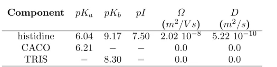
Component pKa pKb pI Ω D (m2/V s) (m2/s)
histidine 6.04 9.17 7.50 2.02 10−8 5.22 10−10
CACO 6.21 − − 0.0 0.0
TRIS − 8.30 − 0.0 0.0
Table 1: Physicochemical properties of analyte and buffer constituents (Palusinski et al., 1986; Chatterjee, 2003).
4 Validation and application examples
In what follows, three numerical examples of different electrophoretic sep-arations are presented: (1) a benchmark that consist in an IEF assay by immobilized pH gradient (IPG), (2) an IEF assay by ampholyte-based pH gradient, and (3) a 2DE assay involving FFIEF plus CZE. All numer-ical examples were solved neglecting gravitational forces, i.e. channels are supposed to be in horizontal position.
4.1 IEF by IPG
4.1.1 Stagnant fluid
In order to validate the model, an histidine IEF by IPG reported in the literature (Palusinski et al., 1986; Chatterjee, 2003) is reproduced here. The aminoacid histidine is focused in a straight channel (0.1 x 1.0 cm2). IPG is achieved by immobilizing cacodylic acid (CACO) and
tris(hydroxymethyl)-aminoetane (TRIS). Physicochemical parameters are summarized in Table 1.
Boundary conditions: a constant current density i= 0.2Am−2 is im-posed, this condition is attained by applying an appropriate potential difference ∆φ, which is instantaneously corrected with the actual value of σ. The anode is located at the left wall (x = 0.0 cm) of the channel, and cathode at the right wall (x= 1.0cm). The concentrations of CACO and TRIS are fixed in a linear way to obtain the pH profile, histidine flux through the up and bottom walls is set to zero.
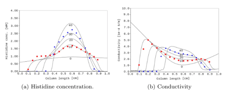
After the IPG is established, a sample of 1 mM histidine is injected in the whole channel. Then a constant current density i= 0.2Am−2 has to be imposed. Concentration of histidine and conductivity profiles at different times at the center of the channel are shown in Figs. 1a and 1b, respectively. The conductivity profile clearly shows the effect of the histidine concentration. During the focusing process conductivity follows the histidine concentration, decreasing considerably at channel ends. As a consequence, the electric field (which is directly coupled to conductivity
(a) Histidine concentration. (b) Conductivity
Fig. 1: Concentration and conductivity profiles along the channel at 0, 10, 20, 30 and 40 minutes. Full lines are the results of present work. Symbols corresponds to the values obtained by Palusinski et al. (1986); squares for 10 minutes and circles for 30 minutes.
by Eq. 6) raise at this regions, further increasing the focusing process. Results reasonably agree with those previously reported.
4.1.2 EOF effects
The previous example involved no bulk flow. In practice, this situation is hard to reach because the ζ-potential cannot be reduced to zero, and the resulting EOF has strong effects in focusing performance. Several attempts to quantify this effect were reported in the literature (Herr et al., 2000; Thormann et al., 2007). Here we simulate the histidine focusing problem with bulk flow due to the presence of EOF. The magnitude of the flow is related to the local electric field, wall electric properties and buffer solution composition, as described in Section 2. Calculations were carried out by using numerical values of the previous example (Table 1). Boundary conditions: apart from the conditions used in the previous example, here pressure is set to 0P a at the cathode, tangent velocity is set to 0 m/s at the anode and the cathode.As the calculation domain is 2D (x−y plane, see Fig. 2), the simulation implicitly assumes that the channel is considerably larger in the z direction that in they direction. Therefore, EOF slip velocity (Eq. 5) is included as the boundary condition at planesy= 0.0 cm and y= 0.1cm only.
In this case, due to the variation of pH along the channel, the wall
ζ-potential was modelled with Eq. 8. Parameters for this equation are:
pKs = 7.0 and ns = 1.22 1016+ 7.3 1016c0, where c0 is the local ion
concentration (Berli et al., 2003).
Figure 2 shows 2D plots of conductivity, electric field, pressure and fluid velocity, 2 minutes after the external potential is applied. A strong
coupling between these fields is observed. In fact, the fluid velocity is determined by both (i)ζ, which depends on pH and I, and (ii) E which in turn depends onσ (Figs. 2a and 2b). The superposition of these effects generates a non-uniform fluid velocity field along the channel (Fig. 2c) and the consequent pressure gradients (Fig. 2d). These non-uniformities are well known from ITP where electric field spatial variations due to conductivity gradients are important (Thormann et al., 2007). Here non-uniform ζ −potential effects are simulated without approximations. It is worth noting that previous works (Thormann et al., 2007; Herr et al., 2003) use an spatially averaged electro-osmotic velocity. Finally, under the conditions of this example, the influence of E(σ) prevails. Results shown in Fig. 2 are in agreement with experiments (Herr et al., 2003) and simulations(Thormann et al., 2007) reported in the literature. Focusing efficiency decreases due to the sample dispersion (non uniform transverse velocity profile) and the reduction of the sample residence time in the channel.
4.2 IEF by ampholyte-based pH gradient
Another way to implement IEF is by using a mixture of carrier am-pholytes, which naturally generates a pH gradient under the influence of an electric field. Further details on this technique can be found elsewhere (Landers, 2007; Sommer and Hatch, 2009). Here we simulate an IEF assay where the pH gradient is generated by ten ampholytes in solution. A 2D microchannel is modelled by a rectangle (0.01 x 1.0 cm2). Physicochemi-cal properties of the ampholyte (Table 2) were taken from the literature (Shim et al., 2007). Also in these calculations, Ω = 3 10−8 m2/V s and
D = 7.75 10−10 m2/s are used for all ampholytes. Initially ampholytes are uniformly distributed in the channel.
Boundary conditions: Potentials applied are 0V at the cathode (x = 0.0cm) and 100V at the anode (x= 1.0cm). Compounds fluxes through the walls is set to zero, except forH+ andOH− ions at the interfaces of anolyte and catholyte.
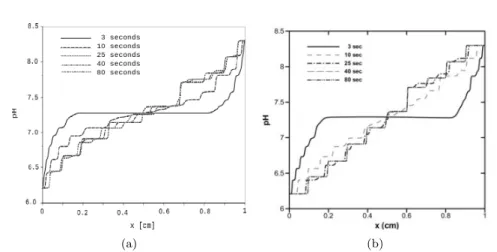
Figure 3a shows the pH gradient at different times, after applying the potential difference. Our predictions are compared to previous results (Fig. 3b). Unlike the IPG, ampholyte-based pH gradient has a strong transient behavior. After 80 s under the effect of the electric field, am-pholytes are focused around its pI, which yield different pH steps along the channel. The step-like shape is a consequence of the reduced number of ampholytes (Svensson, 1961).
(a)
(b)
(c)
(d)
Fig. 2: (a) conductivity, (b) electric field, (c) velocity and (d) pressure distributions at t= 2 minutes, for IEF with EOF.
Ampholyte pKa pKb pI 1 6.01 6.41 6.21 2 6.25 6.65 6.45 3 6.47 6.87 6.67 4 6.71 7.11 6.91 5 6.94 7.34 7.14 6 7.17 7.57 7.37 7 7.51 7.91 7.71 8 7.64 8.04 7.84 9 7.87 8.50 8.30 10 8.10 8.50 8.30
(a) (b)
Fig. 3: pH along the center of the channel for 3, 10, 25, 40 and 80 seconds. (a) Present work. (b) Shim et al. (2007). Copyright Wiley-VCH Verlag GmbH and Co. KGaA. Reproduced with permission.
4.3 2DE: FFIEF + CZE
Two-dimensional electrophoretic separations consist of two independent mechanisms that are employed sequentially. The separation efficiency is estimated as the product of the independent efficiency of each method, provided the methods are uncoupled (orthogonality). IEF and CZE sat-isfy orthogonality and have been extensively employed in the analysis of complex protein samples in conventional devices (Herr et al., 2003). FFIEF is a derivative of FFE, a classical technique in which an electric field is applied perpendicularly to a flowing sample solution, then ana-lytes are separated electrophoretically in a continuous flow (Xu et al., 2005; Kohlheyer et al., 2008; Turgeon and Bowser, 2009). In FFIEF, a pH gradient is generated across the channel.
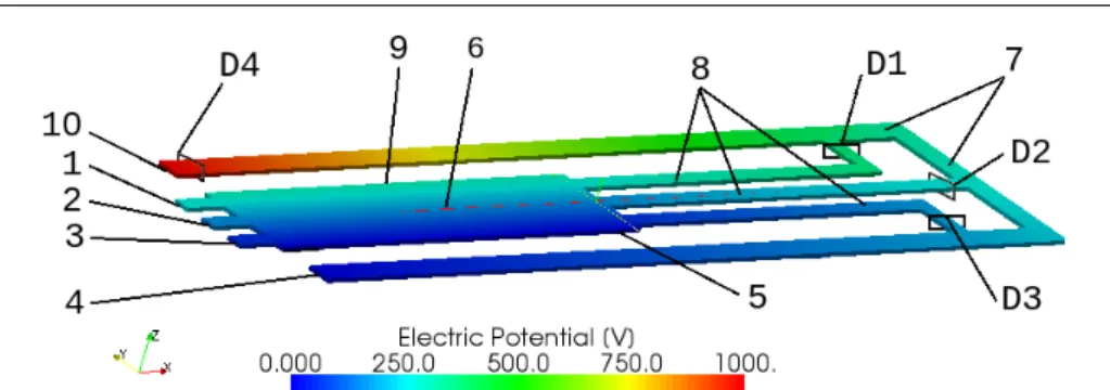
A 2DE separation involving FFIEF and CZE is simulated here. For this purpose, a microfluidic chip was designed following a FFIEF de-vice recently published (Kohlheyer et al., 2006). The geometry is pre-sented in Fig. 4. FFIEF is carried out in the FFIEF channel (10 x 3500 x 10000 µm3), then samples flow through three secondary channels (10 x 600 x 10000 µm3), and finally CZE is developed in the CZE channel (10 x 1000 x 50000 µm3). A main concern in 2DE separations is the uncoupling of the processes, which normally requires discontinuous oper-ation in order to avoid sample dispersions, mainly due to the geometry of turns or buffer heterogeneity (Tia and Herr, 2009). Here we adopt a continuous system, in which the mentioned effects do not influence the separation performance because the number of analytes is very low
com-pared with theoretical peak capacity of the device (Herr et al., 2003). In addition, electric field and conductivity gradients are sufficiently low to avoid flow instabilities (Posner and Santiago, 2006).
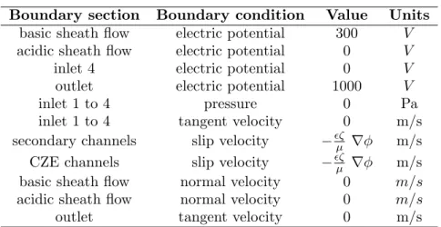
The fluid flow problem was solved by using Eqs. 1, 2, 5 and 6, and boundary conditions reported in Table 3, where ζ = 25 mV. The elec-tric potential at the initial state is shown in Fig. 4. The applied elecelec-tric potentials are fixed during the operation to provide the system with: a transverse electric field in the FFIEF channel, an axial electric field in the CZE channel, and EOF in the secondary and CZE channels.
The pH gradient for FFIEF is established by focusing twenty am-pholytes between two sheath flows of anolyte and catholyte, at pH 5.0 and 6.21, respectively. In these calculations, Ω = 3 10−8 m2/V s and
D= 7.75 10−10m2/sare used for all ampholytes. Other physicochemical properties of buffer components are listed in Table 4. Ampholytes 1 to 6 were injected continuously from inlet 1, ampholytes 7 to 14 from inlet 2, and ampholytes 15 to 20 from inlet 3 with a concentration of 1.0 mM. A more concentrated buffer (100 mM) at pH 4 is injected continuously from inlet 4. When ampholytes reach the CZE channel, they dilute into the buffer preserving pH 4. Stationary conditions are reached after 120s, where a linear-like pH gradient is formed (Fig. 5).
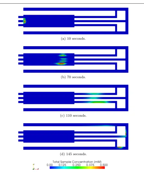
The separation of a mixture of 9 amphoteric compounds was simu-lated. Physicochemical properties of these analytes (see Table 5) were selected considering the mobilities and pIs of human aminoacids. All an-alytes were injected during 1.0 s from inlet 2 with a concentration of 0.1mM. Complete separation is achieved after 1000 seconds (real time). The computational time taken to complete the simulation is 40 hours. Analyte distributions during separation processes at different times are shown in Fig. 6.
A two-dimensional map of the separation is obtained from the in-formation provided by the four hypothetical detectors shown in Fig. 4. Detector 4 acquires the entire output signal (Fig. 7a), which is sectioned in three parts. These parts are obtained taking into account signals from detectors 1 to 3 , and assuming that areas under graphics are conserved. The first part of the signal has the same area that the signal of detector 1 and is assigned to the first pH range (5 to 5.4). The other parts of the signal are assigned to second and third pH ranges,respectively (5.4 to 5.8 and 5.8 to 6.2). The resulting plot is shown in Fig.7b. It is observed that the results of the numerical model can be easily presented in the graphic format that is customarily used in experiments of 2DE (Tia and Herr, 2009).
Boundary section Boundary condition Value Units
basic sheath flow electric potential 300 V
acidic sheath flow electric potential 0 V
inlet 4 electric potential 0 V
outlet electric potential 1000 V
inlet 1 to 4 pressure 0 Pa
inlet 1 to 4 tangent velocity 0 m/s
secondary channels slip velocity −ζµ ∇φ m/s
CZE channels slip velocity −ζµ ∇φ m/s
basic sheath flow normal velocity 0 m/s
acidic sheath flow normal velocity 0 m/s
outlet tangent velocity 0 m/s
Table 3: Boundary conditions for the electric field and fluid flow problems.
Ampholyte pKa pKb pI 1 4.90 5.30 5.10 2 4.95 5.35 5.15 3 5.00 5.40 5.20 4 5.05 5.45 5.25 5 5.10 5.50 5.30 6 5.15 5.55 5.35 7 5.20 5.60 5.40 8 5.25 5.65 5.45 9 5.30 5.70 5.50 10 5.35 5.75 5.55 11 5.40 5.80 5.60 12 5.45 5.85 5.65 13 5.50 5.90 5.70 14 5.55 5.95 5.75 15 5.60 6.00 5.80 16 5.65 6.05 5.85 17 5.70 6.10 5.90 18 5.75 6.15 5.95 19 5.80 6.20 6.00 20 5.85 6.25 6.05
Fig. 4: Geometry and electric potential distribution for initial state. 1, inlet 1;2, inlet 2;3, inlet 3;4, inlet 4 (CZE buffer inlet);5, basic sheath flow;6, FFIEF channel;7, ECZ channels;8, secondary channels;9, acidic sheath flow; 10, outlet. D1, D2, D3 and D4, are the locations for hy-pothetical detectors. Amphoteric pKa pKb pI Ω D analyte (m2/V s) (m2/s) 1 3.22 6.88 5.09 2.64 10−8 6.82 10−10 2 3.65 6.72 5.18 2.84 10−8 7.34 10−10 3 3.70 6.80 5.25 3.84 10−8 9.92 10−10 4 4.12 7.03 5.57 2.24 10−8 5.79 10−10 5 3.96 7.26 5.61 3.18 10−8 8.22 10−10 6 4.18 7.26 5.72 2.45 10−8 6.83 10−10 7 4.17 7.30 5.73 2.17 10−8 5.60 10−10 8 4.32 7.59 5.95 2.41 10−8 6.22 10−10 9 4.33 7.58 5.95 2.24 10−8 5.79 10−10 Table 5: Physicochemical properties of analyte constituents.
5 Summary and conclusions
A 3D and time dependent mathematical model for electrophoretic sepa-rations in microfluidic devices is presented. The model takes into account physicochemical property variations of buffer components and analytes, and its effects on fluid-solid interfaces, electric field and velocity profiles. Numerical implementation of the model is carried out by using FEM with parallel computing techniques, giving a powerful tool for simulations of electrophoretic separations in microfluidic chips.
In order to check the model, an IEF assay by IPG was simulated. Results agree with those previously reported (Palusinski et al., 1986). EOF effects in IEF assays were also analyzed. The model considers the coupling between buffer composition, flow field, electric field, and interface
(a)
(b)
Fig. 5: (a) pH in stationary conditions at z = 5.0 µm. (b) Ampholyte concentration and pH across the linera−rb atx= 8.0mm; z= 5.0µm.
property variations due to the electrolyte composition. Simulation of IEF by ampholyte-based pH gradient was also made as a second validation example. The predictions of the model successfully match previous results (Shim et al., 2007).
In all cases the method is much more efficient than similar software available commercially (Online Resource 1).
Finally, a 2DE was simulated: the separation of nine amphoteric com-pounds by means of FFIEF and CZE was studied. The successful sim-ulation of this complex system (3D, time-dependant, high aspect ratios in geometry, nonlinear fields) denotes the capability of the model to test and design state-of-the-art electrophoretic chips. Such a numerical proto-typing of 2DE had not reported before in the literature.
(a) 10 seconds.
(b) 70 seconds.
(c) 110 seconds.
(d) 145 seconds.
Fig. 6: Total sample distribution at 10, 70, 110 and 145 seconds
Caption of Electronic Supplementary Material
Efficiency of the numerical method proposed in comparison to a typical commercial software for multiphysics. A defined fluid dynamic problem is solved by using each method with the same hardware facilities.
(a) Detector 4. (b) Gel-like plot
Fig. 7: (a) Detector 4 signal, (b) Gel-like plot of the two-dimensional separation (FFIEF+CZE). Numbers 1 to 9 refer to analytes using de-nominations employed in Table 5.
Acknowledgements This work has received financial support from Consejo Nacional de In-vestigaciones Cient´ıficas y T´ecnicas (CONICET, Argentina), Universidad Nacional del Litoral (UNL, Argentina) and Agencia Nacional de Promoci´on Cient´ıfica y Tecnol´ogica (ANPCyT, Argentina). Authors made extensive use of freely distributed software as GNU/Linux OS, MPI, PETSc, GCC compilers, Paraview, Python, VTK, among many others.
References
Albrecht JW, El-Ali J, Jensen KF (2007) Cascaded free-flow isoelectric fo-cusing for improved fofo-cusing speed and resolution. Anal Chem 79:9364 – 9371
Arnaud I, Josserand J, Rossier J, Girault H (2002) Finite element simu-lation of off-gel buffering. Electrophoresis 23:3253–3261
Balay S, Buschelman K, Gropp WD, Kaushik D, Knepley MG, McInnes LC, Smith BF, Zhang H (2008) PETSc Web page. http://www.mcs. anl.gov/petsc
Barz DP (2009) Comprehensive model of electrokinetic flow and migra-tion in microchannels with conductivity gradients. Microfluid Nanofluid 7(2):249 –265
Bercovici M, Lele SK, Santiago JG (2009) Open source simulation tool for electrophoretic stacking, focusing, and separation. J Chromatogr A 1216:1008 – 1018
Berli CLA (2008) Equivalent circuit modeling of electrokinetically driven analytical microsystems. Microfluid Nanofluid 4(5):391 – 399
Berli CLA, Piaggio M, Deiber J (2003) Modeling the zeta potential of silica capillaries in relation to the background electrolyte composition. Electrophoresis 24:1587–1595
Bianchi F, Ferrigno R, Girault H (2000) Finite element simulation of an electroosmotic-driven flow division at a T-junction of microscale dimensions. Anal Chem 72(9):1987–1993
Brunet E, Adjari A (2004) Generalized Onsager relations for electroki-netic effects in anisotropic and heterogeneous geometries. Phys Rev E 69(1):016,306
Cai XC, Keyes DE (2002) Nonlinearly preconditioned inexact newton algorithms. SIAM J Sci Comput 24(1):183–200
Chatterjee A (2003) Generalized numerical formulations for multi-physics microfluidics-type applications. J Micromech Microeng 13:758–767 Chau M, Spiteri P, Guivarich R, Boisson H (2008) Parallel asynchronous
iterations for the solution of a 3d continuous flow electrophoresis prob-lem. Comput Fluid 37(9):1126–1137
Craven TJ, Rees JM, Zimmerman WB (2008) On slip velocity bound-ary conditions for electroosmotic flow near sharp corners. Phys Fluids 20(4):043,603
Dalc´ın L, Paz R, D’Elia MSJ (2008) MPI for Python: Performance im-provements and MPI-2 extensions. J Parallel Distr Com 68(5):655–662 Erickson D (2005) Towards numerical prototyping of labs-on-chip: model-ing for integrated microfluidic devices. Microfluid Nanofluid 1(4):301– 318
Ermakov S, Jacobson S, Ramsey J (1998) Computer simulations of elec-trokinetic transport in microfabricated channel structures. Anal Chem 70(21):4494–4504
Ermakov S, Jacobson S, Ramsey J (2000) Computer simulations of electrokinetic injection techniques in microfluidic devices. Anal Chem 72(15):3512–3517
Herr A, Molho J, Santiago J, Mungal M, Kenny T, Garguilo M (2000) Electroosmotic capillary flow with nonuniform zeta potential. Anal Chem 72:1053–1057
Herr A, Molho J, Drouvalakis K, Mikkelsen J, Utz P, Santiago J, Kenny T (2003) On-chip coupling of isoelectric focusing and free solution elec-trophoresis for multidimensional separarions. Anal Chem 75:1180–1187 Hruska V, Jaros M, Gas B (2006) Simul 5 - free dynamic simulator of
electrophoresis. Electrophoresis 27:984–991
Hunter R (2001) Foundations of Colloid Science, 2nd edn. Oxford Uni-versity Press
Kirby E Band Hasselbrink Jr (2004) Zeta potential of microfluidic sub-strates: 1. theory, experimental techniques, and effects on separations. Electrophoresis 25:187–202
Kler PA, L´opez EJ, Dalc´ın LD, Guarnieri FA, Storti MA (2009) High per-formance simulations of electrokinetic flow and transport in microflu-idic chips. Comput Method Appl M 198(30-32):2360 – 2367
Kohlheyer D, Besselink GAJ, Schlautmann S, Schasfoort RBM (2006) Free-flow zone electrophoresis and isoelectric focusing using a micro-fabricated glass device with ion permeable membranes. Lab Chip 6:374 – 380
Kohlheyer D, Eijkel JCT, van den Berg A, Schasfoort RBM (2008) Miniaturizing free-flow electrophoresis a critical review. Electrophore-sis 29(5):977 – 993
Landers JP (2007) Handbook of capillary and microchip electrophoresis and associated microtechniques, 3rd edn. CRC Press
Li D (2004) Electrokinetics in Microfluidics. Elsevier Academic Press MacInnes J, Du X, Allen R (2003) Prediction of electrokinetic and
pres-sure flow in a microchannel T-junction. Phys Fluids 15(7):1992–2005 MacInnes JM (2002) Computation of reacting electrokinetic flow in
mi-crochannel geometries. Chem Eng Sci 57(21):4539 – 4558
Manz A, Graber N, Widmer H (1990) Miniaturized total chemical analysis systems: A novel concept for chemical sensing. Sensor Actuat B 1:244–
248
Palusinski O, Graham A, Mosher R, Bier M, Saville D (1986) Theory of electrophoretic separations. part ii: Construction of a numerical scheme and its applications. AICHE J 32(2):215–223
Patankar N, Hu H (1998) Numerical simulation of electroosmotic flow. Anal Chem 70(9):1870–1881
Peng Y, Pallandre A, Tran NT, Taverna M (2008) Recent innovations in protein separation on microchips by electrophoretic methods. Elec-trophoresis 29(1):157–178
Posner JD, Santiago JG (2006) Convective instability of electrokinetic flows in a cross-shaped microchannel. Journal of Fluid Mechanics 555(-1):1–42
Probstein R (2003) Physicochemical Hydrodynamics. An Introduction, 2nd edn. Wiley-Interscience
Reyes D, Iossifidis D, Auroux P, Manz A (2002) Micro total analysis sys-tems. 1. introduction, theory, and technology. Anal Chem 74(12):2623– 2636
Sandia NL, CSimSoft (2000-2009) Paraview: Large data visualiztion.
http://www.paraview.org/
Saville D, Palusinski O (1986) Theory of electrophoretic separations. part i: Formulation of a mathematical model. AICHE J 32(2):207–214 Shim J, Dutta P, Ivory C (2007) Modeling and simulation of IEF in 2-D
microgeometries. Electrophoresis 28:572–586
Sommer G, Hatch A (2009) IEF in microfluidic devices. Electrophoresis 30:742–757
Sonzogni VE, Yommi AM, Nigro NM, Storti MA (2002) A parallel finite element program on a Beowulf cluster. Adv Eng Softw 33(7–10):427– 443
Sounart TL, Baygents JC (2007) Lubrication theory for electro-osmotic flow in a non-uniform electrolyte. J Fluid Mech 576(-1):139–172 Storti MA (2005-2008) Aquiles cluster at CIMEC. http://www.cimec.
org.ar/aquiles
Storti MA, Nigro NM, Paz RR, Dalc´ın LD (2009) Strong coupling strategy for fluid-structure interaction problems in supersonic regime via fixed point iteration. J Sound Vib 320(4-5):859 – 877
Svensson H (1961) Isoelectric fractionation, analysis, and characterization of ampholytes in natural pH gradients. I. The differential equation of solute concentrations at steady state and its solution for simple cases. Acta Chem Scand 15:325 – 341
Tezduyar T, Osawa Y (2000) Finite element stabilization parameters com-puted from element matrices and vectors. Comput Method Appl M 190(3-4):411–430
Tezduyar T, Mittal S, Ray S, Shih R (1992) Incompressible flow com-putations with stabilized bilinear and linear equal order interpolation velocity pressure elements. Comput Method Appl M 95:221–242 Thormann W, Caslavska J, Mosher R (2007) Modeling of electroosmotic
and electrophoretic mobilization in capillary and microchip isoelectric focusing. J Chromatogr A 1155(2):154 – 163
Tia S, Herr A (2009) On-chip technologies for multidimensional separa-tions. Lab Chip 9:2524–2536
Tian WC, Finehout E (2008) Microfluidics for Biological Applications, 1st edn. Springer
Tsai WB, Hsieh CJ, Chieng CC (2005) Parallel computation of electroos-motic flow in L-shaped microchannels. 6th World Congress of Struc-tural and Multiisciplinary Optimization pp 4971–4980
Turgeon RT, Bowser MT (2009) Micro free-flow electrophoresis: theory and applications. Anal Bioanal Chem 394(1):187 – 198
Wu D, Qin J, Lin B (2008) Electrophoretic separations on microfluidic chips. J Chromatogr A 1184(1-2):542 – 559
Xu Y, Zhang CX, Janasek D, Manz A (2005) Sub-second isoelectric fo-cusing in free flow using a microfluidic device. Lab Chip 3:224 – 227 Yang S, Liu J, DeVoe DL (2008) Optimization of sample transfer in