OpenBU http://open.bu.edu
Theses & Dissertations Boston University Theses & Dissertations
2017
Static and dynamic optimization
problems in cooperative
multi-agent systems
https://hdl.handle.net/2144/27013COLLEGE OF ENGINEERING
Dissertation
STATIC AND DYNAMIC OPTIMIZATION PROBLEMS
IN COOPERATIVE MULTI-AGENT SYSTEMS
by
XINMIAO SUN
B.S., Beijing Institute of Technology, 2012
M.S., Boston University, 2017
Submitted in partial fulfillment of the
requirements for the degree of
Doctor of Philosophy
2017
First Reader
Christos G. Cassandras, Ph.D.
Distinguished Professor of Engineering Professor and Head of Systems Engineering Professor of Electrical and Computer Engineering
Second Reader
Ioannis Ch. Paschalidis, Ph.D.
Professor of Electrical and Computer Engineering Professor of Systems Engineering
Professor of Biomedical Engineering
Third Reader
Calin Belta, Ph.D.
Professor of Mechanical Engineering Professor of Systems Engineering
Professor of Electrical and Computer Engineering Professor of Bioinformatics
Fourth Reader
Sean Andersson, Ph.D.
Associate Professor of Mechanical Engineering Associate Professor of Systems Engineering
My Ph.D. journey in the Control of Discrete-Event Systems Lab at Boston University is not only about doing research but also gaining courage and conquering fear in my life. Many people have provided me supports, assistance, and inspirations, without whom I would not be able to reach where I am right now.
First and foremost, I would like to express my deepest gratitude to my advisor, Prof. Christos G. Cassandras for patiently guiding me throughout the whole research process. His patience in guiding me to think critically, to find out key points from a simple case, to write good papers and to make good presentations is crucial for my research. This thesis would not have been possible without his thoughtful advice and mentorship. His passion towards research and pursuit of perfection will always inspire and motivate me.
Besides my advisor, I also sincerely thank the rest of my thesis committee mem-bers, Prof. Ioannis Paschalidis, Prof. Calin Belta and Prof. Sean Andersson, the committee chair Prof. Hua Wang, and Prof. David Castanon for their time, con-structive comments, guidance, ideas, and questions on my thesis and research. I would like to thank my collaborators Prof. Kagan Gokbayrak, Dr. Xiangyu Meng and Chao Zhang for their inspiring ideas and hard working.
I would also like to show my gratitude to the administrative staff in the Division of Systems Engineering and the Center for Information and Systems Engineering: Ms. Elizabeth Flagg, Ms. Cheryl Stewart, Ms. Denise Joseph and Ms. Christina Polyzos for the impeccable events they organized, the friendly atmosphere they created and all the great help they offered.
In addition, during my stay at Boston University, I have received much help from my fellow colleagues. I am thankful to my current and past CODES labmates, Yue Zhang, Nan Zhou, Rui Chen, Rebecca Swaszek, Arian Houshmand, Sepideh
for the rest of my BU family, Yu Xi, Liangxiao Xin, Feng Nan, Cristian-Ioan Vasile, Eran Simhon, Qi Zhao, Tingting Xu, Taiyao Wang. Many thanks to the seniors Yanfeng Geng, Yuting Chen, Yuting Zhang, Jing Wang, Wuyang Dai, Weicong Ding, Wei Si, Xiaodong Lan, Dingjiang Zhou, Hao Chen, TianSheng Zhang and Liang Li. With their own experiences, they helped me a lot.
I also would like to thank my roommates Yang Yu, Yuting Li, Wanying Zheng, Ouyang Guo and one of my best friend Cheng Cheng. They helped me to expand my knowledge, forget stress, and make life easier and beautiful.
Last but of course not least, I owe my deepest gratitude to my mother Guitao Hu and my father Gui Sun. Throughout my life, they unconditionally support me, believe me, and love me. I owe them more than I could repay in a lifetime. I am also grateful to my fiance Ruiqi Li for his support and love. He comforted me when I was upset, encouraged me when I was fearful, helped me no matter when I needed him. The happy time with him always reminds me how lucky I am. Many thanks to my grandfather who taught me calculation by abacus when I was 7 years old. Since then, calculation and math are my hobbies until now. I would also like to thank all the other family members and all my old friends for their consistent attention and support during all these years.
IN COOPERATIVE MULTI-AGENT SYSTEMS
XINMIAO SUN
Boston University, College of Engineering, 2017
Major Professor: Christos G. Cassandras, Ph.D.,
Distinguished Professor of Engineering,
Professor of Systems Engineering,
Professor of Electrical and Computer Engineering
ABSTRACT
This dissertation focuses on challenging static and dynamic problems encountered in cooperative multi-agent systems. First, a unified optimization framework is proposed for a wide range of tasks including consensus, optimal coverage, and resource alloca-tion problems. It allows gradient-based algorithms to be applied to solve these prob-lems, all of which have been studied in a separate way in the past. Gradient-based algorithms are shown to be distributed for a subclass of problems where objective functions can be decoupled.
Second, the issue of global optimality is studied for optimal coverage problems where agents are deployed to maximize the joint detection probability. Objective functions in these problems are non-convex and no global optimum can be guaranteed by gradient-based algorithms developed to date. In order to obtain a solution close to the global optimum, the selection of initial conditions is crucial. The initial state is determined by an additional optimization problem where the objective function is monotone submodular, a class of functions for which the greedy solution performance is guaranteed to be within a provable bound relative to the optimal performance.
exploiting the curvature information of the objective function. The greedy solution is subsequently used as an initial point of a gradient-based algorithm for the original optimal coverage problem. In addition, a novel method is proposed to escape a local optimum in a systematic way instead of randomly perturbing controllable variables away from a local optimum.
Finally, optimal dynamic formation control problems are addressed for mobile leader-follower networks. Optimal formations are determined by maximizing a given objective function while continuously preserving communication connectivity in a time-varying environment. It is shown that in a convex mission space, the connectivity constraints can be satisfied by any feasible solution to a Mixed Integer Nonlinear Programming (MINLP) problem. For the class of optimal formation problems where the objective is to maximize coverage, the optimal formation is proven to be a tree which can be efficiently constructed without solving a MINLP problem. In a mission space constrained by obstacles, a minimum-effort reconfiguration approach is designed for obtaining the formation which still optimizes the objective function while avoiding the obstacles and ensuring connectivity.
1 Introduction 1
1.1 Motivation and Background . . . 1
1.2 Research Outline and Literature Review . . . 6
1.2.1 Unified Optimization Framework of Multi-Agent Systems . . . 6
1.2.2 Optimal Coverage Problem . . . 7
1.2.3 Optimal Dynamic Formation Control Problem . . . 10
1.3 Contributions . . . 13
1.4 Dissertation Organization . . . 15
2 Unified Optimization Framework of Multi-Agent Systems 16 2.1 Introduction . . . 16
2.2 Problem Formulation . . . 17
2.2.1 Decomposition Theorem . . . 19
2.3 Examples of Multi-Agent Optimization Problems . . . 23
2.3.1 Consensus Problem . . . 23
2.3.2 Optimal Coverage Problem . . . 25
2.3.3 Counter-Example: Resource Allocation Problem . . . 30
2.4 Conclusions . . . 31
3 Optimal Coverage Problem 32 3.1 Introduction . . . 32
3.1.1 Submodularity-Based Approach . . . 32
3.1.2 Boosting Function Approach . . . 33
3.3 Distributed Gradient-Based Algorithm . . . 38
3.4 Submodularity-Based Approach . . . 39
3.4.1 Monotone Submodular Coverage Metric . . . 40
3.4.2 Greedy Algorithm and Lower Bounds . . . 43
3.4.3 Curvature Information Calculation . . . 45
3.4.4 Greedy-Gradient Algorithm . . . 48
3.4.5 Simulation Results . . . 51
3.5 Boosting Function Approach . . . 57
3.5.1 Structure of The Partial Derivative . . . 57
3.5.2 Boosting Function Approach . . . 61
3.5.3 Boosting Function Selection . . . 65
3.5.4 Simulation Results . . . 68
3.6 Conclusions . . . 71
4 Optimal Dynamic Formation Control 75 4.1 Introduction . . . 75
4.2 Problem Formulation . . . 76
4.3 Optimal Coverage Problem . . . 83
4.4 Optimal Dynamic Formation Control in a Mission Space with Obstacles 88 4.5 Simulation Results . . . 94
4.6 Conclusions . . . 98
5 Conclusions and Future Directions 100 5.1 Conclusions . . . 100
5.2 Future Directions . . . 102
A Mathematical Proofs 104 A.1 Proof of Equivalent Definitions . . . 104
References 113
Curriculum Vitae 119
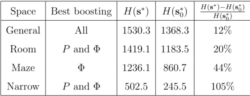
3.1 Summary of boosting function effects . . . 74
1·1 An example of a poor local optimum in optimal coverage problem . . 5
2·1 An example of mission space Ω with two obstacles and four agents in it. 18 2·2 Mission space with two polygonal obstacles . . . 27
2·3 Voronoi Partition by Lloyd algorithm (Cortes et al., 2004) . . . 30
3·1 Mission space with two polygonal obstacles . . . 36
3·2 Mission space example,FD consists of the blue dots . . . 39
3·3 T(c, N) andE(α, N) as a function of the number of agents N . . . . 46
3·4 Lower bound L(10) as a function of the sensing decay rate of agents . 49 3·5 Lower bound L(10) as a function of the sensing range of agents . . . 49
3·6 The decay factor λ= 0.02, and no obstacles in the mission space . . . 52
3·7 The decay factor λ= 0.12, and no obstacles in the mission space . . . 52
3·8 The decay factor λ= 0.4, and no obstacles in the mission space . . . 52
3·9 The decay factor λ= 0.02, and a wall-like obstacle in the mission space 53 3·10 The decay factor λ= 0.12, and a wall-like obstacle in the mission space 53 3·11 The decay factor λ= 0.4, and a wall-like obstacle in the mission space 53 3·12 The decay factor λ= 0.02, in a general mission space . . . 54
3·13 The decay factor λ= 0.12, in a general mission space . . . 54
3·14 The decay factor λ= 0.4, in a general mission space . . . 54
3·15 The decay factor λ= 0.02, in a maze mission space . . . 55
3·16 The decay factor λ= 0.12, in a maze mission space . . . 55
3·17 The decay factor λ= 0.4, in a maze mission space . . . 55 xiii
3·19 The decay factor λ= 0.12, in a room mission space . . . 56
3·20 The decay factor λ= 0.4, in a room mission space . . . 56
3·21 Mission space with two polygonal obstacles . . . 59
3·22 General obstacle with H(s∗0) = 1368.3 . . . 69
3·23 Room obstacle with H(s∗0) = 1183.5 . . . 69
3·24 Maze obstacle withH(s∗0) = 860.7 . . . 69
3·25 Narrow obstacle with H(s∗0) = 245.5 . . . 69
3·26 P-boosting function; H(s∗) = 1532.6 . . . 70 3·27 P-boosting function; H(s∗) = 1419.5 . . . 70 3·28 P-boosting function; H(s∗) = 1180.5 . . . 70 3·29 P-boosting function; H(s∗) = 502.5 . . . 70 3·30 Neighbor-boost, γ = 2, k = 500; H(s∗) = 1532.5 . . . 72 3·31 Neighbor-boost, γ = 1, g = 500; H(s∗) = 1415.1 . . . 72 3·32 Neighbor-boost, γ = 2,g = 1000; H(s∗) = 1168.6 . . . 72 3·33 Neighbor-boost, γ = 1,g = 300; H(s∗) = 245.3 . . . 72 3·34 Φ-boost, γ = 2, k = 1000;H(s∗) = 1526.4 . . . 73 3·35 Φ-boost, γ = 1, k = 1000;H(s∗) = 1419.1 . . . 73 3·36 Φ-boost, γ = 2, k = 100; H(s∗) = 1236.1 . . . 73 3·37 Φ-boost, γ = 2, k = 1000;H(s∗) = 502.5 . . . 73
4·1 A mission space example . . . 78
4·2 Optimal formation example 1 . . . 86
4·3 Optimal formation example 2 . . . 86
4·4 Illustration of networks . . . 90 4·5 Att= 0, an optimal formation is obtained by MINLP with H(s) = 741.5 96 4·6 The optimal formation in Fig. 4·5 is improved by CPA. H(s) = 816.7 96
4·8 Att= 6, agent 5 makes projection and CPA applies to Fig. 4·7 . . . 96
4·9 Att= 12, structure of the optimal formation changes . . . 97
4·10 At t= 35, the end of the mission . . . 97
4·11 A star-like connected graph . . . 97
4·12 Apply CPA to Fig. 4·11. H(s) = 781.1 . . . 97
A·1 Cartesian coordinate system . . . 107
A·2 Details of overlapping sensing areas . . . 107
A·3 Two Cartesian coordinate systems x−y and x0−y0 . . . 109
A·4 Agent h connects to agent 1 . . . 110
A·5 Agent h connects to agents 1 and 2 . . . 110
CPA . . . Connectivity Preservation Algorithm GGA . . . Greedy Gradient Algorithm
MINLP . . . Mixed Integer Nonlinear Programming
R2 . . . the Real plane
Chapter 1
Introduction
1.1
Motivation and Background
There exist many civilian and military missions involving searching, exploring and collecting data in an environment that is potentially highly dynamic, even hazardous to human operators (Hart and Martinez, 2006). Consider a scenario where rescue team members search for survivors after a catastrophic earthquake under the risk of aftershocks and landslides. Also think of the need of measuring environmental temperature, humidity, and gas concentration on wide complex areas in order to pro-vide more accurate weather forecast or prevent forest fire occurrence. More examples of such tasks include animal population studies, pollution detection, water and air quality monitoring.
It is desirable to develop autonomous multi-agent systems which are capable of dynamic self-deployment and communication in order to replace humans for poten-tially long unattended periods of operation. Indeed, many of the aforementioned tasks are difficult, or impossible, to be accomplished by a single agent. Multi-agent systems have significant advantages over a single sophisticated agent, including ro-bustness to dynamic uncertainties such as individual agent failures, non-stationary environments, and adversarial elements (Shamma, 2007; Wang and Zhang, 2017; Greco et al., 2010). The potential benefits of a multi-agent cooperative system have attracted the researchers’ attention in this field. In particular, consensus (Mesbahi and Egerstedt, 2010; Ji and Egerstedt, 2007; Moreau, 2004), formation control
(Ya-maguchi and Arai, 1994; Cao et al., 2011), containment control (Ji et al., 2008; Mei et al., 2012), vehicle-target assignment (Arslan et al., 2007; Nygard et al., 2001; Li and Cassandras, 2006), optimal coverage (Cortes et al., 2004; Cassandras and Li, 2005; Zhong and Cassandras, 2011; Gusrialdi and Zeng, 2011), maximum reward collection (Khazaeni and Cassandras, 2014), and persistent monitoring (Cassandras et al., 2013; Yu et al., 2015) are all well-known topics.
Cooperative multi-agent systems have the following features:
1. The system seeks to achieve a common goal which is determined by the agents’ states. The Individual agent may or may not have its goal.
2. Agents in the system may share their local information with each other through explicit communications, usually in the form of message passing over a network, or implicitly via observation of other agents’ states.
Considerable efforts have been dedicated to all aspects regarding the study of multi-agent cooperative systems including modeling of cooperative systems, resource allocation, discrete-event driven control, continuous and hybrid dynamical control, and theory of the interaction of information, control, and hierarchy. Methods, such as optimization and control approaches, emergent rule-based techniques, game theo-retic and team theotheo-retic approaches have been proposed. Performance measures that include the effects of hierarchies and information structures on solutions, performance bounds, concepts of convergence and stability, and problem complexity have also been put forward (Butenko et al., 2013).
In this dissertation, we focus on the optimization problems encountered in multi-agent systems. Optimization problems are often formulated by considering the com-mon goal as the objective, the states of agents as the decision variables, and the communication requirements as the constraints. These problems are static multi-agent problems if the decision variables are independent of time (e.g., deployment of
agents), for example, the vehicle-target assignment problem where multiple vehicles are going to be assigned to a number of targets by optimizing a certain total reward (Li and Cassandras, 2006). In addition, there are dynamic multi-agent problems in which the decision variables depend on time, that is, the states of the agents are optimized for a period of time which can be finite or infinite. Many types of trajec-tory optimization problems are good examples of dynamic multi-agent problems, such as persistent monitoring, data harvesting, and trajectory planning around obstacles (Khazaeni, 2016).
Optimal coverage problems are typical static optimization problems where agents are deployed in an environment to maximize the total coverage (Cortes et al., 2004; Cassandras and Li, 2005; Zhong and Cassandras, 2011; Gusrialdi and Zeng, 2011). One of the objective function is of the form
max
s H(s) =
Z
Ω
R(x)P(x,s)dx (1.1)
where x is a point in the mission space, R(x), x ∈ Ω is a prior information of the environment, e.g. event density function obtained from historical data, s is the posi-tion vector of the agents, and P(x,s) is the joint detection probability at x if agents are located at s. This objective function is shown to be of a surprisingly general nature, which motives us to pursue a unified optimization framework for multi-agent cooperative systems. Chapter 2 will discuss this topic in detail.
To solve optimization problems and perform tasks correctly and efficiently, we need to overcome the following difficulties:
1. Complexity and scalability. It is often impossible for an individual agent to access the information gathered by all agents. Furthermore, there is typically communication cost of gathering information in the centralized scheme. Even if information were available, the inherent complexity of the decision problems
cannot be ignored especially for a large-scale multi-agent system. Distributed algorithms are alternative approaches, which are used to speed up the compu-tation of complex computing tasks through parallel processing, and to make the system robust to the failure of agents. However, such benefits come with significant challenges, such as the analytical difficulties of dealing with partial in-formation and the trade-off between communication costs and the performance (Shamma, 2007).
2. Global optimality. The objective functions derived from the tasks are often non-convex and the environment is non-convex and may be time-varying. The inherent non-convexity of the objective function and environment uncertainty make a global optimum hard to be guaranteed by gradient-based methods. As we mentioned, though distributed algorithms are desired, it is impossible for us to identify whether there exist distributed algorithms only from the objective function like (1.1). We will then address the issue of identifying conditions under which a centralized solution to such problems can be recovered in a distributed manner in Chapter 2.
The issue of global optimality stands out for the optimal coverage problems espe-cially when the environment clutters with obstacles. For example, in a very simple scenario, two agents cover a mission space which is almost partitioned into a big area and a small area by an obstacle. Figure 1·1 shows a local optimum obtained by the gradient-based algorithm for such scenario where the blue rectangle represents an obstacle and the numbered circles 0 and 1 are agents. We can see no agent covers the big area, thus making the solution very bad. This motivates us to find a systematic way to obtain a local optimum with performance bound or to be able to escape a local optimum. Chapter 3 will study this problem.
Figure 1·1: An example of a poor local optimum in optimal coverage problem space, a static agent deployment solution may never give a satisfactory coverage of the whole space. In other words, there will always be a large uncovered area even with a globally optimal configuration. Under such scenarios, instead of assigning the agents to converge to some fixed locations, we can take advantage of the mobility of a mobile multi-agent system. However, communications between agents may be easily interrupted due to the mobility of the agents or be blocked by obstacles in the environment. The communication preservation is the first challenge to be considered, this motivates our third problem, optimal dynamic formation control, in Chapter 4.
This section is then followed by a brief outline of our research topics and literature review of start-of-the-art methods for the problems we present. Section 1.3 summa-rizes the main contributions of the dissertation and this chapter is ended by Section 1.4, which overviews the organization of the dissertation.
1.2
Research Outline and Literature Review
1.2.1 Unified Optimization Framework of Multi-Agent Systems
A unified optimization framework is proposed for static multi-agent problems includ-ing consensus, optimal coverage problems and resource allocation problems. They are usually treated as independent control problems and considerable progress has been made in a separate way.
Consensus or agreement problems require the states of all agents to reach an agreement (Ren et al., 2005; Mesbahi and Egerstedt, 2010; Ji and Egerstedt, 2007; Moreau, 2004). They have been studied extensively over the past decade, starting from single-integrator agents, to double-integrator agents, to identical general linear agents, and to non-identical general linear agents (Seyboth et al., 2016). Information exchange topology is assumed to be time-invariant or dynamic. Consensus protocol can either be continuous-time or discrete-time (Ren et al., 2005).
Coverage control is the process of controlling the movement of multiple agents and ultimately optimally deploying them in the mission space so as to maximize the sensing coverage or minimize the sum of distance from agents to the interested points in the mission (Zhong and Cassandras, 2011; Gusrialdi and Zeng, 2011; Sun et al., 2014; Cortes et al., 2004; Gusrialdi et al., 2008; Breitenmoser et al., 2010). This is a more general problem since the mission not only involves the agent-agent interactions like those in consensus and formation control, but also agent-environment interactions. Besides, the final states of agents in coverage control problems are needed to be found and optimized, instead of giving in advance like consensus and formation control problems. So we will focus on this problem in the following chapters and provide a detailed literature review in Section 1.2.2.
More recently, these problems tend to be solved via unified frameworks and algo-rithms. In (Nedi´c and Ozdaglar, 2009) and (Zhu and Martinez, 2013), a framework of
multi-agent non-convex optimization is proposed to minimize a sum of local objective functions subject to global constraints. However, the additive structure of this model is not always true, e.g., coverage control problems in (Zhong and Cassandras, 2011). In (Schwager et al., 2011), a generalized cost function is proposed to derive a stable gradient descent controller. In (Sakurama et al., 2015), on the other hand, the au-thors first come up with a distributed controller as a unified solution, then they find an objective function for a specific multi-agent coordination task. However, the as-sumption that the network topology is fixed may not be true due to agent failures and time-delays. In this dissertation, we propose a generalized optimization framework: to find the best states of agents so as to achieve a maximal reward (minimal cost) from the interactions between agents and the environment (e.g., coverage control) or among each other (e.g. consensus control).
Gradient-based methods are usually used to solve such problems (Bertsekas, 1995). Communication costs and constraints imposed on multi-agent systems, as well as the need to avoid single-point-of-failure issues, motivate distributed optimization schemes allowing agents to achieve optimality, each acting autonomously and with as little information as possible. A natural question is what kind of multi-agent optimization problems can be solved by a distributed gradient algorithm. In Chapter 2, we identify a subclass of problems where distributed gradient-based algorithms exist.
1.2.2 Optimal Coverage Problem
Coverage is a key performance metric of sensor networks and has been studied under various settings and approaches in the past decade (see (Fan and Jin, 2010) and (Zhu et al., 2012) for two surveys on the subject). Next, we give a synopsis of the literature that is most relevant to our work in this field.
The traditional coverage problem is of the form “How many agents are needed to be deployed or to be activated to cover a given region of interest?” Such
prob-lems are often solved using techniques in Computational Geometry. The probprob-lems of covering a set of points using a minimum number of a given geometric body are gen-erally NP-hard, and approximation algorithms had been proposed (Gonzalez, 1991; Hochbaum and Maass, 1985). More recently, it goes to a dual direction, i.e., how to deploy agents to maximize the rewards obtained by given number of agents in a bounded environment. The environment at first is assumed as a convex area with no obstacles in it (Cortes et al., 2004). Then it evolves to a non-convex area (Zhong and Cassandras, 2011), which makes it more complex. Optimal coverage problems can be solved by either on-line or off-line methods. Some widely used on-line methods, such as distributed gradient-based algorithms (Cassandras and Li, 2005; Zhong and Cassandras, 2011; Gusrialdi and Zeng, 2011) and Voronoi-partition-based algorithms (Cortes et al., 2004; Gusrialdi et al., 2008; Breitenmoser et al., 2010), typically result in locally optimal solutions, hence possibly poor performance. One normally seeks methods through which controllable variables escape from local optima and explore the search space of the problem aiming at better equilibrium points and, ultimately, a globally optimal solution. In heuristics algorithms, for example, simulated annealing (Laarhoven et al., 1987; Bertsimas and Tsitsiklis, 1993), this is done by probabilis-tically perturbing controllable variables away from a local optimum. However, it is infeasible for agents to perform such a random search which is notoriously slow and energy inefficient. Even if this method is used in a off-line setting, the computa-tion is inefficient and the condicomputa-tions for global optimality convergence are hard to be satisfied. A “ladybug exploration” strategy is applied to an adaptive controller in (Schwager et al., 2008), which aims at balancing coverage and exploration. How-ever, these on-line approaches cannot quantify the gap between the local optima they attain and the global optimum. In (Zhong and Cassandras, 2011), a gradient-based algorithm was developed to maximize the joint detection probability in a mission
space with obstacles.
Note that a proper starting point is crucial to get a good local optimum by gradient-based algorithms. Multiple-start algorithms (Snyman and Fatti, 1987; Mart´ı, 2003; Boese et al., 1994; Mart´ı et al., 2013) are proposed to address the global op-timization problem by using a local opop-timization routine but starting it from many different points. These methods have two phases that are alternated for a certain number of global iterations. The first phase generates a solution and the second seeks to improve the outcome. Each global iteration produces a solution that is typically a local optimum, and the best overall solution is the output of the algorithm. The most tricky thing is to create a balance between search diversification (structural variation) and search intensification (improvement).
We seek systematic methods to overcome the presence of multiple local optima in optimal coverage problems to avoid randomness and repeat work.
In computer science literature, a related problem is the “maximum coverage” problem (Khuller et al., 1999; Berman and Krass, 2002), where a collection of dis-crete sets is given (the sets may have some elements in common and the number of elements is finite) and at most N of these sets are selected so that their union has maximal size (cardinality). The objective function in the maximum coverage prob-lem is submodular and all properties of submodular maximization can be applied. Motivated by the maximum coverage works, we try to find out a good initial point with performance bound. in our work, we begin by limiting agents to a finite set of feasible positions. An advantage of this formulation is that it assists us in eliminat-ing obviously bad initial conditions for any gradient-based method. An additional advantage comes from the fact that we can show our coverage objective function to be monotone submodular, therefore, a suboptimal solution obtained by the greedy algorithm can achieve a performance ratio L(N)≥1− 1
agents in the system. The greedy solution is subsequently used as an initial point for a gradient-based algorithm to obtain solutions even closer to the global optimum.
In addition, the boosting function approach is proposed to escape a local optimum in a systematic way instead of randomly perturbing controllable variables away from a local optimum. This is accomplished by exploiting the structure of the problem considered. The main idea is to alter the regional objective function whenever an equilibrium is reached. A boosting function is a transformation of the associated partial derivative which takes place at an equilibrium point, where its value is zero; the result of the transformation is a non-zero derivative, which, therefore, forces an agent to move in a direction determined by the boosting function and to explore the mission space. When a new equilibrium point is reached, we revert to the original objective function and the gradient-based algorithm converges to a new (potentially better and never worse) equilibrium point.
1.2.3 Optimal Dynamic Formation Control Problem
Optimization problems of mobile multi-agent networks is a natural extension of the static multi-agent system to the mobile multi-agent system. For example, persistent monitoring problems are a dynamic version of the coverage control problem, consid-ering the case that the environment changes constantly and sometimes continuously. Persistent monitoring is defined as the problem of designing the optimal trajectories and finding the optimal movement along those trajectories (Cassandras et al., 2013; Yu et al., 2015; Lin and Cassandras, 2015).
The optimal dynamic formation control is motivated by coverage control problems with a fixed base where each agent is asked to maintain a connection with the base (Zhong and Cassandras, 2011). However, when the sensing area is small compared to the environment, the agent network cannot cover the whole mission space. In this dissertation, we deal with the issue that all agents are required to connect to a mobile
base, which is defined as a leader.
The optimal dynamic formation control is also motived by formation control prob-lems. In traditional formation control problems, mobile agents are required to estab-lish and maintain a certain spatial configuration, which is defined by relative distances or relative bearings (Cao et al., 2011; Oh and Ahn, 2014; Yamaguchi and Arai, 1994; Das et al., 2002). Formation control problems are generally approached in two ways: in the leader-follower setting, an agent is designated as a team leader moving on some given trajectory with the remaining agents tracking this trajectory while main-taining the formation; in the leaderless setting the formation must be maintained without any such benefit. In robotics, formation control is a well-studied problem. In (Yamaguchi and Arai, 1994), the desired shape for a strongly connected group of robots is achieved by designing a quadratic spread potential field on a relative dis-tance space. In (Desai et al., 1999), a leader and several followers move in an area with obstacles which necessitate the transition from an initial formation shape to a desired new shape; however, the actual choice of formations for a particular mission is not addressed in (Desai et al., 1999). In (Ji and Egerstedt, 2007) the authors consider the problem of connectivity preservation when agents have limited sensing and communication ranges; this is accomplished through a control law based on the gradient of an edge-tension function. More recently, in (Wang and Xin, 2013), the goal is to integrate formation control with trajectory tracking and obstacle avoidance using an optimal control framework.
Note that in these problems, the formations are usually given in advance. So the formation control seeks to deal with “How to go”. However, we should ask a high-level question “where to go” and/or “why this formation”. Since agent teams are typically assigned a mission, there is an objective (or cost) function associated with the team’s operation which depends on the spatial configuration (formation)
of the team. Therefore, in this dissertation, we view a formation as the result of an optimization problem which the agent team solves in either a centralized or distributed manner. We adopt a leader-follower approach, whereby the leader moves according to a trajectory that only he/she controls. During the mission, the formation is preserved or adapted if the mission (hence the objective function) changes or if the composition of the team is altered (by additions or subtractions of agents) or if the team encounters obstacles which must be avoided. In the latter case, in particular, we expect that the team adapts to a new formation which still seeks to optimize an objective function so as to continue the team’s mission by attaining the best possible performance. The problem is complicated by the fact that such adaptation must take place in real time. Thus, if the optimization problem determining the optimal formation is computationally demanding, we must seek a fast and efficient control approach which yields possibly suboptimal formations, but guarantees that the initial connectivity attained is preserved. Obviously, once obstacles are cleared, the team is expected to return to its nominal optimal formation.
Although the optimal dynamic formation control framework proposed here is not limited by the choice of tasks assigned to the team, we will focus on the dynamic coverage control problem because its static version is well-studied and amenable to efficient distributed optimization methods (Meguerdichian et al., 2001; Cortes et al., 2004; Cassandras and Li, 2005; Caicedo-Nuez and Zefran, 2008; Caicedo-Nunez and Zefran, 2008; Breitenmoser et al., 2010; Zhong and Cassandras, 2011; Gusrialdi and Zeng, 2011), while also presenting the challenge of being generally non-convex and sensitive to the agent locations during the execution of a mission. The local opti-mality issue, which depends on the choice of objective function, is addressed in (Sun et al., 2014; Schwager et al., 2008; Gusrialdi et al., 2013), while the problem of con-nectivity preservation in view of limited communication ranges is considered in (Ji
and Egerstedt, 2007; Zhong and Cassandras, 2011).
1.3
Contributions
To summarize, the main contributions of this dissertation are as follows.
For a unified optimization framework of multi-agent systems, the contributions are twofold. First, we build a general framework of multi-agent optimization problems taking both agent-agent interactions and agent-environment interactions into consid-eration. We integrate consensus, optimal coverage, and resource allocation problems in this framework. Second, we show that for some class of problems, each agent can decompose the objective function into a regional objective function dependent on this agent’s controllable states and a function independent of it. This implies a distributed algorithm and facilitates the evaluation of the partial derivative.
For optimal coverage problems, we address the issue of global optimality by proposing two approaches: submodularity-based approach and boosting function ap-proach. Submodularity-based approach adopts a simple greedy algorithm to get a solution with provable performance bound for an approximation problem where ob-jective function is monotone submodular. The bound is known to be within 1− 1
e of
the optimal solution. We derive a tighter lower bound for the optimal coverage prob-lems by further exploiting the structure of the objective function. In particular, we apply the total curvature and the elemental curvature of the objective function and show that these can be explicitly derived and lead to new and tighter lower bounds. Moreover, we show that the tightness of the lower bounds obtained through the total curvature and the elemental curvature respectively are complementary with respect to the sensing capabilities of the agents. In other words, when the sensing capabil-ities are weak, one of the two bounds is tight and when the sensing capabilcapabil-ities are strong, the other bound is tight. Thus, regardless of the sensing properties of our
agents, we can always determine a lower bound tighter than 1−1
e and, in some cases
very close to 1, implying that the greedy algorithm solution can be guaranteed to be near-globally optimal. The greedy solution is subsequently used as an initial point of a gradient-based algorithm to obtain solutions for the original optimal coverage problem.
In addition, the boosting function approach is proposed to escape a local optimum in a systematic way instead of randomly perturbing controllable variables away from a local optimum. This is accomplished by exploiting the structure of the problem considered. The main idea is to alter the regional objective function whenever an equilibrium is reached. A boosting function is a transformation of the associated partial derivative which takes place at an equilibrium point, where its value is zero; the result of the transformation is a non-zero derivative, which, therefore, forces an agent to move in a direction determined by the boosting function and to explore the mission space. When a new equilibrium point is reached, we revert to the original objective function and the gradient-based algorithm converges to a new (potentially better and never worse) equilibrium point. We define three families of boosting functions and discuss their properties.
For optimal dynamic formation control problems, the contribution is to formulate an optimization problem which jointly seeks to deploy agents in a two-dimensional mission space so as to optimize a given objective function while at the same time ensuring that the leader and remaining agents maintain a connected graph dictated by minimum distances between agents, thus resulting in an optimal formation. The minimum distances may capture limited communication ranges as well as constraints such as maintaining desired relative proximity between agents. We show that the so-lution to this problem guarantees such connectivity. For the class of optimal coverage control problems, we show that an optimal formation is a tree whose construction
is much more computationally efficient than that of a general connected graph. The formation becomes dynamic as soon as the leader starts moving along a trajectory which may either be known to all agents in advance or determined only by the leader. Thus, it is the team’s responsibility to maintain an optimal formation. We show that this is relatively simple as long as no obstacles are encountered. When one or more obstacles are encountered (i.e., they come within the sensing range of one or more agents), we propose a scheme for adapting with minimal effort to a sequence of new formations which maintain connectivity while still seeking to optimize the original team objective.
1.4
Dissertation Organization
In Chapter 2, we begin with a unified optimization framework for a wide range of tasks, including consensus, optimal coverage, and resource allocation problems. Gradient-based algorithms are shown to be distributed for a subclass of problems where objective functions can be decoupled.
In Chapter 3, we focus on the optimal coverage problems and propose two ap-proaches to address the issue of global optimality for the coverage control problems. In Chapter 4, we investigate the optimal dynamic formation control problems of mobile multi-agent systems. We propose algorithms for the convex mission space and non-convex one, respectively. We then focus on optimal coverage control problems and prove that a tree is an optimal formation, and propose an algorithm to construct such a tree in a convex mission space.
Finally, Chapter 5 summarizes the main contributions of the dissertation and discusses future research directions.
Chapter 2
Unified Optimization Framework of
Multi-Agent Systems
2.1
Introduction
Multi-agent systems are commonly modeled as hybrid systems with time-driven dy-namics describing the motion of the agents or the evolution of physical processes in a given environment, while event-driven behavior characterizes events that may occur randomly (e.g., an agent encounters an obstacle) or in accordance to control policies (e.g., an agent stopping to sense the environment or to change directions). In some cases, the dynamics of agents may be complex. From a design point of view, it is desirable to separate the control of the high-level multi-agent behavior from the low-level dynamical behavior of the agents. Optimization problems are often formulated to obtain the high-level multi-agent behavior, that is, tasks that multi-agent systems need to fulfill.
In this chapter, a unified optimization framework is proposed for a wide range of tasks including consensus, optimal coverage problems, and resource allocation prob-lems. It allows gradient-based algorithms to be applied to solve these problems, all of which have been studied in a separate way in the past. We then identify a subclass of problems that can be solved via distributed gradient algorithms by only investigating the structure of the objective function.
a general multi-agent optimization problem and point out a subclass of problems which can be solved by distributed gradient-based algorithms. In order to test the generality of this model, we show that consensus, optimal coverage problems, and resource allocation problems are all special cases of our framework in Section 2.3.
2.2
Problem Formulation
Consider a networked multi-agent system where agents are labeled by i ∈ A =
{1, . . . , N} in a mission space Ω. Let s = (s1, ..., sN) denote the global state
vec-tor. Considering mission space Ω may have obstacles or forbidden areas for agents, let F ⊆ Ω be the feasible state space for each agent, that is, si ∈ F. Let P(x,s) :
Ω×FN 7→Rbe a non-negativereward function to represent the reward resulting from interactions between agents with state s and x∈ Ω in the mission space. For exam-ple, in coverage control problems, P(x,s) is the joint detection probability of agents if some event occurs atx. For some pointx∈Ω, theproperty function R(x) : Ω7→R
describes the property associated with a point x in the mission space Ω, e.g., the weight of importance over the mission space Ω. We assume that R(x) ≥ 0, and
R
ΩR(x)dx < ∞. Still in coverage control problems, R(x) is a prior estimate of the frequency of event occurrences in the mission space. In a general setting, we seek to find the best state vectors= (s1, ..., sN) to maximize the total reward over the whole
mission space. maxH(s) = Z Ω R(x)P(x,s)dx s.t. si ∈F, i∈ A (2.1)
This is a general formulation because it models interactions between agents and the mission space, between agents and finite targets, and among agents. For example, Let Ω+ = {x | R(x) > 0} be a set for the points of interest and R(x) = 0 for the
Figure 2·1: An example of mission space Ω with two obstacles and four agents in it.
rest of points (e.g., obstacles in the mission space). The set Ω+ could be a compact set if it models the interactions between agents and a continuous mission space, a set with a finite number of points denoted by t = (t1, ...tM) if it models the finite
number of targets, or a set of agents themselvess. For the latter two cases,R(x) can be simplified toR(x) =PM
k=11(x−tk), andR(x) =
PN
i=11(x−si), respectively. For the objective function H(s) in the existing problems, we can find the corre-sponding P(x,s) and R(x). Examples can be found in Section 2.3.
Figure 2·1 shows a 2-d mission space with two obstacles and four agents in it. It is highly desirable to develop a distributed algorithm to solve (2.1) so as to (i) speed up the calculation by parallel computation by individual agents (ii) impart robustness to the system as a whole by avoiding single-point-of-failure issues.
However, it is not easy to see whether a distributed algorithm exist or not and it is natural to ask whether all kinds of problems in the form of (2.1) can be solved in a distributed fashion. If not, what characters should the problems have such that
distributed gradient based algorithms may exist.
2.2.1 Decomposition Theorem
There are different kinds of agent models regarding the ability that agents can interact with the mission space, targets or among agents. For example, if agents are sensors and their interaction with the mission space is sensing, the sensing ability could be unlimited, limited within a disk, or limited within a cone. We will show that the interacting ability model is crucial for a separable objective function H(s).
For the agent i, we assume that it interacts with the mission space in a limited
interaction region which is denoted by Vi, and Vi ⊆ Ω. Note that the region Vi can
vary with the state si. For example, an ultrasonic sensor can transmit and receive
ultrasound waves within a certain radius. Letpi(x, si) : Ω×F 7→Rbe a non-negative
local reward function to reflect the reward of the interaction between a pointx in the mission space and the agenti. For x∈Vi, the reward is a non-negative differentiable
functionfi(x, si). For x /∈Vi, the reward is a constantC (e.g., zero reward), which is
independent of si. In addition, we denote the non-interaction region as ¯Vi = Ω\Vi.
So the local reward function pi(x, si) is:
pi(x, si) =
fi(x, si) x∈Vi ⊂Ω
C x∈V¯i
(2.2) Generally speaking, fi 6=C for at least a finite set of points x∈ Vi. Besides, ¯Vi 6=∅
For simplicity, pi(x, si) is abbreviated to pi,fi(x, si) to fi in what follows.
We define Bi as a set of neighbor agents with respect toiand α is the cardinality
of the neighbor set.
Bi ={j :Vi∩Vj 6=∅}={b1i, ...b α
i}. (2.3)
Clearly, this set includes all agents j whose interaction region Vj has a nonempty
We define a regional state vector sL
i, α + 1 entries, including the states of the
neighbors and itself.
sLi = (si, sb1 i, ..., sb
α
i). (2.4)
Given that there is a total number of N agents, we define a complementary set Ci
with cardinality β.
Ci =A \ {Bi,{i}} (2.5)
The following theorem establishes the decomposition of H(s) into one function de-pending on sL
i , and the other one not depending on si, for any agent i∈ A.
Theorem 1 Given an objective function H(s), if there exist R(x) and local reward functions pi, i ∈ A as defined as (2.2) such that P(x,s) = P(p1, . . . , pN) and H(s)
can be expressed as H(s) = RΩP(p1, . . . , pN)R(x)dx, then the objective functionH(s)
can be expressed as two terms
H(s) =H1(siL) +H2(¯si) (2.6)
where ¯si = (s1, . . . , si−1, si+1, . . . , sn) for any i.
Proof: Since there exist pi defined in 2.2, the mission space Ω can be written
as Ω = Vi ∪ V¯i with respect to i, and Vi ∩V¯i = ∅. H(s) can be expressed as
H(s) =RΩP(p1, . . . , pN)R(x)dx. We can rewrite H(s) as the sum of two integrals:
H(s) = Z Ω P(p1, . . . , pN)R(x)dx = Z Vi R(x)P(p1, . . . , pN)R(x)dx+ Z ¯ Vi R(x)P(p1, . . . , pN)R(x)dx (2.7)
Recalling the definition of pi in (2.2), the first term is
Z
Vi
R(x)P(p1, . . . , fi, . . . , pN)dx. (2.8)
and (2.8) becomes Z Vi R(x)P (p1, . . . , fi, . . . , pN)dx− Z Vi R(x)P (p1, . . . , C, . . . , pN)dx + Z Vi R(x)P (p1, . . . , C, . . . , pN)dx, (2.9)
and the second term is
Z
¯
Vi
R(x)P(p1, . . . , C, . . . , pN)dx. (2.10)
Adding up (2.9) and (2.10), yields H(s)
H(s) = Z Vi R(x)P(p1, . . . , fi, . . . , pN)dx − Z Vi R(x)P(p1, . . . , C, . . . , pN)dx + Z Vi R(x)P(p1, . . . , C, . . . , pN)dx + Z ¯ Vi R(x)P(p1, . . . , C, . . . , pN)dx.
The integrands of the third and forth terms are the same. So the integral domain of these two terms can be summed to Ω and H(s) is
H(s) = Z Vi R(x) P (p1, . . . , fi, . . . , pN) −P(p1, . . . , C, . . . , pN) dx + Z Ω R(x)P (p1, . . . , C, . . . , pN)dx. (2.11)
si+1, . . . , sN) is a vector of all agent positions except i. Combining the definitions of
Bi and fi,H1(sLi) can be written as
H1(sLi) = Z Vi R(x) P pB1 i, . . . , pB α i, fi, C, . . . , C −P pB1 i, . . . , pB α i, C, C, . . . , C dx (2.12)
We name H1(sLi) as the regional objective function of agent i and observe that it
depends on Vi, fi, and pj for j ∈ Bi which are all available to agent i (the latter
through some communication with agents inBi). It’s nonzero in general sincefi 6=C.
The second term H2(¯si) is
H2(¯si) =
Z
Ω
R(x)P(p1, . . . , C, . . . , pN)dx. (2.13)
and it is independent of si in both integrand and integral domain.
Theorem 1 implies that for some problems in which the limited interaction abilities is proper defined, there exist distributed gradient-based algorithms such as
ski+1 =ski +ζk
∂H(s)
∂sk i
, k= 0,1, . . . (2.14) where the partial derivative with respect to agentican be calculated by only regional information it can access, i.e.,
∂H(s) ∂si = ∂H1(s L i ) ∂si . (2.15)
The step size sequence{ζk}is appropriately selected (see (Bertsekas, 1995)) to ensure
the convergence of the state.
Note that the definition of neighbors 2.3 is different from that defined based on a communication network. In a communication network, neighbors are agents who can communicate and the communication topology is usually fixed. In former case,
the neighbors of the agent i are time-varying. If the agent i’s neighbors are all the other agents, that is sL
i = s, then the first term H(sLi ) still depends on the whole
state vector. This is the worst case since agenti still needs all the states information and it is hard to avoid for a particular agent at some iterations by gradient-based algorithms. But this decomposition is still helpful if there exist some agent j such that sLj is a subset of s.
We also should point out that the exist ofpi defined in 2.2 is a sufficient condition
to decompose the objective function H(s). For example, if the objective function is
H(s) =s1 +s2, it is separable but there is no definition of pi needed.
2.3
Examples of Multi-Agent Optimization Problems
In this section, we illustrate how the general problem setting (2.1) and Theorem 1 can be specialized to coverage control problems, consensus control and a counter-example resource allocation problem proposed in (Zhu and Martinez, 2013).
2.3.1 Consensus Problem
Consensus or agreement problem of a multi-agent system requires all agents to reach the same state, i.e., s1 =...=sN. These problems are usually addressed in a control
viewpoint, i.e., propose a control law such that the states of agents converge to a same state. Examples of consensus algorithms may be found in (Mesbahi and Egerstedt, 2010; Ji and Egerstedt, 2007; Moreau, 2004).
LetG= (N, E) be a graph that specifies the communication topology of a network ofN agents whereN is the agent set andE ={(i, j) :i, j ∈ N }contains all connected agent pairs is the edge set. The graph is full connected. A consensus algorithm usually
are expressed in the form of a linear system ˙ si(t) = X j∈Ni [sj(t)−si(t)], s(0) =c (2.16)
where Ni is the neighbor set of agent i such that (i, j)∈E.
The consensus problem can be shown to fit the general framework We can consider the objective function H(s) to be
H(s) = 1 2
X
(i,j)∈E
||sj −si||2 (2.17)
From the objective function value view, the optimal value is zero and it is obtained when s1 =...=sN. That’s exactly the solution of the consensus problem. From the
partial derivative view, the partial derivative of H(s) in (2.17) with respect to si is
∂H(s)
∂si
= X
j∈Ni
(sj −si) (2.18)
is also exactly the same as the usual distributed consensus algorithm, see (Mesbahi and Egerstedt, 2010; Ji and Egerstedt, 2007; Moreau, 2004).
Although it’s obvious to see that for some agent i, H(s) defined in 2.17 can be decoupled into two terms
H1(sLi) = 1 2 X j∈Ni ||sj−si||2 (2.19) and H2(¯si) = 1 2 X (k,m)∈E,k,m6=i,Ni ||sk−sm||2 (2.20)
Note that Ni is a finite set, we can set R(x) to be R(x) = N X j=1 1(x−sj). (2.21)
For each agent i, there exist a local objective function
pi(x, si) = 1 2kx−sik 2 x=s j, j ∈ Ni, j > i 0 others. (2.22)
and the total rewardP(x,s) is a sum of pi(x, si)
P(x,s) = 1 2 N X i=1 pi(x, si) (2.23)
The objective function is
H(s) = Z Ω P(x,s) N X j=1 1(x−sj)dx = 1 2 Z Ω N X j=1 N X i=1 pi(x, si)1(x−sj)dx = 1 2 N X i=1 X j∈Ni,j>i ||sj−si||2 = 1 2 X (i,j)∈E ||sj−si||2 (2.24)
2.3.2 Optimal Coverage Problem
We introduce two kinds of coverage control modeling frameworks. To distinguish them, we name them optimal coverage and Voronoi-based coverage, respectively.
Optimal Coverage
In optimal coverage problems, agents (e.g., sensors) sense the environment to detect some events happening in it. Our goal is to control the agent position vector s =
(s1, . . . , sN) to maximize the overall joint detection probability of events taking place
in the environment.
The mission space Ω is modeled as a non-self-intersecting polygon, i.e., a polygon such that any two non-consecutive edges do not intersect. The mission space may contain obstacles which are modeled as m non-self-intersecting polygons denoted by
Oj, j = 1, . . . , m which block the movement of agents. The interior of Oj is denoted
by ˚Oj and thus the overall feasible space is F = Ω\( ˚O1∪. . .∪O˚m), i.e., the space
Ω excluding all interior points of the obstacles. We assume that each such agent has a bounded sensing range defined by the sensing radius δi. Thus, the sensing region
of agent i is Ωi ={x: di(x)≤δi}where di(x) =kx−sik. The presence of obstacles
inhibits the sensing ability of an agent, making a visibility set for agent i V(si)⊂F.
A point x ∈ F is visible from si ∈ F if the line segment defined by x and si is
contained in F, i.e., [λx+ (1−λ)si] ∈F for all λ ∈ [0,1], and x can be sensed, i.e.
x∈ Ωi. Then, Vi = Ωi ∩ {x: [λx+ (1−λ)si] ∈F} is a set of points in F which are
visible fromsi. We also define ¯V(si) = F \Vi to be the invisibility set (e.g., the grey
area in Figure 2·2).
A sensing model for any agentiis given by the probability that idetects an event occurring at x ∈ Vi, denoted by fi(x, si). We assume that fi(x, si) is expressed as
a function of di(x) = kx−sik and is monotonically decreasing and differentiable in
di(x). An example of such a function is
fi(x, si) =p0ie−λikx−sik
mission space
Obstacle
Obstacle
overall sensing detection probability is denoted as pi(x, si) and defined as pi(x, si) = fi(x, si) if x∈Vi 0 if x∈V¯(si) (2.25)
Note thatfi(x, si) is not a continuous function ofsi and that this is the concrete form
of local reward function in (2.2). We may now define the joint detection probability
that an event at x∈Ω is detected by at least one of the N agents:
P(x,s) = 1−
N
Y
i=1
[1−pi(x, si)] (2.26)
where we assume that detection events by agents are independent. Therefore the objective is to maximize the following objective function
max H(s) = Z F R(x){1− N Y i=1 [1−pi(x, si)]}dx s.t. si ∈F, i∈ A (2.27)
where R(x) is referred to as an event density, i.e., a priori estimate of the frequency of event occurrences in the mission space and
R(x)≥0,
Z
Ω
R(x)dx <∞ (2.28)
In this problem, P(x,s) in (2.26) satisfies the condition in Theorem 1, so the objective function of the coverage control problem can be decoupled and there exists a distributed-gradient algorithm as expected. This result has been shown in our previous work (Sun et al., 2014).
for any i= 1, . . . , N, where H1(sLi ) = Z Vi R(x) Y k∈Bi [1−fk(x, sk)]fi(x, si)dx (2.30) H2(¯si) = Z F R(x){1− N Y k=1,k6=i [1−fk(x, sk)]}dx (2.31) Voronoi-Based Coverage
The Voronoi-based coverage problem described in (Cortes et al., 2004) is a location optimization problem in a convex mission space where controllable variables are the agents’ positions si, i∈ A. In Voronoi coverage, the problem strives to minimize the
poor sensing quality and the objective function is defined by
H(s) = N X i=1 Z Vi f(kx−sik)R(x)dx (2.32)
where Vi ={x∈Ω| kx−sik ≤ kx−sjk, for all j 6=i} is the Voronoi cell of agent i
(e.g., Figure 2·3) and f(kx−sik) provides a quantitative assessment of how poor the
sensing performance is. R(x) represents a measure of information or probability that some event takes place over Ω such that
R(x)≥0,
Z
Ω
R(x)dx <∞ (2.33)
The main difference between the coverage control and the Voronoi coverage con-trol is the model of sensing. In coverage concon-trol problems, agents are assumed to have limited sensing range and their sensing regions can overlap while in Voronoi coverage control problem agents have unlimited sensing range and each agent is only responsible for its own Voronoi cells. Although the proposed algorithm in (Cortes et al., 2004) is dynamic, that is, the states of agents evolve in time, the objective function VoronoiCoveObj is also time independent.
Figure 2·3: Voronoi Partition by Lloyd algorithm (Cortes et al., 2004) This framework is a special case of the generalized optimization problem proposed in (2.1) if we define the total local reward function as
pi(x, si) = f(kx−sik) x∈Vi 0 x /∈Vi (2.34) and P(x,s) = N X i=1 pi(x, si) (2.35)
In this problem, P(x,(s)) satisfies the condition in Theorem 1, so the objective function can be written as two terms.
H1(sLi) = Z Vi f(kx−sik)R(x)dx (2.36) H2(¯si) = X j6=i Z Vj f(kx−sjk)R(x)dx (2.37)
2.3.3 Counter-Example: Resource Allocation Problem
In (Nedi´c and Ozdaglar, 2009; Zhu and Martinez, 2013), the authors propose a multi-agent optimization framework where multi-agents seeks to minimize a sum of local objective functions which depend on a global decision vector over convex or nonconvex
con-straints. The cost function has an additive form like (2.38) minH(s) = n X i=1 fi(s) s.t. si ∈Ω (2.38)
where fi represents the cost function of agent i, only known by this agent and more
constraints about the decision vector s like g(s)<0 can be added to this problem. In this case, there are only interactions between agents. For agent i, all the other agents are its neighbors and the local reward function for each agent is
pi(si) = fi(s) (2.39)
and the total reward function isP(s) =PN
i=1pi(si). Let
R
ΩR(x)dx= 1, thenH(s) =
R
ΩP(s)R(x)dx=P(s). Although H(s) can be written as the general formulation, in this case, the local function is fi(s) cannot be written as the form of pi 2.34. So we
cannot apply the theorem to know whether there is a distributed gradient algorithm or not. In fact, this problem is solved due to estimation technologies (see (Nedi´c and Ozdaglar, 2009)) or primal-dual subgradient algorthm in (Zhu and Martinez, 2013).
2.4
Conclusions
We have proposed a general framework of static multi-agent optimization problems. We have also shown that the objective function H(s) for a subclass of problems that can be decomposed into a regional objective function H1(sLi) for each agent i and a function which is independent of agenti’s controllable position si.
Chapter 3
Optimal Coverage Problem
3.1
Introduction
In chapter 2, we have shown that optimal coverage problems can be solved by a distributed gradient-based algorithm. However, objective functions of the optimal coverage problems are non-convex and no global optimum can be guaranteed by gradient-based algorithms developed to date. The nonconvexity of objective functions motivates us to seek systematic methods to overcome the presence of multiple local optima in this chapter. Some of the introductory material in this chapter overlaps with Chapter 1 and is included here for completeness.
3.1.1 Submodularity-Based Approach
Initial points play an important role to the local optima in the gradient-based al-gorithm Depending on initial conditions, multiple local optima with distinct perfor-mances are often obtained. The basic idea for this approach is to find a good initial point, motivated by a “maximum coverage” problem (Khuller et al., 1999; Berman and Krass, 2002), where a collection of discrete sets is given (the sets may have some elements in common and the number of elements is finite) and at mostN of these sets are selected so that their union has maximal size (cardinality). The objective function in the maximum coverage problem issubmodular, a special class of set functions with attractive properties one can exploit. In particular, a well known result in the sub-modularity theory (Nemhauser et al., 1978) is the existence of a lower bound for the
global maximum provided by any feasible solution obtained by the greedy algorithm, i.e., an algorithm which iteratively picks the set that covers the maximum number of uncovered elements at each iterative step. Defining, for any integer numberN of sets,
L(N) = f /f? where f? is the global optimum and f is a feasible solution obtained
by the greedy algorithm, it is shown in (Nemhauser et al., 1978) that L(N)≥1− 1
e
(e is the base of the natural logarithm). In other words, since f? ≤ (1− 1
e)
−1f, one can quantify the optimality gap associated with a given solution f.
Our goal is to derive a tighter lower bound, i.e., to increase the ratio L(N) by further exploiting the structure of our objective function. In particular, we make use of the total curvature (Conforti and Cornu´ejols, 1984) and the elemental curvature
(Wang et al., 2016) of the objective function and show that these can be explicitly derived and lead to new and tighter lower bounds. Moreover, we show that the tightness of the lower bounds obtained through the total curvature and the elemental curvature respectively iscomplementary with respect to the sensing capabilities of the agents. In other words, when the sensing capabilities are weak, one of the two bounds is tight and when the sensing capabilities are strong, the other bound is tight. Thus, regardless of the sensing properties of our agents, we can always determine a lower bound tighter thanL(N) = 1−1
e and, in some cases very close to 1, implying that the
greedy algorithm solution can be guaranteed to be near-globally optimal. The greedy algorithm solution can be subsequently used as an initial point of a gradient-based algorithm for the original optimal coverage problem. Simulation results show that this approach leads to significantly better performance relative to previously used algorithms.
3.1.2 Boosting Function Approach
If on-line distributed algorithms are required to escape a local optimum, one nor-mally seeks methods through which controllable variables escape from local optima
and explore the search space of the problem aiming at better equilibrium points and, ultimately, a globally optimal solution. In gradient-based algorithms, this is usually done by randomly perturbing controllable variables away from a local optimum, as in, for example, simulated annealing which, under certain conditions, converges to a global solution in probability. However, in practice, it is infeasible for agents to perform such a random search which is notoriously slow and computationally ineffi-cient. In the same vein, in (Schwager et al., 2008), a “ladybug exploration” strategy is applied to an adaptive controller which aims at balancing coverage and exploration. In (Zhong and Cassandras, 2011), a gradient-based algorithm was developed to max-imize the joint detection probability in a mission space with obstacles. Recognizing the problem of multiple local optima, a method was proposed to balance coverage and exploration by modifying the objective function and assigning a higher reward to points with lower values of the joint event detection probability metric.
In Section 3.5, we propose a systematic approach for coverage optimization prob-lems that moves nodes to locations with potentially better performance, rather than randomly perturbing them away from their current equilibrium. This is accomplished by exploiting the structure of the problem considered. In particular, we focus on the class of optimal coverage control problems where the objective is to maximize the joint detection probability of random events taking place in a mission space with obstacles. Our first contribution is to show that each node can decompose the ob-jective function into a local obob-jective function dependent on this node’s controllable position and a function independent of it. This facilitates the evaluation of the local partial derivative and provides insights into its structure which we subsequently ex-ploit. The second contribution is the development of a systematic method to escape local optima through “boosting functions” applied to the aforementioned local partial derivative. The main idea is to alter the local objective function whenever an
equilib-rium is reached. A boosting function is a transformation of the associated local partial derivative which takes place at an equilibrium point, where its value is zero; the result of the transformation is a non-zero derivative, which, therefore, forces a node to move in a direction determined by the boosting function and explore the mission space. When a new equilibrium point is reached, we revert to the original objective function and the gradient-based algorithm converges to a new (potentially better and never worse) equilibrium point. We define three families of boosting functions and discuss their properties.
This chapter is organized as follows. The optimal coverage problem is formu-lated in Section 3.2. After reviewing the distributed gradient-based algorithm as the benchmark in Section 3.3, we propose two approaches submodularity-based approach to get a performance guaranteed local optimum, and boosting function approach to escape a local optimum in a systemic and efficient way in Section 3.4 and Section 3.5, respectively.
3.2
Problem Formulation
We begin by reviewing the basic coverage problem presented in (Zhong and Cassan-dras, 2011). A mission space Ω ⊂ R2 is modeled as a non-self-intersecting polygon, i.e., a polygon such that any two non-consecutive edges do not intersect. For any
x ∈ Ω, the function R(x) : Ω → R describes some a priori information associated with Ω. When the problem is to detect random events that may take place in Ω, this function captures an a priori estimate of the frequency of such event occurrences and is referred to as anevent density satisfying R(x)≥0 for allx∈Ω and RΩR(x)dx <∞. The mission space may contain obstacles modeled asm non-self-intersecting polygons denoted by Mj, j = 1, . . . , m which block the movement of agents. The interior of
mission space
Obstacle
Obstacle
Figure 3·1: Mission space with two polygonal obstacles
i.e., the space Ω excluding all interior points of the obstacles. There areN agents in the mission space and their positions are defined by si, i= 1, . . . , N with an overall
position vector s= (s1, . . . , sN). Figure 3·1 shows a mission space with two obstacles
and an agent located atsi. The agents may communicate with each other, but there
is generally a limited communication range so that it is customary to represent such a system as a network of nodes with a link (i, j) defined so that nodes i, j can com-municate directly with each other. This limited communication and the overall cost associated with it are major motivating factors for developing distributed schemes to allow agents to operate so as to optimally achieve a given objective with each acting as autonomously as possible.
In a coverage control problem (e.g., (Zhong and Cassandras, 2011),(Caicedo-Nunez and Zefran, 2008),(Cortes et al., 2004)), the agents aresensor nodes. We assume that each such node has a bounded sensing range captured by thesensing radius δi. Thus,
the sensing region of node i is Ωi = {x : di(x) ≤ δi}where di(x) = kx− si(t)k.