What is What?: A Simple Time-Domain Test of
Long-memory vs. Structural Breaks
By Juan J. Doladoa, Jesus Gonzaloa, and Laura Mayoralb aDept. of Economics, Universidad Carlos III de Madrid.
bDept. of Economics, Universidat Pompeu Fabra
September 5, 2005
Abstract
This paper proposes a new time-domain test of a process beingI(d),0< d 1;under the null, against the alternative of beingI(0)with deterministic components subject to structural breaks at known or unknown dates, with the goal of disentangling the existing identi…cation issue between long-memory and structural breaks. Denoting byAB(t)the di¤erent types of
structural breaks in the deterministic components of a time series considered by Perron (1989), the test statistic proposed here is based on the t-ratio (or the in…mum of a sequence of t-ratios) of the estimated coe¢ cient onyt 1in an OLS regression of dyton a simple transformation
of the above-mentioned deterministic components andyt 1;possibly augmented by a suitable
number of lags of dyt to account for serial correlation in the error terms. The case where d = 1 coincides with the Perron (1989) or the Zivot and Andrews (1992) approaches if the break date is known or unknown, respectively. The statistic is labelled as the SB-FDF (Structural Break-Fractional Dickey- Fuller) test, since it is based on the same principles as the well-known Dickey-Fuller unit root test. Both its asymptotic behavior and …nite sample properties are analyzed, and two empirical applications are provided.
This manuscript has been prepared in remembrance of our friend, colleague and co-author, Francesc Marmol, who passed away in May, 2005. We are grateful to Manuel Santos and participants in seminars at IGIER (Milan), ESEM 2004 (Madrid) and Univ.de Montreal. Special thanks go to Benedikt Pöstcher for help in one of the proofs.
1. INTRODUCTION
This paper proposes a new test for the null hypothesis that a time-series process exhibits long-range dependence (LRD) against the alternative that it has short memory, but su¤ers from structural shifts in its deterministic components. The problem of distinguishing be-tween both types of processes has been around for some time in the literature. The detection of LRD e¤ects is often based on statistics of the underlying time series, such as the sample ACF, the periodogram, the R/S statistic, the rate of growth of the variances of partial sums of the series, etc. However, as pointed out some time ago in the applied probability literature, statistics based on short memory perturbed by some kind of nonstationarity may display similar properties as those prescribed by LRD under alternative assumptions (see e.g. Bhattacharyaet al., 1983, and Teverosky and Taqqu, 1997). In particular, this is the case of short-memory processes a¤ected by shifts in trends or in the mean. In a certain sense, it can be thought that the inherent di¢ culty of this identi…cation problem originates directly from the fact that some of the statistics used to detect LRD were originally pro-posed to detect the existence of structural breaks (see Naddler and Robbins, 1971). More recently, a similar issue has re-emerged in the econometric literature dealing with …nancial data. For example, Ding and Granger (1996), and Mikosch and Starica (2004) claim that the LRD behavior detected in both the absolute and the squared returns of …nancial prices (bonds, exchange rates, options, etc.) may be well explained by changes in the parameters of one model to another over di¤erent subsamples due to signi…cant events, such as the Great Depression of 1929, the oil-price shocks in the 1970s or the Black Monday of 1987. On the contrary, Lobato and Savin (1998) conclude that the LRD found in the squared returns is genuine and, thus, not an spurious feature.
A useful starting point to pose this problem is to give some de…nitions of LRD (see e.g., Beran, 1994, Baillie, 1996, and Brockwell and Davies, 1991). In the time domain, LRD is de…ned for a stationary time series fytg via the condition that limj!1 Pj y(j) = 1; where y denotes the ACF of sequence fytg:Typically, for series exhibiting long-memory, this requires a hyperbolic decay of the autocorrelations instead of the standard
exponen-tial decay. In the frequency domain, LRD requires that the spectral density fy(!) of the sequence is asymptotically of orderL(!)! for some >0 and a slowly varying function
L(:), as ! " 0. Both characterizations are not necessarily equivalent, but for fractionally integrated processes of orderd(henceforth,I(d)), to which we restrict our attention in the rest of the paper when de…ning the null hypothesis. Speci…cally, ytis said to beI(d)if (for some constants c and cf ) y(j) c j2d 1 for large j and d2 (0; 12); fy(!) cf ! 2d for small frequencies !; the variance of the partial sums of the series increases at the rate
T1+2d, and the normalized partial sums converge to fractional Brownian motion (fBM). Hence, fractional integration is a particular case of LRD.
In view of these properties, a simple way to illustrate the source of confusion between an I(d) process and a short-memory one subject to structural breaks is to consider the following simple data generating process (DGP). Let yt be generated by an I(0) process whose mean is subject to a break at a known date TB;
yt= 1+ ( 2 1)DUt( ) +ut; (1)
whereut is a zero-meanI(0) process with autocovariances u(j), =TB=T is the fraction of the sample where the break occurs, and DUt( ) = 1(t > TB); with 1 < TB < T , is an indicator function of the breaking date. Then, denoting the sample mean by yT, it is straightforward to show by means of the ergodic theorem that the sample autocovariances of the sequence fytgTt=1;given by
eT;y(j) = 1 T TXj t=1 ytyt+j (yT)2; j 2N; (2)
behave as follows whenT " 1;
eT;y(j)! u(j) + (1 )( 2 1)2 a.s., (3) for …xedj 1and 2(0;1):From (3), it can be observed that, even if the autocovariances
u(j) decay to zero exponentially as j " 1 for longer lags as ut is I(0), the sequence of sample autocovariances,ey(j);approaches a positive constant given by the second term in
(3) as long as 2 6= 1:Thus, despite having a non-zero asymptote, the ACF of the process in (1) is bound to mimic the slow (hyperbolic) convergence to zero of LRD.1This presumption can be con…rmed by performing a small Monte Carlo experiment. We simulate1000 series of sample size T = 20;000; such that yt is generated according to (1), with = 0:5;
1= 0; "t n:i:d:(0; 1):Three cases are considered: ( 2 1) = 0 (no break),0:2(small
break) and 0:5 (large break). Then, in order to examine the consequences of ignoring the break in the mean in (1), we estimate the order of fractional integration, d, of the series by means of the well-known Geweke and Porter-Hudak (GHP, 1983) semiparametric estimator at di¤erent frequencies !0 = 2 =g(T), including the popular choice in GPH estimation of
g(T) =T0:5. From the results in Table 1, it becomes clear that the estimates ofd increase monotonically with the size of the shift in the mean, giving the wrong impression that
yt is I(d); d > 0 when it happens to be I(0) (a more detailed explanation can be found
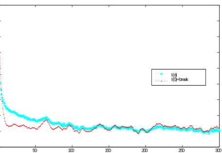
in Perron and Qu, 2004). Additionally, Figure 1 depicts, for T = 20;000, the estimated ACFs of two processes. The …rst one is a process like (1), with = 0:5 and ut being an
AR(1)process with a parameter equal to0:7;while the second one is an I(d) process with
d= 0:3. As can be inspected, except for the …rst few autocorrelations, the ACFs behave very similarly in both cases. Thus, this type of result illustrates the source of confusion which has been stressed in the literature. The problem aggravates even more when the DGP contains a break in the trend. For example, using the same experiment with a DGP given by yt = 1+ 1DT ( )t+"t , with DTt ( ) = (t TB)1(TB+1 t T); 1 = 0:1; and
"t n:i:d(0;1)yields estimates ofdin the range (1:008;1:0310), depending on the choice
of frequency, well in accord with the results of Perron (1989) about the lack of consistency of the DF test of a unit root in such a case.
1This result has been recently generalized by Mikosch and Starica (2004) to the case of multiple breaks in the mean.
0 50 100 150 200 250 300 -0.1 0 0.1 0.2 0.3 0.4 0.5 0.6 0.7 0.8 I(d) I(0)+break
Fig. 1. Sample ACF of an I(d) and an I(0)+break processes.
Table 1 GPH Estimates of d(DGP(1)) Frequency T0:5 T0:45 T0:4 T0:35 2 1 = 0:0 -0.004 -0.004 -0.003 -0.005 2 1 = 0:2 0.150 0.212 0.298 0.404 2 1 = 0:5 0.282 0.3709 0.477 0.585
Rejection of the null hypothesis d=0 at 1% signi…cance level (s.l.).
Along this way of reasoning, similar results about the possibility of confusing other types of nonlinear models withI(d)processes have been derived very recently in slightly di¤erent frameworks to the one discussed in (1). First, there is Parke’s (1999) error duration (ED) model, which considers the cumulation of a sequence of shocks that switch to 0 after a random delay that follows a power law distribution, so that if the delays were of in…nite extent the process would be a random walk, and if of zero extent, an i:i:d: process. Con-trolling the probability that a shock survives for k periods, pk, to decrease with k at the
rate pk = s2d 2 for d 2 (0;1]; Parke shows that the ED model generates a process with the same autocovariance structure as an I(d) process, i.e., y(j) = O(T2d 1) for large j. Secondly, there are Granger and Hyung ’s (1999) and Diebold and Inoue’s (2001) models which consider processes that are stationary and short memory, but exhibit periodic regime shifts, i.e., random changes in the mean of the series. For example, consider a DGP with
yt=mt+"tand mt=qt t;where = (1 L), and such thatqtfollows ani:i:d:binomial
distribution whereqt= 1with probabilitypand qt= 0with probability(1 p), and"t and
t are independent i:i:d: processes. Then, by assuming that the regime-shift probability p declines at a certain rate as the sample size increases, i.e., p=O(T2d 2);it can be shown that the variance of the partial sums in this model will be related to the sample size in just the same way as in anI(d)process, i.e., increasing at the rateT1+2d. Therefore, the message to be drawn from all these works is that modelers face a hazard of mis-identi…cation when the incidence of structural shifts is linked to the sample size in a particularad hoc way.
On the whole, the class of models described above are nonlinear models capable of re-producing some observationally equivalent characteristics ofI(d) processes, albeitnot all.2 Moreover, they do so as long as the incidence of the shifts is related to the sample size in the speci…c fashion described earlier, which may be too restrictive in practice. For this reason, we consider more relevant for practitioners to develop a test statistic which helps to distinguish an I(d) process from a short-memory process subject to a small number of breaks, in the spirit of DGP (1). Since among the I(0) processes subject to breaks, the ones having more impact on empirical research are those popularized by Perron (1989), which are tested againstI(1)processes as the null, our main contribution in this paper is to extend Perron’s testing approach to the more general setting ofI(d)processes, withd2(0; 1], instead of d= 1. For the most part, our analysis in the sequel will focus on the case of a single break, although we brie‡y conjecture about how to deal with processes containing more breaks.
In parallel with Perron (1989) who uses suitably modi…ed Dickey-Fuller (DF) tests for 2Davidson and Sibbersten (2003) have recently demonstrated that the normalized sequence partial sums offytggenerated by the ED and the other periodic regime shift models do not converge to fBM.
the I(1) vs. I(0) case in the presence of regime shifts, our strategy lies upon generalizing the Fractional Dickey-Fuller (FDF) approach proposed by Dolado, Gonzalo and Mayoral (DGM, 2002, 2004) to test I(1) vs. I(d), 0 d < 1; but now suitably modi…ed to test
I(d) vs. I(0) cum structural breaks: In DGM (2002) it was shown that if the order of fractional integration under the alternative is 0 d <1 and no deterministic components are present, then an unbalanced OLS regression of the form yt = dyt 1+"t, yields a consistent test of H0 : d = 1 against H1 : d 2 [0; 1) based on the t-ratio of bols in the previous regression model.3 If the error term in the DGP is autocorrelated, then the regression should be augmented with a suitable number of lagged values of yt:The degree of integration under the alternative hypothesis (d1) can be taken to be known (in a simple alternative) or estimated with a T12-consistent estimator (in a composite alternative).4 If
deterministic components, (t);are present under the null (say, a constant or a linear trend), DGM (2004) derive a FDF test now based on the regression yt=H(L) (t)+ dyt 1+"t, whereH(L) = dL:
Despite focusing on the test of I(1) vs. I(d) processes, DGM (2002) show that their results could be generalized to the case where the degrees of fractional integration under the null(d0)and the alternative(d1) verify the inequalityd1< d0:Accordingly, we propose in this paper a new test of I(d) vs. I(0) cum structural breaks, namely d0 = d 2 (0;
0:5)[(0:5;1]5 andd1= 0;along the lines of the well-known procedures proposed by Perron (1989) when the date of the break is taken to be a priori known, and the extensions of Banerjee et al. (1992) and Zivot and Andrews (1992) when it is assumed to be unknown.
3
To operationalise the FDF test , the regressor dyt 1is constructed by applying the truncated binomial
expansion of the …lter(1 L)dtoyt, so that dyt =Pt01 i(d)yt i;where i(d)is the i-th coe¢ cient in
that expansion given by i= (i d)= ( d) (i+ 1)with (:)the Gamma function.
4Empirical applications of such a testing procedure can be found in DGM (2003), whereas a generalization of the FDF test in theI(1)vs. I(d)case allowing for deterministic components (drift/ linear trend) under the maintained hypothesis has been developed in DGM (2004).
5Although the case of d = 0:5was treated in DGM (2002), it constitutes a discontinuity point in the analysis ofI(d)processes; cf. Liu (1998). For this reason, as is often the case in the literature, we exclude this possibility in our analysis. Nonetheless, to simplify notation in the sequel, we will refer to the permissable range ofdunder the null as0< d 1:
To avoid confusion with the FDF for unit roots, the test presented hereafter will be denoted as theStructural Break FDF test (SB-FDF henceforth). It is based on the t-ratio ofbolsin an OLS regression of the form d0y
t = (L)AB(t) + yt 1+"t, where (L) = d L
and AB(t) captures di¤erent structural breaks. As in Perron (1989), we will consider the following possibilities: a crash shift, a changing growth shift, and a combination of both.6
At this stage it should be stressed that a test that extends Perron’s DF testing approach ofI(1)vs. I(0)cum structural breaks to a null ofI(d) withd2(0;1]can be very useful in order to improve the power of the DF test when the true process isI(d) butd <1. In such an instance, Sowell (1990) and Krämer (1998) have shown that the DF and ADF tests are consistent, i.e. they reject the null of I(1) with probability one as the sample size tends to in…nity. However, the simulation results in Diebold and Rudebusch (1991) indicate that the power against fractional alternatives in …nite samples can be low in some cases . To obtain further evidence on this issue, we report in Table 2 the rejection frequencies of Zivot and Andrews (1992) generalization of Perron’s (1989) DF test in the case where the true DGP is an I(d) process with 0< d <1; and I(1)is tested against I(0) cum a changing growth shift, assuming thatTB is unknown. The number of replications is5;000and "t n:i:d(0;
1). As can be observed, whenT = 100;the rejection frequencies of the I(1) null hypothesis are high for values of dup to 0:7 but then, as one would expect, falls drastically asd gets closer to unity:For T = 400, this reduction in power occurs when d is above 0:8. In light of our previous discussion about the confound of LRD and structural breaks, these results seem to imply that, when the true series is I(d), for low and moderate values of d, one is bound to …nd structural breaks “too often”, whereas for high values of d; the false null of
I(1) will hardly be rejected. Thus, this evidence supports the need of a test where the null 6Note, however, that extensions to more than one break, along the lines of Bai and Perron (1998) and Bai (1999) should not be too di¢ cult to devise once the simple case of a single break is is worked out. Some discussion on this case can be found in Section 4.
isI(d).
TABLE 2
Power of DF test of I(1) vs. I(0)+breaks
Regression Model: yt= + t+ DTt (0:5) + yt 1+"t DGP: d0y t="t;"t n:i:d(0;1) Sample size/d0 0.1 0.2 0.3 0.4 0.5 0.6 0.7 0.8 0.9 T=100 100% 100% 99.9% 99.7% 94.4% 73.0% 38.0% 14.2% 4.0% T=400 100% 100% 100% 100% 100% 99.9% 93.5% 49.9% 8.9% Lastly, to place our SB-FDF test in the existing literature, it is convenient to di¤erentiate between several characterizations of the process governing the evolution of a time series under the null and alternative hypotheses. These di¤erent characterizations depend upon the degree of integration of the series and the potential existence of structural breaks in its deterministic components. Speci…cally, four possibilities can be considered: (I)I(0)and no structural breaks; (II) I(0) and structural breaks; (III)I(d) and no structural breaks, and (IV)I(d) and structural breaks. The cases (I) against (II), and (I) against (III) have been extensively analyzed in the literature; cf. for the former see Perron (2005), and for the latter see Robinson (2003). The case (III) against (IV), when 0< d <0:5, has also been treated, among others, by Hidalgo and Robinson (1996) when the break date is assumed to be known, and by Lazarova (2003) who extends their analysis to the case where the break date is considered to be unknown. Using a frequency-domain approach, Hidalgo and Robinson (1996) derive a test statistic whose limiting distribution under the null of no break is chi-squared for the former case, whereas in the case of an unknown break critical values need to be obtained by bootstrap methods (see Lazarova, 2003). Sibbertsen and Venetis (2004) have also studied the case where there are only shifts in mean, the break date is considered to be unknown, and0< d <0:5:Their test is based upon the (squared) di¤erence between the GPH estimator of d and its tapered version, which converges to zero under the null of no break and diverges under the alternative of a break. It has a limiting chi-squared distribution if the errors are gaussian; otherwise, again bootstrap methods need to be used
to obtain critical values. The case (II) versus (IV) has been treated by Giraitis, Kokoszka and Leipus (2001) who analyze how large the size of the mean shift in an I(0) series has to be in order to be mistaken with a stationary long-memory process (0< d <0:5)in a given sample.
In comparison to all these previous works, the case considered in this paper is (III) against (II) which surprisingly has received much less attention in the literature. This is the case that can really help in solving the identi…cation issue between LRD and SB which can be extremely relevant for at least three reasons: (i) shock identi…cation (persistent vs. transitory), (ii) forecasting (do we need a long-history of the time series or only a short past will be of much use in forecasting?), and (iii) detection of spurious fractional cointegration (see Gonzalo and Lee, 1998). Indeed, Giraitis, Kokoszka and Leipus (2001) and the comments by Robinson to Lobato and Savin (1998) have stressed the importance of constructing a proper test statistic to distinguish between these alternative speci…cations. However, so far, the only attempt in this direction that we know of is Mayoral (2004a) whose approach relies upon a LR test in the time domain, but which is can only be applied to non-stationary processes under the null. Thus, to the best of our knowledge, there is not yet any available test in the literature for testing I(d) versus I(0) cum structural breaks allowing for both stationary and non-stationary processes under the null-hypothesis. This is the goal of the proposed SB-FDF test, which additionally presents the advantage of not requiring a correct speci…cation of a parametric model and other distributional assumptions, besides being computationally simple since it is based on an OLS regression.
The rest of the paper is organized as follows. In Section 2 we derive the properties of the FDF test forI(d) vs. I(0) in the presence of deterministic components, like a constant or a linear trend, but without considering breaks yet, to next discuss the e¤ects on this test of ignoring structural breaks in means or slopes when they exist.7 Given that, as discussed above, the power of this test can be severely a¤ected by parameter changes in
7
Note that the FDF tests proposed in DGM (2002, 2004) refer to the case of I(1)vs. I(d). Thus, this section extends our previous results to the new setup ofI(d)vs. I(0);withd2(0;1].
the deterministic component of the process, the SB-FDF test of I(d) vsI(0)with a single structural break at a known or an unknown date is introduced in Section 3, where both its limiting and …nite-sample properties are analyzed in detail. Section 4 contains a brief discussion of how to modify the test to account for autocorrelated disturbances, in the spirit of the ADF test, leading to the SB-AFDF test (where “A” stands for augmented versions of the test-statistics) and conjectures on how to generalize the testing strategy to multiple breaks, rather than a single one. Section 5 contains two empirical applications; the …rst application deals with long U.S GNP series, where the stochastic or deterministic nature of their trending components has engendered some controversy in the literature; the second application centers on the behavior of the absolute values and squares of …nancial log-returns series, which has also been subject to some dispute. Finally, Section 6 concludes. Appendix A gathers the proofs of theorems and lemmae while Appendix B contains the tables of critical values for the cases where the limiting distributions are non-standard.
2. THE FDF TEST FOR I(D) VS. I(0)
2.1 Preliminaries
Before considering the case of structural breaks, it is convenient to start by analyzing the problem of testingI(d);with0< d 1, against trend stationarity, i.e. d= 0;along the lines of the FDF framework for the general case of I(d0) vs. I(d1) processes. The motivation for doing this is twofold. First, taking an I(d) process as a generalization of the unit root parameterization, the question of whether the trend is better represented as a stochastic or a deterministic component arises on the same grounds as in the I(1) case. And, secondly, the analysis in this subsection will provide the foundation for the treatment of the general case where non-stationarity can arise due to the presence of structural breaks.
Under the alternative hypothesis,H1;we consider processes with an unknown mean or a linear trend ( + t);
yt= +
"t1(t>0)
yt= + t+
"t1(t>0)
d0 L; (5)
where, "t is assumed to be i:i:d.(0, 2" ), with0 < 2 <1;and d0 2(0;1]:Hence, under
H1;
d0y
t= + d0 + yt 1+"t; (6)
d0y
t= + d0 + t+ d0 1'+ yt 1+"t; (7)
where = , = ; = and'= :For simplicity, hereafter we write"t1(t>0)="t. Under H0; when = 0; d0yt = d0 +"t in (6) and d0yt = d0 + d0 1 +"t in (7).8 Thus, E( dyt) = d and E( dyt) = d( + t), respectively. Note that d =
Pt 1
i=0 i(d) and d 1 =
Pt 1
i=0 i(d 1) where the sequence f i( )g1i=0 comes from the expansion of (1 L) in powers of L and the coe¢ cients are de…ned as i( ) = (i
)=[ ( ) (i+ 1)]:In the sequel, we use the notation t( ) =Pti=11 i( ):Also note that
t(d) for d < 0 induces a deterministic trend which is less steep than a linear trend and
coincides with it whend= 1since t( 1) =Pti=01 i( 1) =t: As demonstrated in DGM (2004), (:) is a concave function for values of d < 0, being the function less steep the smaller (in absolute value) d is. Under H1; the polynomial (z) = (1 z)d z has absolutely summable coe¢ cients and veri…es (0) = 1 and (1) = 6= 0:All the roots of the polynomial are outside the unit circle if 2d< <0. As in the DF framework, this condition excludes explosive processes. Consequently, under H1; yt is I(0) and admits the representation
yt = +ut; oryt= + t+ut;
ut = (L)"t; (L) = (L) 1:
Computing the trends t( ); = d ord 1 in (6) or (7) does not entail any di¢ culty since it only depends ond0;which is known underH0. As discussed earlier, the case where
8
d0 = 1 and a linear trend is allowed under the alternative of d1 =d; 0 < d <1; has been analyzed in DGM (2004) where it is shown that the FDF test is (numerically) invariant to the values of and in the DGP.
Next, we derive the corresponding result for H0 :d0 =d; d2(0;1]vs. H1 :d1 = 0:The following theorem summarizes the main result:
Theorem 1 Under the null hypothesis that yt is an I(d) process de…ned as in (4) or (5)
with = 0;the OLS coe¢ cient associated to in regression model (6); ^ols; or (7); ^ols;
respectively is a consistent estimator of = 0 and converges at a rate Td if 0:5 < d 1 and at the usual rateT1=2 when0< d <0:5. The asymptotic distribution of the associated
t statistic, ti ^ ols ; i={ ; g is given by ti^ ols w ! R1 0 B i d(r)dB(r) R1 0 Bdi(r) 2 d(r) 1=2 ; if0:5< d 1, and ti^ ols w !N(0;1); if 0< d <0:5;
where !w denotes weak convergence and Bdi(r) withi={ ; g is the L2 projection residual from the continuous time regressions9 Bd(r) = ^0 + ^2r d+Bd(r) and Bd(r) = ^0 +
^1r d+ ^2r1 d+ ^3r+Bd(r);respectively.
The intuition for this result is similar to the one o¤ered by DGM (2002) in the case of
I(1) vs. I(d) processes with 0 < d < 1. The di¤erent nature of the limiting distributions depend on the distance between d0 and d1: When d0 (= 1 in the DGM case ) andd1 are close, then the asymptotic distribution is asymptotically normal whereas it is a functional of fBM when both parameters are far apart. Hence, since in our case d0 = d; 0 < d 1; and d1 = 0; asymptotic normality arises when 0 < d <0:5: Also note that d0 = 1 renders the standard DF limiting distribution.
9The parameters ^0; ^1; ^2; and ^3 solve min 0; 1 R1 0 Bd(r) ^0 ^1r d2dr and min 0; 1; 2; 3 R1 0 Bd(r) ^0 ^1r d
+ ^2r1 d+ ^3r 2dr for the constant and constant and trend cases, respectively:
The …nite-sample critical values of the cases considered in Theorem 1 are presented in Appendix B (Tables B1 and B2). Three sample sizes are considered, T = 100; 400 and
1;000, and the number of replications is10;000. Table B1 gathers the corresponding critical values for the case where the DGP is a pure I(d) without drift (since the test is invariant to the value of ); i.e, dyt ="t with "t n:i:d (0; 1); when (6) is considered to be the regression model. Table B2, in turn, o¤ers the corresponding critical values when (7) is taken to be the regression model. As can be observed, the empirical critical values are close to those of a standardized N(0;1) (whose critical values for the three signi…cance levels reported below are 1:28, 1:64 and 2:33, respectively, ) when 0< d <0:5;particularly forT 400:However, ford >0:5the critical values start to di¤er drastically from those of a normal distribution, increasing in absolute value asdgets larger.
As for power, Table 3 reports the rejection rates at the 5% level (using the e¤ective sizes in Table B2) of the FDF test in (7) in a similar Monte Carlo experiment to the one above, where now the DGP is an i.i.d. process cum a linear trend, i.e., yt = + t+"t, with
= 0:1; = 0:5:The main …nding is that, except for low values of dand T = 100where rejection rates of the null still reach 55%, the test turns out to be very powerful in all the other cases.
TABLE 3
Power (Corrected size: 5%)
Regression Model: d0y t= + t(d) + t+' t(d 1) + yt 1+"t DGP: yt= + t+"t; = 0:1; = 0:5; "t n:i:d (0;1) d0/ Sample size T = 100 T = 400 T = 1000 0.2 54.9% 98.9% 100% 0.4 98.4% 100% 100% 0.7 100% 100% 100% 0.9 100% 100% 100% 1.0 100% 100% 100%
2.2 The e¤ects of structural breaks on the FDF test of I(d) vs. I(0)
Following Perron’s (1989) analysis in his Theorem 1, our next step is to assess the e¤ects on the FDF tests forI(d)vs. I(0)of ignoring the presence in the DGP of a shift in the mean of the series or a shift in the slope of the linear trend. Let us …rst consider the consequences of performing the FDF test with an invariant mean, as the one discussed above, when the DGP contains a break in the mean. Thus,yt is assumed to be generated by,
DGP 1: yt= 0+ 0DUt( ) +"t; (8)
where "t iid(0; 2") and DUt( ) = 1(TB+1 t T): Ignoring the break in the mean, the
SB-FDF test will be based on regression (6) which is repeated for convenience
dy
t= + t(d) + yt 1+"t: (9)
Then, the following theory holds.
Theorem 2 If yt is given by DGP 1 in (8) and regression model (9)is used to estimate ;
when TB = T for all T and0< <1;then, as T ! 1;it follows that,
^ ols p ! d 2 "[C12(d) C2(d)] D(d; 2 ") ; if 0 < d <0:5, ^ ols p ! d 2 [ 20 (1 ) + 2 "] ; if 0:5 < d 1; and, t^ ols p ! 1; if 0< d 1;
where !p denotes convergence in probability,
D d; 2" =C12(d) [ 0 (1 ) + 2"] C2f 20(2 1 d) 2 1 d 1 + 2"g;
and
Theorem 2 shows that, under the crash hypothesis, the limit depends on the size of relative shift in the mean, 0: Note that if = 0 or = 1; i.e., when there is no break, then bols !p d: This result is quite intuitive since, being yt I(0) under DGP 1; the covariance between dytand yt 1 is 1(d) = d:Further, for d= 1, the expression in part (a) in Theorem 1 of Perron (1989) is recovered, generalizing therefore his results to the more general case ofd2(0;1]. Moreover, the fact thatbols converges to a …nite negative number implies that T1=2bols ford2(0;0:5); Tdbols ford2(0:5;1)and the corresponding t-ratios in each case will diverge to 1. Thus the FDF test for I(d) vs. I(0) would eventually reject the null hypothesis of d = d0, 0 < d0 < 1; when it happens to be false. Notice, however, that, as in Perron’s analysis, the power of the FDF test will be decreasing in the distance between the null and the alternative, namely asdgets closer to its true zero value, and in the size of the break, namely as 0 gets larger relative to 2".
Next consider the case where there is a (continuous) break in the slope of the linear trend, such thatyt is generated by,
DGP 2: yt= 0+ 0t+ 0DTt( ) +"t; (10)
where DTt ( ) = (t TB)1(TB+1 t T). The FDF test is again implemented ignoring the
breaking trend, that is, it is computed in the regression,
dy
t= + t+ t(d) +' t(d 1) + yt 1+"t: (11)
Theorem 3 If yt is given by DGP 2 in (10) and regression model(11) is used to estimate
;when TB= T for allT and 0< <1; then, as T ! 1;it follows that
tb ols p !+1 if 0< d <0:5; and, tb ols p !0; if 0:5< d 1:
In contrast to the result in Theorem 2, the FDF is unambiguously inconsistent when a breaking trend is ignored. The intuition behind this result, which again extends part (b)
of Theorem 1 in Perron (1989) to our more general setting, is that bols is Op(T d) with a positive limiting constant term for d 2(0; 1] and that the sample s.d (bols) is Op(T 1=2), implying that the t-ratio isOp(T1=2 d):Therefore, it will tend to 0;ford2(0:5;1];and to
+1;ford2(0;0:5).
In sum, the FDF test for I(d) vs. I(0) without consideration of structural shifts is not consistent against breaking trends and, despite being consistent against a break in the mean, its power is likely to be reduced if such a break is large. Hence, there is a need for alternative forms of the FDF test that could distinguish an I(d) process from a process beingI(0)around deterministic terms subject to structural breaks.
3. THE SB-FDF TEST OF I(D) VS. I(0) WITH STRUCTURAL BREAKS
Given the above considerations, we now proceed to derive the SB-FDF invariant test for
I(d) vs. I(0) allowing for structural breaks underH1:To account for structural breaks, we consider the following variant of (5) as the maintained hypothesis,
yt=AB(t) +
at1(t >0)
d L ; (12)
where AB(t) is a linear deterministic trend function that may contain breaks at unknown dates (in principle, just a single break at dateTBwould be considered) andatis a stationary
I(0)process. In line with Perron (1989) and Zivot and Andrews (1992), the null hypothesis of I(d) will be implied by a value of = 0 whereas <0 means that the process is I(0):
In line with these papers, three de…nitions ofAB(t)are considered,
Case A: AAB(t) = 0+ ( 1 0)DUt( ); (13)
Case B: ABB(t) = 0+ 0t+ ( 1 0)DTt ( ); (14)
Case A corresponds to the crash hypothesis, case B to the changing growth hypothesis and case C to a combination of both. The dummy variablesDUt( )andDTt ( )are de…ned as before, and DTt( ) =t1(TB+1 t T) with =TB=T:
Initially, let us assume that the break date TB is known a priori and thatat="t where
"t is an i:i:d(0; 2) process. Then, the SB-FDF test of I(d) vs. I(0) in the presence of
structural breaks is based on the t-ratio of the coe¢ cient in the regression model,
dy
t= dAiB(t) AiB(t 1) + yt 1+"t; i=A; B; and C: (16)
As above, the SB-FDF test is invariant to the values of 0; 1; 0 and 1under H0: Following the discussion in section 2.1, it is easy to check that under H1 : <0; yt is I(0) and is subject to the regime shifts de…ned by AiB(t). Conversely, under H0 : = 0, the process is I(d) with E[ d(yt AiB(t))] = 0:Using similar arguments to those employed in Theorem 1, the following theory holds.
Theorem 4 Let yt be a process generated as in (12) with at = "t i:i:d 0; 2 . Then,
when TB = T for all T and 0 < < 1; under the null hypothesis of = 0; the OLS
estimator associated to in regression model(16);asT ! 1;is consistent. The asymptotic distribution of the associated t ratio is given by,
tib ( ) w ! R1 0 B i d ( ; r)dB(r) R1 0 Bdi( ; r) 2d(r) 1=2 ifd 2 (0:5;1]; tib ( ) w !N(0;1) ifd 2 (0;0:5);
where Bdi(:; :) is the L2 projection residual from the corresponding continuous time regres-sions associated to modelsi=fA; B; and Cg; de…ned in Appendix A.
Although it was previously assumed that the date of the break TB is known, in general this might not be the case. Thus, we explore in what follows how to implement the SB-FDF test under this more realistic situation.
For that, we follow the approach in Banerjee et al. (1992) and Zivot and Andrews (1992) by assuming that, underH0;no break occurs, that is, = 0; 0 = 1 and 0= 1;implying
that(12) can be written as, d(y t 0) =at; if i=A,t= 1; 2; :::; (17) or, d(y t 0 0t) =at; if i=fB and Cg; t= 1; 2; :::; (18)
where at is an I(0) process. As discussed before, under the alternative hypothesis, the process is I(0) and may contain a single break in (some of) the parameters associated to the deterministic components, that occurs at an unknown time TB = T; 2 (0; 1): Then, the potential break point under H1 will be estimated in such a way that gives the highest weight to the I(0) alternative. The estimation strategy will therefore consist in choosing the break point that gives the least favorable result for the null hypothesis ofI(d)
using the SB-FDF test in (16) for each of the three cases,i=A; B;andC. Thet statistic
on^iols, tb( );is computed for the values of 2 = (0:15;0:85), following Andrews’(1993) choice of range, and then the in…mum (most negative) value would be chosen to run the test. Thus, the test would reject the null hypothesis when
inf
2 tb( ) > k i
inf; ;
where kinfi ; is a critical value to be provided in Appendix B. Under these conditions, the following theory holds.
Theorem 5 Let ytbe a process generated as in(17)or(18)withat "t i:i:d 0; 2 and
possibly 0 = 0 = 0: Let be a closed subset of (0; 1). Then, under the null hypothesis of = 0;the asymptotic distribution of the t statistic associated to in regression model
(16), (with AAB(t) if yt is generated by (17) and ABB(t) or ACB(t) if yt is generated in (18))
is given by, inf 2 t i b( ) w ! inf 2 R1 0 Bdi( ; r)dB(r) R1 0 B i d ( ; r) 2d(r) 1=2 if d2(0:5;1]; i=fA; B and Cg and, inf 2 t i b( ) w !N(0;1) if d2(0; 0:5):
To compute critical values of the inf SB-FDF t-ratio test, a pure I(d0) process with
"t n:i:d:(0;1)has been simulated 10;000times, whereas the three regression models (A,
B; and C) have been considered for samples of size T = 100; 400; 1000. Notice hat the sequence ftib
( )g are normally distributed and perfectly correlated. Hence, as shown in the proof of Theorem 5, the inf of this sequence corresponds to a N(0, 1) as well. However, in …nite samples, there are several asymptotically negligible terms which depend on the product (1 ) 1T 2 ; 0 < < 1; which may be sizeable for su¢ ciently large (small) values of ( ) at a given T (see equation A.2 in the Appendix). Tables B3, B4 and B5 in Appendix B report the corresponding critical values which, due to the presence of those terms, are larger (in absolute value) than the critical values of the SB-FDF test reported in Tables B1 and B2 when considering the left tail. Even for T = 1000, the critical values for d 2 (0; 0:5) are to the left of those of a N(0;1) and, in unreported simulations, we found that they slowly converge to them for sample sizes with around 5000 observations. Thus, for smaller sample sizes, we advice to use the e¤ective critical values rather than the nominal ones.
In order to examine the power of the test, we have generated 5000replications of DGP 2 (10) with sample sizes T = 100 and 400, where = 0:5, i.e., a changing growth model with a break in the middle of the sample. Both regression models B and C , in (16), have been estimated. Rejection rates are reported in Table 4 where, in order to compute the size-corrected power, the corresponding critical values in Tables B4 and B5 have been used. The power is very high except whend= 0:1and T = 100but even in this case it is close to 50% whenT = 400.10
1 0
In DGM (2002, 2004), we provide both Monte-Carlo and analytical results showing that the FDF test for I(1)vs. I(d) processes has better size-corrected power, except for very local alternatives (and even in this case the loss in power is small), than other available time-domain tests in the literature, like Tanaka’ s (1999) LM test. Unreported calculations (available upon request), show that this is also the case for our newI(d)vs. I(0)testing setup.
TABLE 4
Power inf SB-FDF, I(d) vs. I(0) + S.B.
Regression Model: dy
t= dAiB(t) AiB(t 1) + yt 1+"t; i=fB; Cg
dgp: yt= 0+ 0t+ 0DTt( ) +"t; 0= 1; 0= 0:5; = 0:5; "t n:i:d(0;1)
0 = 0:1 0 = 0:2
RModel B RModel C RModel B RModel C
d0=Sample size T=100 T=400 T=100 T=400 T=100 T=400 T=100 T=400 0.1 15.6% 50.3% 14.5% 48.9% 13.7% 48.9% 12.4% 47.4% 0.3 67.4% 74.9% 26.2% 73.5% 66.3% 73.4% 62.9% 71.3% 0.6 99.7% 100% 68.8% 100% 99.8% 100% 99.6% 100% 0.7 100% 100% 98.0% 100% 100% 100% 100% 100% 0.9 100% 100% 99.9% 100% 100% 100% 100% 100%
4. AUGMENTED SB-FDF TEST AND MULTIPLE BREAKS
The limiting distributions derived above are valid for the case where the innovations
are i:i:d: and no extra terms are added in the regression equations. If some
autocorre-lation structure are allowed in the innovation process, then the asymptotic distributions will depend on some nuisance parameters. To solve the nuisance-parameter dependency, two approaches have been typically employed in the literature. One is the non-parametric approach proposed by Phillips and Perron (1988) which is based on …nding consistent es-timators for the nuisance parameters. The other, which is the one we follow here, is the well-known parametric approach proposed by Dickey and Fuller (1981) which consists of adding a suitable number of lags of dyt to the set of regressors (see DGM; 2002): As Zivot and Andrews (1992) point out, a formal proof of the limiting distributions when the assumption ofi:i:d:disturbances is relaxed is likely to be very involved. However, along the lines of the proof for the AFDF test in Theorem 7 of DGM (2002), it can be conjectured that if the DGP is dyt=ut1(t>0) and ut follows an invertible and stationary ARMA(p; q)
process p(L)ut = q(L)"t with Ej"tj4+ <1 for some >0;then the inf SB-FDF test based on the t-ratio of bols in (19) augmented with k lags of dyt will have the same lim-iting distributions as in Theorem 5 above and will be consistent whenT ! 1and k! 1, as long as k3=T ! 0:Hence, the augmented SB-FDF test (denoted as SB-AFDF) will be based on the regression model,
dy t= dAiB(t) AiB(t 1) + yt 1+ k X j=1 &j dyt j+at; i=A; B; andC: (19)
Although a generalization of the previous results to multiple breaks is not considered in this paper, it is likely that this extension can be done following the same reasoning as in the procedure devised by Bai and Perron (1998). In their framework, where there are m possible breaks a¤ecting the mean and the trend slope, they suggest the following procedure to select the number of breaks. Letting sup FT(l) be the F- statistic of no structural break(l= 0)vs. kbreaks (k m);they consider two statistics to test the null of no breaks against an unknown number of breaks given some speci…c bound on the maximum number of shifts considered. The …rst one is the double maximum statistic (UDmax)where UDmax= max1 k msupFT(l) while the second one is supFt(l+ 1=l) which test the null of
l breaks against the alternative ofl+ 1 breaks. In practice, they advise to use a sequential procedure based upon testing …rst for one break and if rejected for a second one, etc., using the sequence ofsupFt(l+ 1=l)statistics. Therefore, our proposal is to use such a procedure to determine 1; :::; k in the AB(t) terms in (16). By continuity of the sup function and tightness of the probability measures associated withtb
ols, we conjecture that a similar
result to that obtained in Theorem 5 would hold as well, this time with thesupof a suitable functional of fBM. Derivation of these results and computation of the corresponding critical values exceeds the scope of this paper but they are in our future research agenda.
5. EMPIRICAL APPLICATIONS
In order to provide some empirical illustrations of how easy the SB-FDF test can be used in practice, we consider the following two applications.
5.1 Real GNP.—
The …rst application deals with the log. of a long series of U.S. real GNP, yt;which basi-cally corresponds to the same data set used in Diebold and Senhadji (1996) (DS henceforth) in their discussion on whether GNP data is informative enough to distinguish between trend stationarity (T-ST) and …rst-di¤erence stationarity (D-ST). The data are annual and range from 1869 to 2001 giving rise to a sample of 133 observations where the last 8 observations have been added to DS´s original sample ending in 1995; cf. Mayoral (2004b), for a detailed discussion of the construction of the series. Since this series is based on the historical annual real GNP series constructed by Balke and Gordon (1989), it is denoted as GNP-BG.11
According to DS’s analysis, there is conclusive evidence in favor of T-ST and against D-ST. To achieve this conclusion, DS follow Rudebusch (1993)’s bootstrap approach in computing the best-…tting T-ST and D-ST models for the series. Then, they compute the exact …nite sample distribution of the t-ratios of the lagged (log. of) GNP-BG level in an augmented Dickey-Fuller (ADF) test for a unit root when the best-…tting T-ST D-ST models are used as the DGPs. Their main …nding is that the p-value of the ADF test is very small under the D-ST model but quite large under the T-ST model, providing overwhelming support in favour of the latter model. Nonetheless, as DS acknowledge, rejecting the null does not mean that the alternative is a good characterization of the data. Indeed, Mayoral (2004b) has pointed out that when the same exercise is done with the well-known KPSS test, where the null is TS-T, it is also rejected in both series. This inconclusive outcome leads this author to conjecture that, since both the I(0) and I(1) null hypotheses are rejected, it may be the case that the right process is an I(d), 0 < d < 1: Considering values of d
in the range 0.6-0.7, she …nds favorable evidence for an I(d) using the FDF test of I(1)
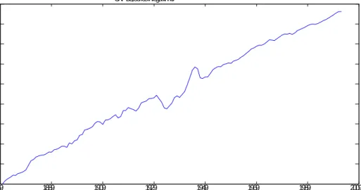
vs. I(d), which rejects the null, and a LR test of I(d) vs. I(0);which does not reject the null. Nonetheless, from inspection of Figure 2, where the log. of GNP-BG is displayed, one could as well conjecture that the data are generated by a T-ST process subject to some
1 1
Following DS (1996), we have also implemented the SB-FDF test to a long series of U.S. real GNP based on the historical annual series of Romer (1989). The results, available upon request, are not reported since they are very similar to those displayed in Table 5.
1869 1889 1909 1929 1949 1969 1989 2009 4.5 5 5.5 6 6.5 7 7.5 8 8.5 9 GNP-BG, series in logarithms
Fig. 2. Plot of (logged) real GNP-BG series.
structural breaks as in Perron (1989). Hence, given the mixed evidence about the data being generated either by anI(d)process or by anI(0)processcum structural breaks, this example provides a good illustration of the usefulness of the SB-FDF test.
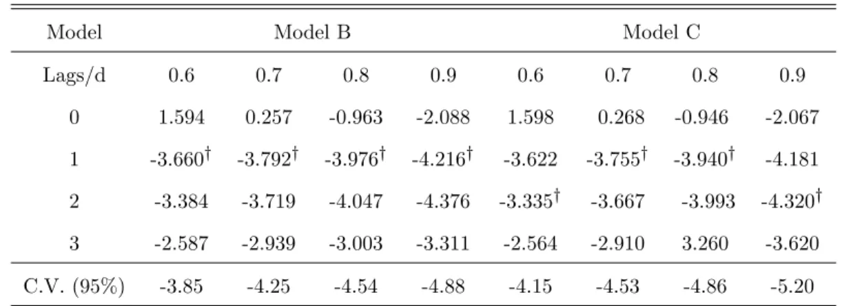
In Table 5, we report the t-ratios of the inf SB-AFDF test constructed according to (19) where up to three lags of dyt have been included as additional regressors in order to account for residual correlation. The critical values that have been employed are those reported in Tables B4, B5 for T = 100. Values of d in the non-stationary (albeit mean-reverting) range (0:5; 1) have been used to construct dyt and dAiB(t); i = B; and C, since the trending behaviour of the series precludes the use of model A which does not include a linear trend in the maintained hypothesis.
TABLE 5
inf SB-AFDF Tests
GNP-BG series
Model Model B Model C
Lags/d 0.6 0.7 0.8 0.9 0.6 0.7 0.8 0.9 0 1.594 0.257 -0.963 -2.088 1.598 0.268 -0.946 -2.067 1 -3.660y -3.792y -3.976y -4.216y -3.622 -3.755y -3.940y -4.181 2 -3.384 -3.719 -4.047 -4.376 -3.335y -3.667 -3.993 -4.320y 3 -2.587 -2.939 -3.003 -3.311 -2.564 -2.910 3.260 -3.620 C.V. (95%) -3.85 -4.25 -4.54 -4.88 -4.15 -4.53 -4.86 -5.20 ynumber of lags chosen by the AIC criterion. Rejection at the 95% s.l.
As can be inspected, the null of I(d) cannot be rejected at the conventional signi…cance level. Interestingly, this result against T-ST is reinforced by application of the conventional Zivot and Andrews’(1992) inf test for the null ofI(1), with two lags, which yields values of 4:23 (model B) and 5:03 (model C) against 5% critical values of 4:42 and 5:08;
respectively. However, concluding that the series is I(1) may not be correct (see Table 2), given the results of the SB-AFDF test which does not reject the null for large values of d, yet below unity.
In sum, the evidence provided by the SB-FDF test seems to point out that the GNP-BG series behaves as anI(d)process with a large d. This result is qualitatively consistent with other empirical investigations of fractional processes in GNP, such as Sowell (1992), on the basis that GNP is obtained by aggregating heterogeneously persistent sectorial value added which, according to Granger’s (1980) aggregation argument, yields long memory. In the same direction, recently Michelacci (2004) has shown that if Gibrat’s law fails and small …rms grow faster than big …rms, as empirical evidence suggests, aggregate output should exhibit a fractional order of integration.
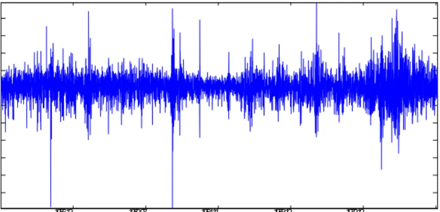
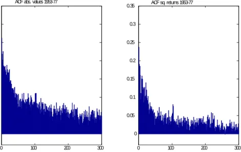
The second application deals with the (absolute values and squared) …nancial returns series, rt, obtained from the Standard & Poor’s 500 composite stock index over the period January 2, 1953 to October 10, 1977 (the number of observations is6217). This series has been modelled in several papers where it has been argued that shifts in the unconditional variance of an ARCH or GARCH model may induce the typical ACF of a long memory process (see, inter alia, Ding et al., 1996, Lobato and Savin (1998), and Mikosch and Starica, 2004). Notice that, although the sample considered in these papers are quite longer than ours, we restrict our sample to 1953-1977 because Mikosch and Starica (2004) claim that there is a single structural break in the constant term of a GARCH (1,1) model over that period, as a consequence of the …rst oil crisis in 1973.12 Since our proposed approach refers to a single shift, we deem this an appropriate choice of sample size. Further, the end of the sample has been chosen so that the potential break date in included in the range
2[0:15;0:85]used to implement theinf SB-AFDF test. From Figure 3, where the stock returns are depicted, it becomes clear that the series experiences a higher variance after 1973. Figures 4a and b shows the ACF for the absolutes values, jrtj;and the squares, r2t; respectively, which display the typical plateau for longer lags, as if LRD were present. The results of performing the inf SB-AFDF test for an unknown break date in version A ( no trend) of model (19) are shown in Table 6, where the number of lags is k = 15 (further lags were insigni…cant), and only values of d < 0:5 have been used, in agreement with the estimates of d obtained from the estimation of ARFIMA models applied to both series. Since the sample size in this case is large enough to use the N(0, 1) approximation for the limiting distribution, a 5% critical value of -1.64 is used. The main …nding is that the null hypothesis ofI(d)cannot be rejected for moderate values ofd, in the range0:1 0:4forjrtj, and0:1 0:3forr2
t, which contain the estimated values ofdfor this data set.13 Note that in the case of jrtj, the null of d= 0:4could be almost rejected at the 10% level (with a c.v. of
1 2For example, the estimates of the GARCH (1,1) model 2
t = 0+ 1 2t 1+ 1h 2
t 1yield 0=:325x10 6; 1= 0:150; 1= 0:600for T=1953-1972 and 0=:1:40x10 5; 1= 0:150; 1= 0:600for T=1953-1977.
1 3
The estimated values ofdusing the GPH approach with g(T) =T0:5;aredb= 0:4005for the absolute values, anddb= 0:3241for the squares of the returns.
1956.12 1960.07 1964.11 1968.12 1972.12 . -0.06 -0.05 -0.04 -0.03 -0.02 -0.01 0 0.01 0.02 0.03 0.04 Log returns 1953-1957
Fig. 3. Plot of S&P 500 daily returns, 1953-1977.
-1.28) whereas it is clearly rejected in the case ofrt2 at the 5% level.14 Hence, overall , the SB-AFDF test yields some evidence in favor of these transformation of the stock returns behaving during 1953-1977 asI(d)processes with a low degree of fractional integration. Of course, fractional integration and structural breaks can cohabit (for an empirical illustration see Choi and Zivot, 2005), yet its consideration is beyond the scope of this application.
TABLE 6
inf SB-AFDF tests S&P 500 data 1953-1977 d 0.1 0.2 0.3 0.4
jrtj 2:561 1:549 0:294 1:214
r2t 1.063 0.037 -1.216 -2.680
Rejection at the 95% s.l.;rt= logPt logPt 1:
1 4This conclusion is reinforced when we perform the test for the nonstationary null ofd= 0:6:With a 5% c.v. of -2.54 (see the left panel in Table B3), the values of the test for the absolute values and the squares are -4.63 and -6.15, respectively. Thus the null is strongly rejected.
0 100 200 300 0 0.05 0.1 0.15 0.2 0.25 0.3 0.35 0 100 200 300 0 0.05 0.1 0.15 0.2 0.25 0.3 0.35
ACF abs. values 1953-77 ACF sq. returns 1953-77
lag lag
Fig. 4. Sample ACF abs. values and squares of S&P 500 returns.
6. CONCLUSIONS
One of the recent identi…cation issues in time series is the di¢ culty in distinguishing long-memory from structural breaks. This can be extremely relevant for at least three reasons: (i) shock identi…cation (persistent vs. transitory), (ii) forecasting (do we need a long-history of the time series or only a short past will be of much use in forecasting?), and (iii) detection of spurious fractional cointegration. In order to contribute to solve this empirical identi…cation problem, in this paper we provide a simple test of the null hypothesis of a process being I(d); d 2(0; 1] against the alternative of being I(0) with deterministic terms subject to structural changes at known or unknown dates. The test, denoted as Structural Break Fractional Dickey-Fuller (SB-FDF) test, is a time-domain one, performs fairly well in …nite samples in terms of power, and it is easy to implement since it relies on a time-series OLS regression. Denoting by AB(t) the di¤erent types of a single structural break considered by Perron (1989), the SB-FDF test is based on the t-ratio of the coe¢ cient on yt 1 in an OLS regression of dyt on dAB(t); AB(t 1)and yt 1:A suitable number
of lags of dytmay be added to account for serially correlated errors. Whend2(0:5;1]its asymptotic distribution is nonstandard and critical values are simulated. By contrast, when
d2(0;0:5), it is asymptotically normally distributed. In future research we plan to extend the proposed testing approach to multiple breaks along the lines discussed in Section 4 of this paper, as well as to test I(d0) versusI(d1)cum structural breaks with d0 > d1.
REFERENCES
Andrews, D. W. K. (1993): “Test for parameter instability and structural break with unknown change point,”Econometrica, 61, 139-165.
Bai, J.(1999): “Likelihood ratio tests for multiple structural changes,”Journal of Econo-metrics, 91, 299-323.
Bai, J. and P. Perron (1998): “Estimating and testing linear models with multiple structural changes,”Econometrica, 66, 47-78.
Baillie, R.T. (1996): “Long memory processes and fractional integration in economics and …nance,”Journal of Econometrics, 73, 15-131.
Balke, N. and R. J. Gordon (1989): “The estimation of prewar gross national prod-uct: methodology and new evidence,”Journal of Political Economy, 97, 38-92.
Banerjee, A., R. Lumsdaine and J. H. Stock (1992): “Recursive and sequential tests for a unit root and structural breaks in long annual GNP series,”Journal of Business and Economic Statistics, 10, 271-287.
Beran, J.(1994): Statistics for long memory processes. New York. Chapman and Hall.
Bhatacharya, R.N., Gupta, V.K., E. Waymire (1983): “The Hurst e¤ect under trends,”Journal of Applied Probability, 20, 649-662.
Brockwell, P.J. and R.A. Davis (1991): Introduction to time series and forecasting. Springer, New York.
Choi, K. and E. Zivot (2005): “Long memory and structural breaks in the forward discount: An empirical investigation,”Journal of International Money and Finance (forth-coming).
Davidson, J. (1994): Stochastic Limit Theory. New York: Oxford University Press.
Davidson, J. and P. Sibbertsen(2003): “Generating schemes for long memory processes: Regimes, Aggregation and Linearity,” University of Cardi¤ (mimeo).
Dickey, D. A. and W.A. Fuller (1981): “Likelihood ratio tests for autoregressive time series with a unit root,”Econometrica, 49, 1057-1072.
against fractional alternatives,”Economic Letters, 35, 155-160.
Diebold, F and A. Inoue (2001): “Long memory and regime switching,”Journal of Econometrics, 105, 131-159.
Diebold, F. and S. Senhadji (1996): “The uncertain unit root in Real GNP: Com-ment,”American Economic Review, 86, 1291-98.
Ding, Z. and C.W.J. Granger(1996): “Modelling volatility persistence of speculative returns: A new approach,”Journal of Econometrics, 73, 185-215.
Dolado,J. ,Gonzalo, J. and L.Mayoral (2002): “A fractional Dickey-Fuller test for unit roots,”Econometrica, 70, 1963-2006.
Dolado, J., Gonzalo, J. and L.Mayoral, (2003): “Long range dependence in Span-ish political poll series,”Journal of Applied Econometrics, Vol. 18, No. 2, 137-155.
Dolado,J. Gonzalo, J. and L. Mayoral, (2004): “Testing I(1) vs. I(d) alternatives in the presence of deterministic components,” Universidad Carlos III (mimeo).
Geweke, J. and S. Porter-Hudak (1983): “The estimation and application of long memory time series models,”Journal of Time Series Analysis, 4, 15-39.
Giraitis, L., Kokoszka, P. and Leipus, R. (2001): “Testing for long memory in the presence of a general trend,”Journal of Applied Probability, 38, 1033-1054.
Gonzalo, J. and T. Lee (1998): “Pitfalls in testing long run relationships,”Journal of Econometrics, 86, 129-154.
Granger, C.W.J. (1980): “Long memory relationships and the aggregation of dynamic models,”Journal of Econometrics, 14, 227-238.
Granger, C.W.J. and N. Hyung (1999): “Occasional structural breaks and long memory,” University of San Diego (mimeo).
Hidalgo, J. and P. Robinson(1996): “Testing for structural change in a long memory environment,”Journal of Econometrics, 73, 261-284.
Hosking, J.R.M. (1996): “Asymptotic distributions of the sample mean, autocovari-ances, and autocorrelations of long memory time series,”Journal of Econometrics, 73, 261-284.
Economics Letters, 61, 269-272.
Lazarova, S. (2003): “Testing for structural change in regression with long memory processes,”Journal of Econometrics (forthcoming).
Liu, M. (1998): “Asymptotics of nonstationary fractionally integrated series,” Econo-metric Theory, 14, 641-662.
Lobato, I.N. and N.E. Savin. (1998): “Real and spurious long memory properties of stock market data,”Journal of Business and Economic Statistics, 16, 261-268.
Marinucci, D. and P. Robinson (1999): “Alternative forms of Brownian motion,” Journal of Statistical Planning and Inference, 80, 11-122.
Marmol, F. and C. Velasco (2002): “Trend stationarity versus long-range depen-dence in time series analysis,” Journal of Econometrics, 108, 25-42.
Mayoral, L. (2004a): “Further evidence on the uncertain (fractional) unit root of real GNP,” Universidad Pompeu Fabra (mimeo).
Mayoral, L. (2004b): “Is the observed persistence spurious? A test for fractional integration versus structural breaks,” Universidad Pompeu Fabra (mimeo).
Michelacci, C. (2004): “Cross-Sectional heterogeneity and the persistence of aggregate ‡uctuations,”Journal of Monetary Economics, 51, 1321-1352.
Mikosch, T. and C. Starica (2004): “Nonstationarities in …nancial time series, long range dependence and the IGARCH model,”Review of Economics and Statistics, 86, 378-390.
Naddler, J. and N.B. Robbins (1971): “Some characteristics of Page’s two-sided procedure for detecting a change in a location parameter,”The Annals of Mathematical Statistics, 42, 538-551.
Parke, W.R. (1999): “What is fractional integration?,”Review of Economics and Sta-tistics, 81, 632-638.
Perron, P.(1989): “The great crash, the oil price shock, and the unit root hypothesis,” Econometrica, 57, 1361-1401.
Perron, P. (2005): “Dealing with Structural Breaks,” in T. C. Mills and K. Patter-son (editors), Palgrave Handbook of Econometrics (vol 1: Econometric Theory). Palgrave
MacMillan.
Perron, P. and Z. Qu (2004): “An analytical evaluation of the log-periodogram esti-mate in the presence of level shift and its implications for stock returns volatility,” Boston University (mimeo).
Phillips, P.C.B and P. Perron (1988): “Testing for a unit root in time series regres-sions,”Biometrika, 75, 335-345.
Robinson, P.M. (2003): Time Series with Long Memory. Edited by P. Robinson. Oxford University Press.
Romer, C.D. (1989): “The prewar business cycle reconsidered: New estimates of Gross National Product, 1869-1908,”Journal of Political Economy, 97, 1-37.
Rudebusch, G.D. (1993): “The uncertain unit root in real GNP,”American Economic Review,83, 264-272.
Sibbertsen, P. and I. Venetis(2004): “Distinguishing between long-range dependence and deterministic trends,” Mimeo.
Sowell, F. B. (1990): “The fractional unit root distribution,”Econometrica, 58, 495-505.
Sowell, F. B.(1992): “Modelling long-run behavior with the fractional ARIMA model,” Journal of Monetary Economics, 29, 277-302.
Tanaka, K. (1999): “The nonstationary fractional unit root,”Econometric Theory, 15, 549-582.
Teverosky, V. and M. Taqqu (1997): “Testing for long range dependence in the presence of shifting means or a slowly declining trend, using a variance-type estimator,” Journal of Time Series Analysis, 18, 279-304.
Zivot E. and D.W.K Andrews(1992): “Further evidence on the Great Crash, the Oil-Price Shock, and the Unit-Root Hypothesis,”Journal of Business and Economic Statistics, 10, 3, 251-270.
APPENDIX A
Proof of Theorem 1
The proof of consistency of ^iols is analogous to that of Theorem 1 in DGM (2004) and therefore is omitted.
With respect to the asymptotic distributions, consider …rst the case 0:5 < d 1;where the process is a non-stationary F I(d) under the null hypothesis. De…ne Bdi(r) to be the stochastic process on[0;1]that is the projection residual inL2[0;1]of a fractional Brownian Motion projected onto the subspace generated by the following: 1)i= : 1; r d and 2)i= : 1; r d; r1 d; r :That is,
Bd(r) = ^0+ ^1r d+Bd(r);
and,
Bd(r) = ^0+ ^1r d+ ^2r1 d+ ^3r+Bd(r);
whereBd(r)is Type-I fBM, as de…ned in Marinucci and Robinson (1999). Then, a straight-forward application of the Frisch-Waugh Theorem yields the desired result.
The case where0 d <0:5is similar to that consider in DGM(2004)and thus is omitted for the sake of brevity.
Proof of Theorem 2
The result is obtained from using the weighting matrix T =diag(T1=2; T1=2 d; T1=2)if
d2(0;0:5), and T =diag(T1=2;1; T1=2) ifd2(0:5;1], in the vector of OLS estimators of
= ( ; ; )0 in model (9) such that b= T1[ T1X0X T1] 1 T1X0z, where the rows of the matrixXare given byxt= (1; t(d); yt 1)while the elements of the vectorzare de…ned as zt = dyt. Assuming 0 = 0 in (8) (due to the invariance of the limiting distribution of the test to the value of 0 in DGP 1) then the following set of results hold (with the omitted sums limits going from 2toT):
1. limT!1 P t T1 d = C1 1(d), 2. limT!1 P 2 t T1 2d P 2 t = C21(d);ifd2(0;0:5)and lim P 2 t =O(1)ifd2(0:5;1],
3. P yt 1 T p ! 0(1 ); 4. P y2 t 1 T p ! [ 2"+ 20(1 )] C1(d) ; 5. P tyt 1 T1 d p ! 0(1 1 d) C1(d) ; 6. P dy t T1 d p ! 1C1(1d)d; 7. P t dyt T = 0[1 1 2d] C2(d) Op(T 1 2d) ifd 2(0;0:5)and P t dyt=Op(1)ifd2(0:5;1], 8. P yt 1 dyt T p ! d 2":
To obtain the expressions for C1(d) and C2(d), notice that the j-th coe¢ cient in the binomial expansion of (1 L)d is j(d) = ( d() (j dj)+1) (1d)j (d+1): Also notice that sinceP1i=0 j(d) = 0 for anyd > 0;then t=Pit=01 j(d) = P1i=t j(d) = (1d)t d (see Davidson, 1994, p.32). Hence, P t ' (1d)PTs=2 t d ' (1d): 1 ( d)(1 d)T 1 d, where ( d)( d)(1 d) = (2 d) C1(d): Likewise, for d2(0;0:5), P 2 t ' 2(1 d) PT s=2t 2d' 2(1 d):( d)21(1 2d)T1 2d, where 2( d)( d)2(1 2d) = 2(1 d)(1 2d) C2(d):
Finally, denoting the elements of the matrix A= [ T1X0X 1
T ] by aij (i; j = 1; 2; 3), its determinant by det(A) and the element of the vector T1X0z by bi (i= 1;2;3), notice thatlimT!1bols= (a22 a212)b3=det(A)if d2(0;0:5)and limT!1bols=a22b3=det(A)if
d2(0:5;1]. Substitution of the corresponding limiting expressions above yields the required result.
Proof of Theorem 3
Similar to Theorem 2, using the weighting matrix T =diag(T1=2; T3=2; T1=2 d; T3=2 d;
T1=2)ifd2(0;0:5), and T =diag(T1=2; T3=2;1; T3=2 d; T1=2)ifd2(0:5;1], in the vector of OLS estimators of = ( ; ; ; '; )0 in model (11) such that
where the rows of the matrix X are given now by xt= (1; t; t(d); t(d 1); yt 1) while the elements of the vectorz arezt= dyt, under the assumption that 0 = 0 = 0in (10) (due to the invariance of the limiting distribution of the test to the value of 0 and 0 in DGP 2).
Proof of Theorem 4
The proof of this result is similar to that of Theorem 1 where, in this case, the correspond-ing ‘detrended’fractional Brownian motion are obtained in the continuous time regressions de…ned as, BdA0(r) = ^0+ ^1du( ; r) + ^2r d+ ^3r ddu( ; r) +BdA0 (r; ); BdB0(r) = ^0+ ^1r+ ^2dt ( ; r) + ^3r d+ ^4rd 1+ ^5r ddt ( ; r)r d+Bd0B(r; !); and, BdC0(r) = ^0+ ^1r+ ^2du( ; r) + ^3dt ( ; r) + ^4r d+ ^5rd 1 +^6r ddu( ; r) + ^7r ddt ( ; r) +BdC0 (r; !);
for modelsA; BandC, respectively, wheredu( ; r) = 1ifr > and 0 otherwise,dt =r
ifr > and 0 otherwise.
Proof of Theorem 5
1) Case 0:5< d 1
The proof of this theorem is constructed along the lines of that of Theorem 1 in Zivot and Andrews(1992)(Z&A henceforth). They present an alternative approach to the traditional ‘…di plus tightness’ method based on …rst showing that a set of relevant variables jointly converge and then using the Continuous Mapping theorem to complete the proof.
Following the notation in Z&A, let us de…ne ztTi ( ) for i = fA; B; and Cg as the vector that contains the deterministic components for each model under the alternative hypothesis that depends explicitly on the break fraction and the sample size. For instance if i = A, ztTA ( )0 = 1; DUt( ); t(d0); ( t(d0)DUt( )) . We will also need a rescaled version of the deterministic regressors, z~iT(!; r) = iTz[T r]T ( ); where iT is a diagonal matrix of weights. The test statistics of interest is,
inf 2 t i ( ) = inf 2 T dPTi=2 d0yi t 1( )"t T 2dPT i=1 yti 1( ) 2 1=2 s( )
; fori=fA; B and Cg; (A.1)
whereyti =yt zitT( )0 PTs=1zsTi ( )zisT( )0 1PT s=1zsT ( )ys, dyi t= dyt zitT( )0 T X s=1 zsTi ( )zsTi ( )0 ! 1 T X s=1 zsT( ) dysf ori=fA; B; and Cg;
and s2( ) is the usual estimator of the residual variance (see Z&A for its exact de…nition). Henceforth, only Model A will be considered where, for brevity, the superscriptiis dropped. Proofs for the other models {B and C} are analogous and, therefore, are omitted.
The statistic in (A.1) can be rewritten as a functional g of XT, z~T; T1=2 dPz~T"t; 2 and s2 plus an asymptotically negligible term, (see equations (A.1) and (A.2) in Z&A), where XT (r) =T1=2 d 1 [T r] X i=0 i( d)"[T r] i; (j 1)< r <(j+ 1) forj= 1; :::; T: By expression (A:5)in Z&A, T 2d T X i=2 yit 1(!) 2 = Z 1 0 f XT (r) z~T(!; r)0 Z 1 0 ~ zT(!; s)0z~T (!; s)0ds 1 Z 1 0 ~ zT (!; s)0 XT(s)0ds g2dr+op (1) = H1[ XT;z~T] (!) +op (1); and by (A:6)in Z&A, T d T X i=2 yti 1( )"t=H2[ XT;z~T; T1=2 d X ~ zT"t] ( ) +op (1); T 2d0X T (:)!w Bd0(:);
where the symbol op (1)denotes any random variable#( )such that sup 2 j#( )j p !0:
Since the limiting distribution of z~T (:; :) is degenerate, it follows that (XT (:); z~T (:; :)) converge weakly to (Bd(:); z(:; :)).15
Lemmas A.1-A.4 in Z&A guarantee that the processesXT; z~T; T1=2 dPz~T"t; 2 and
s2 jointly converge and that the functional g is continuous. The …nal result follows from the continuity of a composition of continuous functions and the CMT.
2) Case 0< d <0:5
Let us start considering Case A: DGP: dyt="t and regression model,
dy
t= DUt( ) + yt 1+"t;
with 2[ 0; 1] = ;0< 0 < 1 <1;and "t are i.i.d (0, 1) (we assume known variance
for simplicity):Then, the t-ratio of bols when the break date is at a fraction (=TB=T) of the sample size T, denoted in short as tb
( ) is given by, tb ( ) = (PT 1 "tyt 1 T1=2 PT r+1"t T1=2 PT TByt 1 Td+1=2 1 1 1 T1=2 d ) 8 < : PT 1 yt2 1 T PT TByt 1 Td+1=2 !2 1 1 : 1 T1 2d 9 = ; 1=2 :
The following results in Hosking (1996) and DGM (2002) will be used: (i) T 1=2PT 2 "tyt 1 w !N [0; (1 2d) = 2(1 d)]; (ii) T (d+1=2)PTT Byt 1 w !N [0, (1 2d) = (1 d) (1 +d)(1 + 2d)]; (iii)T 1PT 2 yt2 1 p ! (1 2d)= 2(1 d): We want to compare tb ( ) with, = T 1=2PT 2 "tyt 1 n T 1PT 2 yt2 1 o 1=2;
which, from (i) and (iii), converges in distribution to a standard normal. For this consider the function,
fT(x; z) =
aT 11 xz
(bT x211 T2 11 )1=2
;
1 5The uniform metric is used in the …rst term whereas the hybrid uniform/L2 d metric is used in the
where aT = T 1=2PT2 "tyt 1, bT = T 1PT2 yt2 1 0, and 0+ 1 = 1 2d > 0 with
0 < 0; 1 < 1: The domain is T 1[bT(1 )]1=2 < x < T 1[bT(1 )]1=2: A simple two-dimensional mean value expansion yields,
fT(x; z) fT(0;0) =fxT0 (x;e ez) x+fzT0 (x;e ez) z;
where(ex;ze) = (#x; #z),0< # <1;and the partial derivatives are given by,
fxT0 (x; z) = aT (1 )T2 1x bT 1 z (bT x211 T2 11 )3=2 ; fzT0 (x; z) = 1 1 x (bT x211 T2 11 )1=2 : Note that, tb ( ) =fT(T 0 PTB 1 yt 1 Td+1=2 ; T 1 PTB 1 "t T1=2 ); and that =fT(0;0):Hence,
sup 2 tb ( ) sup 2 fxT0 (ex;ze) T 0 PT r+1yt 1 Td+1=2 + sup 2 fzT0 (x; z) T 1 PT r+1"t T1=2 :
Now,T (d+1=2)P[1T ]yt 1converges to fBM whileT 1=2P[1T ]"tconverges to BM. There-fore, sup 2 T 0 PT TByt 1 Td+1=2 and sup 2 T 1 PT TB"t
T1=2 areop(1):Observe further that,
sup 2 fxT0 (x;e ez) = sup 2 aT (1 )T2 1x bT 1 z (bT x211 T2 11 )3=2 (A.2) sup 2 aT (1 )T2 1 jxj+ bT 1 jzj inf 2 (bT x211 T2 11 )3=2 aT (1 1)T2 1 sup 2 jxj+ bT 1 1 sup 2 jzj (bT 1 1 1T2 11 sup 2 x2)3=2 :
From (ii) and (iii), note that bT p ! (1 2d)= 2(1 d);and that, sup 2 T 0 PTB 1 yt 1 Td+1=2 !2 p !0;sup 2 T 1 PTB 1 "t T1=2 ! p !0: (A.3)