An Application of Exponential
Smoothing Methods to Weather
Related Data
Author:
Double-HughMarera
Supervisor:
Prof. Frank Beichelt
A Research Report submitted to the Faculty of Science in partial fulfilment of the requirements for the degree of Master of Science in the
School of Statistics and Actuarial Science.
Declaration
I, Double-Hugh Marera, declare that this Research Report is my own, unaided work. It is being submitted for the Degree of Master of Science at the University of the Witwatersrand, Johannesburg. It has not been submitted before for any degree or examination at any other University.
Signature:
26 May 2016
Acknowledgements
By far the greatest thanks must go to my supervisor Prof Frank Beichelt for the guidance, inspiration and support he provided. I would like to thank all the memorable lecturers who taught me at Wits (Prof Beichelt, Prof Kass, Prof Lubinsky, Prof Galpin and Mr Dowdeswell), without them, i would not have learnt much statistical theory and practice.
Thanks must also go to staff of the South African Weather Service. In particular, to Ms Elsa de Jager for providing the datasets used in the report and Dr Andries Kruger for providing valuable input to the research proposal.
Thanks should also go to postgraduate students in the School of Statistics and Actuarial Science who provided stimulating discussions in the masters lab. It would have been a lonely masters lab without them. In particular, i would like to thank Mr Penda Unandapo for his assistance with LATEX.
Although I have not lived with them for quite a number of years, my parents deserve many thanks for their encouragement and for allowing me to pursue my interests.
I would like to give thanks to my employer Joint Education Trust (JET) and in particular the Data Unit Manager, Ms Jennifer Shindler, for support and for giving me flexible study leave.
Finally, i would like to thank my partner Ms Rani Mokere for the patience, un-derstanding, encouragement and love.
Abstract
Exponential smoothing is a recursive time series technique whereby forecasts are updated for each new incoming data values. The technique has been widely used in forecasting, particularly in business and inventory modelling. Up until the early 2000s, exponential smoothing methods were often criticized by statisticians for lacking an objective statistical basis for model selection and modelling errors. Despite this, exponential smoothing methods appealed to forecasters due to their forecasting performance and relative ease of use. In this research report, we ap-ply three commonly used exponential smoothing methods to two datasets which exhibit both trend and seasonality. We apply the method directly on the data without de-seasonalizing the data first. We also apply a seasonal naive method for benchmarking the performance of exponential smoothing methods. We com-pare both in-sample and out-of-sample forecasting performance of the methods. The performance of the methods is assessed using forecast accuracy measures. Results show that the Holt-Winters exponential smoothing method with additive seasonality performed best for forecasting monthly rainfall data. The simple ex-ponential smoothing method outperformed the Holt’s and Holt-Winters methods for forecasting daily temperature data.
Table of Contents
Declaration i Acknowledgements ii Abstract iii 1 Introduction 1 1.1 Historical Overview . . . 1 1.2 Motivation . . . 31.3 Aims and Objectives . . . 4
1.3.1 Aim . . . 5
1.3.2 Objectives . . . 5
1.4 Organization of the Report. . . 5
2 Theoretical Background 6 2.1 Introduction . . . 6
2.2 Stochastic Processes . . . 6
2.2.1 Random Variable . . . 7
2.2.2 Stochastic Process . . . 7
2.3 Characteristics of Stochastic Processes . . . 8
2.3.1 Sample Path. . . 8
2.3.2 Trend Function . . . 9
2.3.3 Covariance Function . . . 9
2.3.4 Correlation Function . . . 10
2.4 Classification of Stochastic Processes . . . 11
2.4.1 Stationary Processes . . . 11
2.4.2 Homogeneity and Independent Increments . . . 12
2.4.3 Gaussian Processes . . . 13
2.5 Univariate Time Series . . . 14
2.5.1 Time Series as a Stochastic Process . . . 14
2.5.2 Wold Decomposition Theorem . . . 16
2.5.3 Classical Decomposition . . . 17
2.5.4 Types of Smoothing . . . 19
2.6 Models for Discrete Time Series . . . 21
2.6.1 Purely Random Process . . . 21
2.6.2 Random Walk . . . 22
2.6.3 Autoregressive Process (AR) . . . 23
2.6.4 Moving Average Process (MA) . . . 24
2.6.5 Autoregressive Moving Average Process (ARMA) . . . 26
2.6.6 Integrated ARMA Process (ARIMA) . . . 26
2.6.7 General Linear Process . . . 27
2.6.8 Box-Jenkins Forecasting with ARIMA . . . 27
2.7 Forecasting in Time Series . . . 28
2.7.1 Portmanteau Tests . . . 28
2.7.2 Cross Validation . . . 30
2.7.3 Forecast Accuracy Measures . . . 31
2.7.4 Prediction Intervals . . . 33
3 Exponential Smoothing Methods (ETS) 35 3.1 Introduction . . . 35
3.2 Single Exponential Smoothing . . . 36
3.3 Double Exponential Smoothing . . . 37
3.4 Triple Exponential Smoothing . . . 38
3.5 General Exponential Smoothing . . . 40
3.6 Classification of Exponential Smoothing Methods . . . 41
3.7 Innovations State Space Models . . . 42
3.7.1 Exponential Smoothing Equivalents in State Space Form . . 43
3.8 Forecasting with Exponential Methods . . . 44
4 Data and Methods 46 4.1 Introduction . . . 46
4.2 Data Description . . . 46
4.2.1 Rainfall Dataset . . . 46
4.2.2 Temperature Dataset . . . 47
4.2.3 Training and Test Datasets . . . 48
4.3.1 Methods . . . 49
4.3.2 Model Estimation . . . 49
4.3.3 Model Selection . . . 50
4.4 Statistical Software . . . 51
5 Analysis and Results 52 5.1 Introduction . . . 52
5.2 Application to Rainfall Data . . . 52
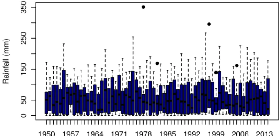
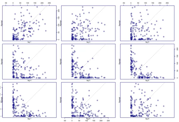
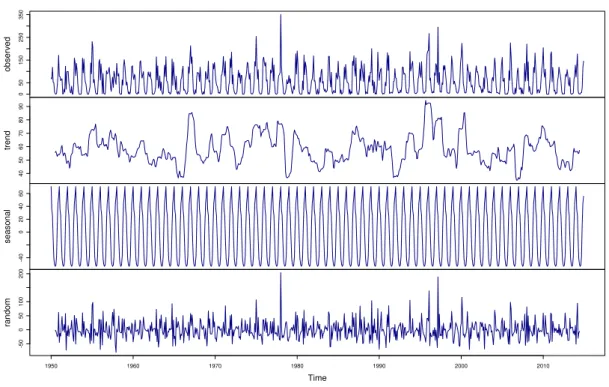
5.2.1 Data Exploration . . . 52
5.2.2 Model Identification and Fitting . . . 56
5.2.3 Model Accuracy . . . 59
5.3 Application to Temperature Data . . . 61
5.3.1 Data Exploration . . . 61
5.3.2 Model Identification and Fitting . . . 65
5.3.3 Model Accuracy . . . 67
6 Discussion and Conclusion 70 6.1 Introduction . . . 70 6.2 Summary of Findings . . . 70 6.3 Future Research . . . 71 References 73 A Additional Results 76 B R Code 81
List of Figures
2.1 Example of a time series . . . 15
2.2 Purely random process . . . 22
2.3 Random walk process . . . 23
4.1 Datasets Plots . . . 48
5.1 Rainfall Box-and-whisker plot . . . 54
5.2 Rainfall Lag Plot . . . 55
5.3 Rainfall Autocorrelation Plot . . . 56
5.4 Rainfall Classical Decomposition . . . 57
5.5 Temperature Box-and-whisker plot . . . 62
5.6 Temperature Lag Plot . . . 63
5.7 Temperature Autocorrelation Plot . . . 64
5.8 Temperature Classical Decomposition . . . 65
A.1 Rainfall time series plot in multiple panels . . . 76
A.2 Temperature time series plot in multiple panels . . . 77
A.3 Box-and-whisker plot for Temperature, 2014 . . . 77
A.4 Average Daily Temperature: 2000-2014 . . . 78
A.5 Average Monthly Rainfall: 2000-2014 . . . 78
A.6 Residual Plots: Rainfall . . . 79
A.7 Residual Plots: Temperature . . . 79
A.8 Actual versus in-sample fit: Rainfall . . . 80
List of Tables
3.1 Taxonomy of exponential smoothing methods . . . 42
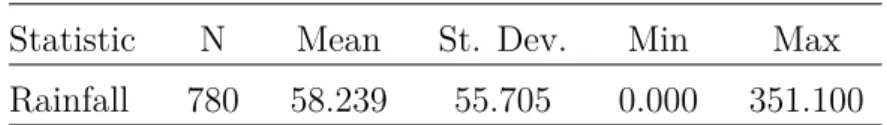
5.1 Descriptive Statistics: Rainfall . . . 53
5.2 Estimated Model Parameters: Rainfall . . . 58
5.3 In-Sample Accuracy Measures: Rainfall . . . 60
5.4 Out-of-Sample Accuracy Measures: Rainfall . . . 61
5.5 Descriptive Statistics: Temperature . . . 62
5.6 Estimated Model Parameters: Temperature . . . 66
5.7 In-Sample Accuracy Measures: Temperature . . . 68
Chapter 1
Introduction
1.1
Historical Overview
Exponential smoothing methods (ETS) have been used for time series forecasting and prediction since the 1950s. The methods are well known for their simple for-mulation and relative ease of use. In previous time series forecasting competitions [30, 29], exponential smoothing methods performed better than well developed and complex statistical methods like the autoregressive integrated moving aver-ages (ARIMA).
Exponential smoothing methods can be grouped into three basic classes: simple or single exponential smoothing, double exponential smoothing and triple expo-nential smoothing. A common characteristic of the methods is that the stochastic process that generated the observed data is a function of unobserved but deter-ministic components (e.g. local level, trend and season). The components need to be adjusted over time as the structure of the time series change.
The simple exponential smoothing method was developed independently by Brown [8] and Holt [21]. Winters [44] then extended the Holt exponential methods to
allow for forecasting complex time series including seasonality. Hence, the name Holt-Winters exponential smoothing methods to acknowledge their contribution. The original formulation of exponential smoothing methods was underpinned by
heuristics. Thus, they did not have a statistical basis for model selection as well as for modelling the distribution of the errors. However, their ease of use meant that businesses quickly adopted them, particularly those in inventory modelling. While the popularity of exponential smoothing methods increased from 1960 to 1970, the statisticians interest in the methods also grew. This was particularly motivated by the need to establish a statistical foundation for the methods. Two significant works laid the foundation for statistical investigations into exponen-tial smoothing methods. First, Muth [33] investigated the statistical properties of the simple exponential methods and found that the simple exponential smoothing method is the same as a model comprising of random walk and noise (i.e. random walk plus noise model [7]). Therefore, the simple exponential smoothing model could be modelled using a stochastic model. Second, Pegels [35] developed a clas-sification scheme of the exponential smoothing methods by considering variations in their trend and seasonal components. The classification later proved to be im-portant as a guide to research into statistical models underlying all the exponential smoothing methods.
However, Box and Pierce [5] developed a modelling strategy for autoregressive and moving average models (ARIMA [6]). The Box-Jenkins approach quickly emerged as a powerful statistical modelling framework. Most of the research in the 1970s
period was focused on the ARIMA. Research on exponential smoothing meth-ods carried out in this era was biased towards showing that some of exponential smoothing methods were special cases of the ARIMA models. Thus, ARIMA mod-els may have benefited from this research rather than the exponential smoothing methods.
Several papers in the 1980s were vital for the future of exponential smoothing methods. Gardner [16] provided a comprehensive review of exponential smooth-ing methods since they were formulated in the 1950s. In fact, Gardner [16] in-troduced new variations of exponential smoothing methods called damped expo-nential methods. The damped expoexpo-nential smoothing methods were developed to adjust the exponential forecasts downwards in long term forecasting. Snyder [41] demonstrated that the simple exponential smoothing method could be refor-mulated into a model that has one source of error. This type of reformulation is termed an innovation state space model. His work went largely unnoticed at the time [14].
Ord, Koehler, and Snyder [34] extended the innovations state space models to double and triple exponential smoothing methods building on the earlier work of Snyder [41]. Finally, Hyndman, Koehler, Snyder, and Grose [25] provided a comprehensive innovations state space framework for the exponential models. They were able to show that exponential smoothing methods belong to a class that is larger than that of the ARIMA methods. Gardner [17] reviewed the new developments in the exponential smoothing methods as a way of updating their previous work. The innovations state space framework is a major breakthrough for exponential smoothing methods. They can now be considered on equal footing with the ARIMA methods.
1.2
Motivation
Historically, exponential smoothing forecasting methods were viewed as heuristic
methods. They lacked a coherent statistical framework for modelling error dis-tribution. Thus, they received little attention from among statisticians. Some even considered them to be special cases within the ARIMA models [33,31]. This
situation is now different.
The development of an innovations1state space framework for exponential
smooth-ing methods is a major reason for this. The significance of innovations state space models is that statistical modelling using exponential smoothing methods can be done on an objective basis. Thus, the methods that were largely ignored by the statistical community can now be tested in various application areas. Weather forecasting is one potential application area of exponential smoothing methods. It is important to assess whether or not exponential smoothing methods can be used to forecast weather related data.
A rather indirect justification for undertaking this research is that of in-filing miss-ing weather related time series. If weather measurements are faulty at particular time points, then imputation methods can be used to fill in the missing obser-vations. A possible imputation approach is back forecasting with an exponential forecasting method. This is, however, not the main interest in this research but is something that could be explored further.
1.3
Aims and Objectives
This research report is primarily concerned with exploring the performance of different methods for smoothing time series. More specifically, the focus is on comparing the performance of the exponential smoothing techniques on historical temperature and rainfall data. Formally, the aim and objectives are as below.
1.3.1
Aim
The aim of the project is to compare the performance of exponential smoothing methods on two weather related data sets that exhibits trend and seasonality.
1.3.2
Objectives
• To present a review of exponential smoothing methods with specific emphasis
on the Holt-Winters methods,
• To perform forecasts using the exponential smoothing methods and assess
their performance through out-of-sample forecasting validation,
• To compare the performance of exponential methods against naive
smooth-ing methods on the two data sets, and
• To comment on the performance of exponential smoothing methods on the
two data sets.
1.4
Organization of the Report
The research report is structured as follows. Chapter 2 can be divided into two parts. The first part gives a theoretical background of stochastic processes as the umbrella statistical processes under which the research falls. The second part introduces general time series concepts which are the basic building blocks of the research project. Chapter3narrows down time series to focus solely on exponential smoothing forecasting methods. Chapter4deals with the data and actual methods used in the analysis. Chapter 5 presents the results of exponential smoothing forecasts. Chapter 6 concludes with a summary and discussion of possible areas for future research.
Chapter 2
Theoretical Background
2.1
Introduction
This chapter discusses the basic theory of stochastic processes and foundational aspects of time series. Section 2.2 introduces the basics of stochastic processes. We present the general case for stochastic processes, of which stochastic processes
in discrete time are a special case. In Section 2.5, we consider some important
concepts in time series. Section 2.6 describes discrete stochastic models for uni-variate time series. Section 2.7 deals with evaluating the accuracy of time series forecasts.
2.2
Stochastic Processes
Stochastic processes theory is very well developed in literature. In this section we give an overview of stochastic processes highlighting the aspects that are important in time series analysis. The material presented here is based largely on Beichelt [2], Grimmett and Stirzaker [20] and Ross [39]. These three monographs offer a non-measure theoretical approach to stochastic processes. The section begins with
the definition of a random variable and extends it to the notion of the stochastic process. Further, the characteristics of stochastic processes are introduced. The section ends with a discussion on classification of stochastic processes.
2.2.1
Random Variable
A random variableX refers to the possible values of a statistical experiment when the conditions are fixed [2]. As conditions are fixed, any deviation to the value of the random variable is attributable to chance alone. A change in the experimental conditions will affect its outcome. A random variable can be redefined to take into account the case when experimental conditions vary. A random function X(t) is a random variable depending on a parameter t where t is deterministic. This results in a generalization of random functions. The study of random functions is formalized next.
Let {X(t), t ∈T}denote a random variable X depending on a time parameter t
whose values are elements of a setT. The setTrepresents the sample space of the time parameter t. The set T can be either one-dimensional or multidimensional. In addition, assume Z to be the sample space for X(t) underT.
2.2.2
Stochastic Process
A collection of random variables{X(t), t∈T}with parameter space Tand state space Z is known as a stochastic process [2]. {X(t), t ∈T} is called a stochastic process in discrete-time if the parameter spaceT is countable. If parameter space
T is continuous, then {X(t), t ∈ T} refers to a stochastic process in
continuous-time. Depending on the state spaceZ, a stochastic process can also be discrete or continuous. Thus, if the state space Z is countable, then {X(t), t ∈T} refers to a stochastic process indiscrete-space. Similarly, if the state space Zis continuous,
then the stochastic process is called a stochastic process in continuous-space. By and large, the set Tand the state spaceZ result in four distinct types of stochas-tic processes. Time series are an example of a continuous-space stochasstochas-tic process in discrete-time or continuous-space stochastic process in continuous-time. Other examples include Poisson processes which are discrete-space stochastic processes in continuous-time, diffusion processes which is a continuous-space stochastic pro-cesses in continuous-time and discrete-time Markov chains which are discrete-space stochastic processes in discrete-time.
2.3
Characteristics of Stochastic Processes
A stochastic process {X(t), t∈T}is fully characterized by its finite-dimensional distribution. The finite-dimensional distribution of a stochastic process{X(t), t∈
T} is the family of all joint probability distributions of (X(t1), X(t2), . . . , X(tn))
and is given by the n-dimensional distribution functions
Ft1,t2,...,tn(x1, x2, . . . , xn) = P(Xt1 < x1, Xt2 < x2, . . . , Xtn < xn) (2.1)
where n = 1,2,3, . . . and t1, . . . , tn ∈ T. Modelling the dependence between any
sequence of random variables X(tn) in a generalized random experiment depends
on this complete statistical or probability characterization. The study of the nature of time dependence between random variables is a subject of research in time series.
2.3.1
Sample Path
A sample path of a stochastic process{X(t), t∈T}is any realization{x(t), t∈T}
sample path describes one instance of a dynamic stochastic system. Thus, sample paths model the possible developments of the stochastic system.
2.3.2
Trend Function
The trend function m(t) of a stochastic process {X(t), t ∈ T} refers to the ex-pected value of X(t). It depends on the time parameter, t. In mathematical notation, it is represented as
m(t) = E(X(t)), t∈T. (2.2)
There are two possible interpretations of m(t). Using theory of probability, the Law of Large Numbers [15] states that the arithmetic mean of many independent observations x(t) at the same time point twould be approximately equal to m(t). The trend function m(t) can also be interpreted as the average of the realization
x(t) over time. If the probability density function ft(x) exist, then it is given by
m(t) =
Z +∞
−∞ xft(x)dx, t ∈T. (2.3)
2.3.3
Covariance Function
The (auto)covariance function C(s, t) of a stochastic process{X(t), t∈T}refers to the covariance between two random variablesX(s) andX(t) expressed in terms of s and t. Hence, the covariance function measures the degree of statistical dependence between X(s) and X(t). The covariance function C(s, t) is given by
Further simplification yields
C(s, t) = E(X(s)X(t))−m(s)m(t); s, t∈T. (2.5)
In the case of t =s, we have the formula for thevariance of a stochastic process
{X(t), t∈T} as given by
C(t, t) =V ar(X(t)) =E[X(t)−m(t)]2; s, t ∈T. (2.6)
2.3.4
Correlation Function
The (auto)correlation function ρ(s, t) of a stochastic process {X(t), t∈T}refers to the correlation between two random variablesX(s) andX(t) expressed in terms of s and t. It is important in modelling the development of a stochastic process through time. The covariance function ρ(s, t) is given by
ρ(s, t) = q Cov(X(s)X(t))
V ar(X(s))qV ar(X(t))
(2.7)
The terms autocovariance and autocorrelation refer to the fact that we are deal-ing with the same stochastic process at different time points. If, however, we are interested in the covariance and correlation between two different stochastic pro-cesses, say {X(t), t ∈ T} and {Y(t), t ∈ T}, then such functions will be better defined ascross covariance function and cross correlation function. The formulae remain the same as the above. Autocorrelation and autocovariance functions are very useful in time series model identification.
2.4
Classification of Stochastic Processes
Stochastic processes can be classified by making use of theirn-dimensional distri-butions. However, this requires a simplified probability structure since it is im-possible to observe all im-possible sample paths of the stochastic processes. Beichelt [2] argues that stochastic processes are classified according to their steady-state properties. That is, a stochastic process is characterized when its statistical prop-erties are invariant with time. This is called a stochastic process in stationary or steady-state. Not all stochastic processes have the stationarity property. Thus, stationary stochastic processes can be viewed as a subset of the set of all stochas-tic processes. In a way, stationarity reduces the class of stochasstochas-tic processes and allows for inference of the entire stochastic process. Stationarity is formalized next.
2.4.1
Stationary Processes
Strict Stationarity
A stochastic process {X(t), t ∈ T} is defined as strictly or strongly stationary if joint distribution functions of random vectors
(Xt1, Xt2, . . . , Xtn) and (Xt1+u, Xt2+u, . . . , Xtn+u) (2.8)
are identical for all t, possible integer n, and t1, t1, . . . , tn ∈T satisfying the
con-ditions tj +u∈T, j = 1, . . . , n. That is,
This means that a stochastic process is strongly stationary if joint distribution functions of a set of random vectors is not changed with a displacement in the time origin,u. A strongly stationary process is not very useful for practical applications since it is very difficult to verify that a process is strongly stationary. This gives rise to the concept of weakly stationary processes.
Weak Stationarity
A stochastic process {X(t), t∈T} is referred to as weakly or wide-sense stationary if it satisfies the following conditions:
• E|X(t)|2 <∞for all t∈
T
• m(t) = E(X(t)) =µ for all t∈T where µis a constant, and
• C(s, t) = C(0, t−s) for all s, t ∈Twhere C(s, t) = Cov(X(s)X(t)).
In other words, a stochastic process is weakly stationary if it has finite first and second moments and a covariance function that depends only on the interval length (i.e. covariance stationary). The (auto)covariance function for a stationary stochastic process {X(t), t ∈ T} can be written as C(s, t) = C(0, t−s) for all
s, t∈T. Therefore, the (auto)covariance function of the process can be expressed in terms of just one variable τ as
C(τ)≡C(0, τ) = Cov(X(t+τ)X(t)) for all t, τ ∈T. (2.10)
2.4.2
Homogeneity and Independent Increments
Homogeneous Increments
A stochastic process {X(t), t∈T} is said to have homogeneous increments if, for arbitrary but fixed t1, t2 ∈T, the increment X(t2 +τ)−X(t1 +τ) has the same
probability distribution for all τ with property t1+τ ∈T, t2 +τ ∈T.
Independent Increments
A stochastic process {X(t), t∈ T} is said to have independent increments if for alln= 2,3, . . . and for all n−tuples (t1, t2, . . . , tn)∈Tand t1 < t2 <· · ·< tn, the
increments
X(t2)−X(t1), X(t3)−X(t2), . . . , X(tn)−X(tn−1) (2.11)
are independent random variables.
2.4.3
Gaussian Processes
A stochastic process {X(t), t∈ T} is said to be Gaussian if the random vectors (X(t1), X(t2), . . . , X(tn)) have multivariate normal distributions for all n−tuples
(t1, t2, . . . , tn) ∈ T and t1 < t2 < · · · < tn; n = 1,2, . . .. That is, all
finite-dimensional distributions of the process are joint Gaussian distributions. If µ= (µt1, µt2, . . . , µtn)
0 be the mean vector andΣ denotes then×n covariance matrix
of the process, then the probability density function of the multivariate normal distribution is given by:
f(x) = (2π)−n2|Σ|− 1 2 exp{−1 2(x−µ) 0 Σ−1(x−µ)} (2.12)
where |A| is the determinant of a quadratic matrix A. The covariance matrix
must also be positive definite. An important characteristic of a Gaussian process is that its finite-dimensional distribution is fully characterized by its first and second moments. This means that it is characterized by its mean and covariance functions. In this special case, weak stationarity implies strong stationarity. The
reverse is always true if the underlying stochastic process is a second order process.
2.4.4
Markov Processes
A stochastic process {X(t), t ∈ T} in discrete state space is said to have the Markov(ian) property if for all (n+ 1)−tuples (t1, t2, . . . , tn+ 1) ∈ T, t1 < t2 <
· · ·< tn+1 and j,
P{X(tn+1) =j|X(t0) =i0, X(t1) = i1, . . . , X(tn) =i}=P{X(tn+1) = j|X(tn) =i}.
(2.13) In non-technical terms, the Markov property states that the probability of any future behaviour of a stochastic process, if the current state is exactly known, will not be changed by information concerning the process’ past behaviour.
2.5
Univariate Time Series
This section outlines the general context in which our study of time series analysis takes place. We restrict our context to time series in time domain only. We begin by defining the elementary concepts associated with time series. Then Section
2.5.3 introduces the notion of classical decomposition, setting the scene for the rest of the report. The section ends by introducing the concept of smoothing in time series. All the concepts introduced in this section can be considered to be primary tools for time series modelling.
2.5.1
Time Series as a Stochastic Process
A time series is a set of realized values of a stochastic process {X(t), t ∈ T}
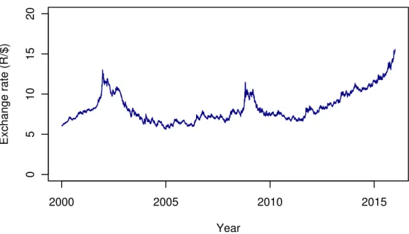
sample path of a stochastic process if you stick to the strict definition above. Dagum [13] notes that, unlike in cross sectional studies, in time series analysis ordered observations are dependent through time. That is, observations are related through their index in time. Dagum [13] also states that the time dependence of observations is of importance in time series. A question that often arises in time series is what constitute a time series: the data or the data generating process? Brockwell and Davis [7] suggest that both the data and data generating process of which the time series is a sample path can be referred to as a time series. Figure
2.1 shows a time series plot of the Rand/Dollar exchange rates over the period 2000 and 2015. The exchange rates fluctuates between R5 and R15 per $1. A
2000 2005 2010 2015 0 5 10 15 20 Year Exchange rate (R/$)
Figure 2.1: Example of a time series
stochastic process approach to time series modelling requires that observed time series data be treated as a finite component of a sample path. Then, the stochastic model serves as the theoretical model that generated the data series. This view of time series allows the use of the theoretical models developed for probability
and stochastic processes. In essence, all the properties of stochastic processes mentioned in Sections2.2,2.3 and 2.4 are applicable to time series. In particular, the concept of stationarity is very much central to time series modelling.
2.5.2
Wold Decomposition Theorem
The Wold Decomposition Theorem is an important theorem in time series. Put simply, the theorem states that any discrete stationary stochastic process can be expressed as a superposition of a purely deterministic process and a purely non-deterministic process [7]. A purely deterministic process, such as a function of time, is always uncorrelated to any other genuine stochastic processes. Also, a deterministic process is a general stochastic process. Any stationary process {X(t), t ∈ T} of which µ is the expected value can be decomposed into two uncorrelated components: X(t) = Z(t) +V(t), cov(Z(t), V(t))≡0, ∀t∈T (2.14) where V(t) =µ+ ∞ X j=1 [αjsin(λjt) +βjcos(λjt)], 0< λj ≤π (2.15) Z(t) = ∞ X j=0 Ψjat−j, Ψ0 = 1, ∞ X j=1 Ψ2 ≤ ∞ (2.16)
where at is a white noise process and αj and βj are sequences of uncorrelated
random variables with mean zero ∀j. An application of the Wold Decomposition Theorem is found in the classical decomposition of time series.
2.5.3
Classical Decomposition
Classical decomposition of a time series has its origins in the work of Persons [36] and Persons [37]. His work on developing business indices was among the first to explicitly define the generating processes of a time series. While there has been lots of developments in time series analysis ever since, the classical decomposition method has remained largely unchanged. The method proposes the components of the stochastic process underlying a general time series. It states that any time series {X(t), t ∈ T} can be expressed as a function of its major components. Chatfield [12] lists the components as:
• Trend Component (T(t)) which accounts for the long term increase or
de-crease in the mean of the series,
• Seasonal Component (S(t)) which accounts for cyclical fluctuations related to calendar time (e.g. hour, day, month or quarter),
• Cycle Component (C(t)) which accounts for other cyclical fluctuations (e.g. business cycles) which may or may not be permanent, and
• Random Noise Component (R(t)) which measures other random fluctuations
and is assumed to be stationary.
In practice, trend and cycle components of a time series can be combined into trend-cycle. ComponentsT(t), S(t) andC(t) are deterministic whileR(t) is non-deterministic thereby satisfying the Wold Decomposition Theorem. Brockwell and Davis [7] argue that the aim of classical decomposition is to estimate the deterministic components and if the model is correct the random noise component would be a stationary random process. In mathematical notation, the stochastic process underlying a time series is given by:
Traditionally, the sources of variations in a time series have been assumed to be deterministic and therefore independent of each other. Hence, the time series can be specified by means of an additive superposition model as:
X(t) = T(t) +S(t) +C(t) +R(t) (2.18)
where X(t) denotes the observed series at time t, T(t) the trend component at time t, S(t) seasonal component at time t, C(t) is the cycle component at time
t and R(t) the random noise or irregular component at time t. The additive decomposition model is appropriate in situations where the amplitude of seasonal component S(t) does not change with changes in time series level.
There are cases when the additive model is not suitable. For example, when there is dependence among the underlying components of the stochastic process. That is, the amplitude of the seasonal component S(t) varies with the level of the time series. In such cases, decomposition is specified through a multiplicative model as follows
X(t) =T(t)S(t)C(t)R(t) (2.19) where nowS(t) andR(t) are expressed in proportion to the trendT(t) andC(t). A logarithmic transformation makes this model an additive model (i.e. log(X(t)) = log(T(t)) + log(S(t)) + log(C(t)) + log(R(t))). A third group of decomposition models makes use of a combination of the additive and multiplicative models. An example of such models is the pseudo-additive model given below
Y(t) = [T(t) +S(t) +C(t)]R(t) (2.20)
where the variables are as mentioned above. Seasonally adjusted time series can be formed by removing the seasonal componentS(t) from observed data. This results in a time series Y∗(t) which is a function of trend and random error components
only. The seasonal adjusted time series are Y∗(t) = Y(t) −S(t) and Y∗(t) =
Y(t)/S(t) for the additive and multiplicative models respectively.
2.5.4
Types of Smoothing
Smoothing techniques are efficient methods to identify important and non-important fluctuations within an observed time series. The techniques allow for easy iden-tification of the trend component T(t) of the series. Smoothing is an important element of time series forecasting. Smoothing theory presented here is based on Chatfield [12] and Shumway and Stoffer [40]. Smoothing has its origins in the theory of linear systems. A linear filter maps a given time series {xt, t∈T} into
a new time series {yt, t∈T}as follows:
yt= ∞
X
j=−∞
wjxt−j, t∈T. (2.21)
where wj are the filter weights assigned to the values xj of a time series. For a
given interval, say [−a, b], the weights satisfy the following normalizing condition:
b
X
j=−a
wj = 1 (2.22)
The interval [−a, b] determines the bandwidth of the filter.
Moving Average Smoothing
The moving average is a type of a linear filter with the interval [−a, a] with 2a+ 1 time points. The weights assigned by a moving average smoother are all the same and equal to wj = 1 2a+1 for j =−a,−a+ 1, . . . , a−1, a 0 Otherwise. (2.23)
Kernel Smoothing
Kernel smoothers are sometimes referred to as density estimators. Examples in-clude the Gaussian and Epanechnikov kernels. The Gaussian kernel uses the Gaus-sian (normal) distribution function as the weights. The weights for the Epanech-nikov kernel using the bandwidth [−a, a] are given by
wj =c " 1− j 2 (a+ 1)2 # for j = 0,±1, . . . ,±a. (2.24)
Ideally, the wider the bandwidth the smoother the kernel. In order forPa
j=−awj =
1 to be satisfied, it follows that the factor c is given by
c= " a(4a+ 5) 3(a+ 1) #−1 (2.25) Exponential Smoothing
In exponential smoothing, the past and present values of a time series {xt, t ∈
1. . . n} are used to calculate yk from the observations xk, xk−1, . . . , x0 according to the following rule
yk=λl(k)xk+λ(1−λ)l(k)xk−1+· · ·+λ(1−λ)kl(k)x0, k= 0,1, . . . , n. (2.26)
where the parameterλsatisfies 0< λ <1. The weights under exponential smooth-ing are given by
The bandwidth is such thata=a(k) = k+ 1 andb = 0. In order forPb
j=−awj = 1
to be satisfied, it follows that the multiplier c(k) is given by
c(k) = 1
1−(1−λ)k+1 (2.28)
If the parameterλis small, this implies a strong smoothing onxjsince observations
that are far in time will have a non-negligible effect on smoothing. Exponential smoothing methods for forecasting are dealt with in depth in Chapter 3.
2.6
Models for Discrete Time Series
This section describes stochastic processesin discrete timethat are useful for time series modelling. A more detailed discussion of the probability models described here can be found in Beichelt and Fatti [3] and Chatfield [12]. Unless stated otherwise, the information presented in this section comes from these two books.
2.6.1
Purely Random Process
A stochastic process indiscrete time is defined as a purely random or white noise
process if it is made up of a sequence of independent and identically distributed random variables{t}. The random variables{t}are assumed to be from a normal
distribution with mean zero and variance σ2. Thus, a purely random process has constant mean and variance. The covariance function of a purely random process is given by γ(k) =Cov(t, t+k) = σ2 k= 0 0 k=±1,±2, . . . (2.29)
The mean and autocovariance function of a purely random process are independent of time. This means that a purely random process is covariance stationary. The
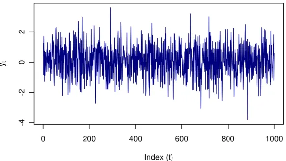
assumption of independence guarantees that the process is also strictly stationary. The purely random process is not particularly interesting in itself but can be used to build more complex time series (e.g. autoregressive moving averages). Figure
2.2below shows an example of a purely random process simulated from a standard normal distribution. 0 200 400 600 800 1000 -4 -2 0 2 Index (t) yt
Figure 2.2: Purely random process
2.6.2
Random Walk
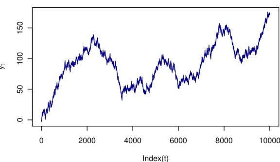
Lett denote a discrete-time, purely random process having mean µand variance
σ2. The process {Yt} is called a random walk if
Yt=Yt−1+t. (2.30)
By convention, the process starts at zero when t = 0 so that Y1 = 1 and Yt =
Pt
thus the process is not stationary. A first difference of the random walk process,
5Yt = t, results in a purely random process and therefore the first difference of
a random walk is stationary. This insight is important in modelling time series
whose behaviour is a random walk such as is the movement in share prices in successive time periods. An example of random walk process is shown in Figure
2.3 below. 0 2000 4000 6000 8000 10000 0 50 100 150 Index(t) yt
Figure 2.3: Random walk process
2.6.3
Autoregressive Process (AR)
A stochastic process {Yt} is called an autoregressive process of order p, denoted
by AR(p), if it is defined by Yt= p X i=1 φiYt−i+t (2.31)
where p is an integer, φ1, . . . , φi are fixed constants of the autoregressive terms
and {t} denotes a sequence of independent random variables with mean 0 and
variance σ2. The model is similar to multiple linear regression with the exception that Yt is regressed on historical values of Yt rather than on separate predictors.
If p = 1, the AR(1) process is called a first-order AR process and is defined by
Yt = φ1Yt−1+. When p > 1, the process is a general order AR process. Upon applying the backward shift operator BYt =Yt−1, AR(p) becomes
(1−φ1B −φ2B2− · · · −φpBp)Yt=t (2.32)
which can be written compactly as φ(B)Yt =t where
φ(B) = 1−φ1B−φ2B2− · · · −φpBp (2.33)
is called the autoregressive operator andYt=φ(B)−1tis an infinite series. {Yt} is
covariance stationary if all the roots of the equationφ(B) = 0 lie outside the unit circle. A necessary condition for stationarity is that Pp
i=1φ < 1. Autoregressive processes are useful for modelling time series whereby the current value is linearly related to its preceding value plus some random noise.
2.6.4
Moving Average Process (MA)
A stochastic process {Yt} is called a moving average process of order q, denoted
by MA(q), if it satisfies Yt= q X j=0 θjt−j (2.34)
where q is an integer, θ1, . . . , θq are fixed constants of moving average process,
θ0 = 1 and{t}is a sequence of independent random variables such that mean is 0
by Yt=θ0t+θ1t−1. When q >1, the process is a general order MAprocess. It is clear that E(Yt) = 0 and V ar(Yt) = σ2
Pq
i=0βi2, because 0
js are independent.
The covariance function of the MA(q) is given by
γ(k) = Cov(Yt, Yt+k) = 0 k > q σ2 Pq−k i=0 θiθi+k k = 0,1, . . . , q γ(−k) k < 0. (2.35)
The mean and covariance of MA(q) are independent oftso the process is covariance stationary for all values of θ. If the t are normally distributed then the MA(q)
will be strictly stationary. Using the backward shift operator,B, the MA equation can be expressed in the form
Yt=θ(B)t (2.36)
where θ(B) = 1−θ1B−θ2B2 − · · · −θpBq. Unlike the autoregressive processes,
there is no restriction on the θi for stationarity. However, for the process to be
invertible, the roots of the polynomial θ(B) = 0 must lie outside of the unit circle. This means that a moving average process can be expressed in terms of an autoregressive process whose coefficients satisfy θ(B) = 0.
The moving average process MA(q) is a finite stochastic process because the order
q is an integer. When the order is unbounded, we have a moving average process of unbounded denoted by MA(∞). A stochastic process is an MA(∞) if it can
be expressed as Yt = P∞j=0θjt−j and provided that P∞j=0θ2j converges. The
im-portance of an MA(∞) is that any AR(p) can be expressed as MA(∞). Similarly, subject to being an invertible process, an MA(q) can be expressed as AR(∞).
2.6.5
Autoregressive Moving Average Process (ARMA)
A new class of time series models is formed by combining AR and MA processes.
An autoregressive moving average process, ARMA(p, q) of a time series Yt is
de-fined by Yt = p X i=1 φiYt−i+ q X j=0 θjt−j (2.37)
where p is the number of AR terms, q is the number of MA terms, φ refers to the coefficients of the AR terms, θ refers to the coefficients of the MA terms and constant and {t} is a purely random process. Using the backward shift
operator,B, the equation above can be expressed in the form
φ(B)Yt=θ(B)t (2.38)
whereφ(B) = 1−φ1B−φ2B2−· · ·−φpBp andθ(B) = 1−θ1B−θ2B2−· · ·−θpBq.
The values of {φi} and {θi} which make the process stationary are the roots of
φ(B) = 0 and θ(B) = 0 respectively. All the roots must lie outside of the unit circle. The ARMA(p, q) is very flexible in that stationary time series can be modelled using an ARMA with fewer parameters than a pure AR or MA on its own.
2.6.6
Integrated ARMA Process (ARIMA)
An autoregressive integrated moving average process, ARIMA(p, d, q), is an
ex-tension of the ARMA process to data that are not stationary. If data are non-stationary, then it is necessary to make it stationary before an ARMA can be applied to the data. One common method of making a time series stationary is by differencing the series, expressed as 5dY
t. d denotes the number of differences to
5dY
t in the ARMA model then the model is referred to as an integrated model.
The term integrated is due to the fact that a stationary model has been fit to differenced data have to be summed to provide a model for the original data (i.e. non-stationary). Integration is a form of summing, hence the term. A time series
Yt is said to be of the ARIMA(p, d, q) if 5dYt is a stationary ARMA process and
the parameters as stated previously. The general ARIMA model is of the form
φ(B)(1−B)dYt=θ(B)t (2.39)
whereB, φ(B) and θ(B) are as in ARMA. A generalization of the ARIMA model to deal with non-seasonal data is found in Box and Pierce [5]. Such a model is referred to as a SARIMA.
2.6.7
General Linear Process
A general class of linear processes may be written as a moving average process, of possibly infinite order, in the form
Yt= ∞
X
i=0
φXt−i. (2.40)
A sufficient condition for the sum to converge and hence the process to be sta-tionary is that P∞
i=0|φ| < ∞. Stationary AR and ARMA processes can also be expressed in terms of the general linear process.
2.6.8
Box-Jenkins Forecasting with ARIMA
The Box-Jenkins procedure [6] is a forecasting strategy based on the autoregressive integrated moving average (ARIMA) models. It emphasizes an iterative process to forecasting model building as follows:
1. Model identification Explore the data to select a suitable model from the ARIMA family,
2. Estimation Estimate model parameters for the selected model,
3. Diagnostic checking Assess residuals from the fitted model to see if it does
not violate model assumptions, and
4. Consideration for alternative models If the chosen model is not adequate,
repeat the above process until a suitable model can be found.
2.7
Forecasting in Time Series
Forecasting refers to the process of estimating the future trajectory of a sequence of observations (i.e. how the time series will continue into the future).
2.7.1
Portmanteau Tests
When fitting a time series model the distribution of residuals is of importance to the modeller. We are interested in finding whether or not the residuals of the estimated model are white noise. A plot of the autocorrelation function (ACF) can show if the residuals are uncorrelated, have mean zero and constant variance. However, it is often not sufficient. A portmanteau test is a formal test for the independence of residuals up to a lag m. The most commonly used portmanteau tests are described below.
Box-Pierce Test
This classical test was proposed by Box and Pierce [5]. The test statistic for Box-Pierce test is given by
Q=n
m
X
k=1
rk2 (2.41)
where rk is sample autocorrelation of order k, m is the maximum lag considered
and n is the number of observations. Under the null hypothesis that the model is adequate (i.e. residuals are white noise), Q follows the χ2 distribution with (m−P) degrees of freedom. The constant P is a count of model parameters. If the rk0s are very small (i.e. close to zero), then the value of Q will be small. If some rk0s are large, then Q will be large. The Box-Pierce test performs poorly in small samples.
Ljung-Box Test
Ljung and Box [27] developed an alternative test to deal with the perceived short-comings of the Box-Pierce test. Their test is designed to work well with small samples. The test statistic for the Ljung-Box test is given by
Q∗ =n(n+ 2) m X k=1 r2k n−k (2.42)
whererk is sample autocorrelation of orderk, m denotes the maximum lag andn
is the total observations. Under the null hypothesis that the residuals are white noise,Q∗ follows theχ2 distribution with (m−P) degrees of freedom whereP is a count of parameters in the model. If therk0s are small (i.e. in the neighbourhood of zero), then Q∗ will be small. Conversely, if some r0ks are large, then Q∗ will be large.
2.7.2
Cross Validation
Measuring how well a statistical algorithm (method) performs on a given dataset is an integral part of statistical modelling. A common approach is to train (fit) an algorithm to a dataset and then use the fitted model to predict the observed values. The extent to which the predicted values deviates from the observed values gives a measure of performance of the method. This kind of approach evaluates the method on the full dataset and may yield downward biased estimates. The cross
validationapproach was developed to deal with perceived weaknesses of evaluating
an algorithm on same data it was trained on [26,32,42, 18]. In its simplest form,
cross validation involves splitting a dataset into two sub-datasets. The split ratio depends on the features and size of the dataset, though a ratio of 70 : 30 is usually recommended. One of the datasets is used to train the algorithm and the other is used to evaluate its statistical performance. If a split is performed only once, it gives a validation estimate while averaging over multiple splits it is known as a
cross validation estimate. Often an assumption is made that the sub-datasets are
independent and identically distributed.
The approach to cross validation described above fails when data are dependent, such as is time series data. This is because observations left out during training of the algorithm are necessarily correlated with those used in the training of it. Asso-ciated information therefore remained in the evaluation data making it difficult to assess the performance of the algorithm (method). However, Burman, Chow, and Nolan [10] demonstrate that cross validation can be extended to the dependent data, where the data form a stationary sequence. They suggest an h−block cross
validation obtained by removing h observations in the neighbourhood of the test
observation. Arlot and Celisse [1] provide a comprehensive survey of research into
cross validation for both independent and dependent data.
fol-lowing method tocross validation:
• Fit a time series model to the dataY1, . . . , Yt,
• Let ˆYt+1 be the forecast value of the next time point,
• Calculate the forecast error (e∗t+1 =Yt+1−Yˆt+1) for the forecast value,
• Redo the process for t = m, . . . , n−1 where m is the smallest number of observations needed to fit the model and
• Calculate forecast accuracy measures (e.g. mean square error) frome∗m+1, . . . , e∗n.
2.7.3
Forecast Accuracy Measures
The performance of an exponential smoothing method is assessed by considering its forecasting accuracy. There are a number of evaluation criteria which are used to estimate forecast accuracy [24]. Hyndman and Athanasopoulos [22] provide a useful grouping for forecasting accuracy measures. They classify forecasting accuracy measures as scale-dependent, percentage and scaled. We present six accuracy measures used in this report, according to the grouping.
Scale Dependent Measures
Scale dependent accuracy measures are measures which are based on the same scale as the data values. They are, therefore, sensitive to the data values. The forecast error itself is based on the data values and thus is scale dependent. Any accuracy measure that is a function of the forecast error only and not the data values is scale dependent. This means such accuracy measures can not be used for comparing time series measured on different scale. The most common scale dependent measures are defined below. Mean Error (ME) is calculated as the
average of the forecast errors over n observations. ME = 1 n n X t=1 et (2.43)
Mean Absolute Error (MAE) is calculated as the average of the absolute forecast
error values over n data points.
MAE = 1 n n X t=1 |et| (2.44)
Mean Square Error (MSE)is calculated as the average of the total squared forecast errors overn data points.
MSE = 1 n n X t=1 e2t (2.45)
Root Mean Square Error (RMSE)is calculated by taking the square root of MSE
(i.e. q(M SE)).
Percentage Measures
Percentage accuracy measures are independent of measurement scale. Thus, they are suitable for comparing the performance of time series that are measured on different scales. The common ones include the mean percentage error and mean absolute percentage error. They are undefined on time series with zero values and give extreme estimates with data values in the neighbourhood of zero. Mean Percentage Error (MPE)is the average of forecast errors with respect to the actual values over n data points.
MPE = 1 n n X t=1 et yt (2.46)
Mean Absolute Percentage Error (MAPE) is calculated by taking the average of forecast errors with respect to the true values over n data points.
MAPE = 1 n n X t=1 |et| yt (2.47) Scaled Measures
The scaled measures deal with the weaknesses of the percentage errors [24]. They do not become undefined or produce extreme values. A common scaled measure is the mean absolute scale error defined below. Mean Absolute Scaled Error (MASE)
is the average absolute error produced by the actual forecast over n data points.
MASE = 1 n n X t=1 |et| 1 n−1 Pn−1 i=2 |yi−yi−1| ! (2.48)
By and large, all the accuracy measures are based on how close the forecasts are to the eventual (or observed) outcomes. In practical applications, however, the measures are known to give completely different results. As such, evaluating the accuracy of a time series require that one use more than one accuracy measure.
2.7.4
Prediction Intervals
A prediction interval (PI) measures the extent of uncertainty around forecast
or predicted values. It consists of lower and upper bounds which a forecast or predicted value is expected to be bounded with a specified confidence level. The PI is dependent on the forecasting method used. The 100(1 −α)% prediction interval for yt+h is given by
ˆ
yt(h) ± zα/2
q
where t(h) = yt+h−yˆt(h) is the forecast error made at time t when forecasting
h steps ahead, zα/2 is a multiplier from the standard normal distribution at α/2 and V ar is the variance of the errors.
Chapter 3
Exponential Smoothing Methods
(ETS)
3.1
Introduction
The main idea behind the exponential smoothing method is to smooth a time se-ries by allocating more importance to recent observations and less importance to observations that are located far in time. It does so by allocating unequal weights to the observations. The largest weight is given to the current observation, less weight to the immediately preceding observation, even less weight to the obser-vation before that, and so on. The weights assigned to time series obserobser-vations older in time decrease exponentially. By and large, exponential smoothing de-pends more on recent observations than old observations to forecast. Exponential smoothing methods have three main forms: single exponential smoothing, double exponential smoothing and triple exponential smoothing methods. General expo-nential smoothing (GES) methods are less well known but are also discussed at the end. Differences between Holt-Winters and GES methods are highlighted.
3.2
Single Exponential Smoothing
This method is commonly known as simple exponential smoothing (SES). The terms are used interchangeably in this report. Simple exponential smoothing is mainly used for short-term forecasting, usually for periods not longer than one month [12]. The method assumes that the time series fluctuates around a stable mean (i.e. the time series is stationary). Thus, there is no trend or seasonality in the time series. The general formula for simple exponential smoothing is:
Yt=αXt+ (1−α)Yt−1 (3.1)
where Yt is the smoothed current smoothed value, Xt is the current observation
and α is a smoothing parameter such that 0< α < 1. In the SES, setting of the initial value ofYtis critical. A recursive application of the method shows that the
weights decay geometrically.
Yt=αXt+ (1−α)Yt−1 (3.2)
=αXt+ (1−α)[αXt−1+ (1−α)Yt−2] (3.3) =αXt+α(1−α)Xt−1+ (1−α)2Yt−2 (3.4) =αXt+α(1−α)Xt−1+α(1−α)2Xt−2+· · ·+α(1−α)t−1X1+ (1−α)tY0
(3.5)
The weights assigned to past observations are proportionate to terms in the ge-ometric series {1, (1−α), (1−α)2, (1−α)3, . . .}. The geometric series is the discrete case of the exponential function, hence the name exponential smoothing. The forecast equation for the SES is given by:
wherehis the number of forecast steps into future and its associated forecast error at timet is
et+h|t=Xt+h−Ft+h|t =Xt+h−Yt. (3.7)
Simple exponential smoothing smoothing can also be seen as updating the local mean level of a time series, Lt. This simply means replacingYtbyLtin the above
equations. This notation and interpretation is used in the next method.
3.3
Double Exponential Smoothing
Double exponential smoothing is a generalization of exponential smoothing to time series showing both changing local level and trend. The method is commonly known as Holt’s method. It involves exponentially updating (or adjusting) the level and trend of the series at the end of each period. The level (Lt) is estimated
by the smoothed data value at the end of each period. The trend (Tt) is estimated
by the smoothed average increase at the end of the period. The equations for updating the level and trend of the series are:
Lt=αXt+ (1−α)(Lt−1+Tt−1), 0< α <1 (3.8)
Tt =γ(Lt−Lt−1) + (1−γ)Tt−1, 0< γ < 1 (3.9)
where α and γ are smoothing parameters for level and trend respectively. The values of α and γ need not be the same. The forecast equation of the Holt’s method at timet is given by:
wherehis the number of forecast steps into future and its associated forecast error at timet is given by
et+h|t=Xt+h−Ft+h =Xt+h−Lt−hTt. (3.11)
3.4
Triple Exponential Smoothing
Triple exponential smoothing extends the double exponential smoothing to model time series with seasonality. The method is also known as the Holt-Winters in recognition of the name of the inventors. Winters improved the Holt’s method by adding a third parameter to deal with seasonality. Thus, the method allows for smoothing time series when the level, trend and seasonality can vary. There are two main variations of the triple exponential model and they depend on the type of seasonality. Section 2.5.3 has alluded to the seasonality models as additive or multiplicative model. If the seasonality is multiplicative (i.e. non-linear), then the three smoothing equations pertaining to level, trend and seasonality of p-period cycles are given by:
Lt=α(Xt/It−p) + (1−α)(Lt−1+Tt−1) (3.12)
Tt=γ(Lt−Lt−1) + (1−γ)Tt−1 (3.13)
It=δ(Xt/Lt) + (1−δ)It−p) (3.14)
where It is seasonality adjusting equation, p is the number of period in seasonal
cycle andδis its smoothing parameter such that 0< δ <1. The forecast equation
h-steps ahead at time t from the Holt-Winters with multiplicative seasonality is given by
and its associated forecast error at time t is
et+h =Xt+h−Ft+h =Xt+h−(Lt+hTt)It−p+h. (3.16)
If the seasonality is additive (i.e. linear), the smoothing equations are given by
Lt=α(Xt−It−12) + (1−α)(Lt−1+Tt−1) (3.17)
Tt=γ(Lt−Lt−1) + (1−γ)Tt−1 (3.18)
It=δ(Xt−Lt) + (1−δ)It−p (3.19)
where It is seasonality adjusting equation and δ is its smoothing parameter such
that 0< δ <1. Hyndman and Athanasopoulos [22] note that the additive model is seldom used in practice. The forecast equation at timet from the Holt-Winters method with additive seasonality is given by
Ft+h =Lt+hTt+It−p+h, h= 1,2,3, . . . (3.20)
and its associated forecast error at time t is
et+h =Xt+h−Fx+h =Xt+h−Lt−hTt−It−p+h. (3.21)
All the three main exponential methods are relatively simple to apply, with the SES being the simplest. However, it can be seen as the least realistic for application to real world time series. The exponential methods have been extended to include a “damping” factor which allows for a more conservative forecasting horizon [16,22]. The exponential smoothing methods are based on recurrence relations. They require initial values of the series of the recurrence equation to be set first. That is, the initial value of Yt in the SES, the initial values of Lt and Tt in Holt’s