and Interpretable Spatial Analysis
Jung Yeon Park1 Kenneth Theo Carr1 Stephan Zheng2 Yisong Yue3 Rose Yu1
Abstract
Efficient and interpretable spatial analysis is cru-cial in many fields such as geology, sports, and climate science. Large-scale spatial data often contains complex higher-order correlations across features and locations. While tensor latent fac-tor models can describe higher-order correlations, they are inherently computationally expensive to train. Furthermore, for spatial analysis, these mod-els should not only be predictive but also be spa-tially coherent. However, latent factor models are sensitive to initialization and can yield inexplica-ble results. We develop a novel Multi-resolution Tensor Learning (MRTL) algorithm for efficiently learning interpretable spatial patterns.MRTL ini-tializes the latent factors from an approximate full-rank tensor model for improved interpretability and progressively learns from a coarse resolution to the fine resolution for an enormous computa-tion speedup. We also prove the theoretical con-vergence and computational complexity ofMRTL. When applied to two real-world datasets,MRTL demonstrates 4∼5 times speedup compared to a fixed resolution while yielding accurate and inter-pretable models.
1. Introduction
Spatial analysis seeks to explain patterns of geographic data and analyzing such large-scale spatial data plays a critical role in sports, geology and climate science. In spatial statis-tics, kriging or Gaussian processes are popular tools for spatial analysis (Cressie,1992). Others have proposed vari-ous Bayesian methods such as Cox processes (Miller et al., 2014;Dieng et al.,2017) to model spatial data. However, while mathematically appealing, these methods often have
1
Khoury College of Computer Sciences, Northeastern Univer-sity, Boston, MA, USA2Salesforce AI Research, San Francisco, CA, USA3Department of Computing and Mathematical Sciences, California Institute of Technology, Pasadena, CA, USA. Corre-spondence to: Rose Yu<[email protected]>.
difficulties scaling to high-resolution data.
Figure 1.Latent factors: random vs. good initialization
We are interested in learn-ing high-dimensional ten-sor latent factor models, which have shown to be a scalable alternative for spatial analysis (Yu et al., 2018; Litvinenko et al., 2019). High resolution spatial data often contain higher-order correlations between features and
lo-cations and tensors can naturally encode such multi-way correlations. For example, in competitive basketball play, we can predict how each player’s decision to shoot is jointly influenced by their shooting style, his or her court posi-tion and the posiposi-tion of the defenders by simultaneously encoding these features as a tensor. Using such represen-tations, tensor learning can directly extract higher-order correlations.
A challenge in such models is high computational cost. High-resolution spatial data often requires discretization, leading to high-dimensional tensors that are computation-ally expensive to train. Low-rank tensor learning (Yu et al., 2018;Kossaifi et al.,2019) reduces the dimensionality by assuming low-rank structures in the data and uses tensor de-composition to discovery latent semantics, see review papers (Kolda & Bader,2009;Sidiropoulos et al.,2017). However, many tensor learning methods have been shown to be sensi-tive to noise (Cheng et al.,2016) and initialization (Anand-kumar et al.,2014). Other numerical techniques including random sketching (Wang et al.,2015;Haupt et al.,2017) and parallelization (Austin et al.,2016;Li et al.,2017a) can speed up training, but they often fail to utilize the unique properties of spatial data such as spatial auto-correlations. Using latent factor models also gives rise to another issue: interpretability. It is well known that a latent factor model is not identifiable due to rotational indeterminacy. As the latent factors are not unique, these models can yield un-intuitive latent factors that do not offer insights to domain experts. In general, the definition of interpretability is highly application dependent (Doshi-Velez & Kim,2017). For
tial analysis, one of the unique properties of spatial patterns isspatial auto-correlation: close objects have similar values (Moran,1950), which we use as criteria for interpretabil-ity. As latent factors models are sensitive to initialization, previous research (Miller et al.,2014;Yue et al.,2014) has shown that random initialized latent factor models can lead to spatial patterns that violate spatial auto-correlation and hence are not interpretable (see Fig.1).
In this paper, we propose a Multiresolution Tensor Learning algorithm, MRTL, to efficiently learn accurate and inter-pretable patterns in spatial data.MRTLis based on two key insights. First, to obtain good initialization, we train a full-rank tensor model approximately at a low resolution and factorize it with tensor decomposition. Second, we exploit spatial auto-correlation to learn models at multiple resolu-tions: starting at a coarse resolution and iteratively finegrain to the next resolution. We demonstrate that this approach converges significantly faster than fixed resolution meth-ods. We develop several fine-graining criteria based on loss convergence and information theory to determine when to finegrain. We also consider different interpolation schemes and discuss how to finegrain in different applications. In summary, our contributions are:
• We propose a Multiresolution Tensor Learning (MRTL) optimization algorithm for large-scale spatial analysis • We prove the rate of convergence forMRTLwhich de-pends on the spectral norm of the interpolation operator. We also show the exponential computational speedup forMRTLcompared with fixed resolution.
• We develop different criteria to determine when to transition to a finer resolution and discuss different finegraining methods.
• We evaluate on two real-world datasets and showMRTL learns orders-of-magnitude faster than fixed-resolution learning and can produce interpretable latent factors.
2. Related Work.
Spatial Analysis Discovering spatial patterns has signifi-cant implications in scientific fields such as human behavior modeling, neural science, and climate science. Early work in spatial statistics has contributed greatly to spatial analysis through the work in Moran’s I statistics (Moran,1950) and Getis-Ord general G statistics (Getis & Ord,1992) for mea-suring spatial auto-correlation. Geographically weighted regression (Brunsdon et al.,1998) accounts for the spatial heterogeneity with a local version of spatial regression but fail to capture higher order correlation. Kriging or Gaus-sian processes are popular tools for spatial analysis but they often require carefully designed variograms (also known
as kernels) (Cressie,1992). Other Bayesian hierarchical models favor spatial point processes to model spatial data (Diggle et al.,2013;Miller et al.,2014;Dieng et al.,2017). These frameworks are conceptually elegant, but often com-putationally intractable.
Tensor Learning Latent factor models utilize correlations in the data to reduce the dimensionality of the problem and have been used extensively in multi-task learning (Romera-Paredes et al.,2013) and recommendation systems (Lee & Seung,2001). Tensor learning (Zhou et al.,2013;Bahadori et al.,2014;Haupt et al.,2017) employs tensor latent factor models to learn higher-order correlations in the data in a supervised fashion. In particular, tensor latent factor models aim to learn the higher-order correlations in spatial data by assuming unknown low-dimensional representations among features and locations. High-order tensor models are non-convex by nature, suffer from the curse of dimensionality, and are notoriously hard to train (Kolda & Bader,2009; Sidiropoulos et al.,2017). There are many efforts to scale up tensor computation, e.g., parallelization (Austin et al., 2016) and sketching (Wang et al.,2015;Haupt et al.,2017; Li et al.,2017b). In this work, we propose an optimization algorithm to learn tensor models at multiple resolutions that is not only fast but can also generate interpretable factors.
Multiresolution Methods The idea of multiresolution methods is well celebrated in machine learning, both in latent factor modeling (Kondor et al.,2014;Ozdemir et al., 2017) and deep learning (Reed et al.,2017;Serban et al., 2017). For example, multi-resolution matrix factorization (Kondor et al.,2014;Ding et al.,2017) and its higher order extensions (Schifanella et al.,2014;Ozdemir et al.,2017; Han & Dunson,2018) applies multi-level orthogonal op-erators with the goal to uncover the multiscale structure in a single matrix. In contrast, our method aims to speed up learning by exploiting the relationship among multiple tensors of different resolutions. Our approach bears affinity with the multigrid method in numerical analysis for solv-ing partial differential equations (Trottenberg et al.,2000; Hiptmair,1998) where the idea is to accelerate iterative algo-rithms by solving a coarse problem first and then gradually fine-grain the solution.
3. Tensor Models for Spatial Data
We consider tensor learning in the supervised setting. We will describe both models for the full-rank case and the low-rank case. We use an order-3 tensor for ease of illustration but our model can be readily extended to higher order cases.
3.1. Full Rank Tensor Models
Given input data consisting of both non-spatial and spa-tial features, we can discretize the spaspa-tial features atr = 1, . . . , Rdifferent resolutions, with corresponding dimen-sions asD1, . . . , DR. Tensor learning parameterizes the
model with a weight tensorW(r)∈
RI×F×Dr over all fea-tures, whereI is number of outputs andF is number of non-spatial features. The input data is of the formX(r)∈
RI×F×Dr. Note that both the input features and the learn-ing model are resolution dependent.Yi ∈R, i= 1, . . . , I
is the label for outputi.
For resolutionr, the full rank tensor learning model can be written as Yi=a( F X f=1 Dr X d=1 Wi,f,d(r) Xi,f,d(r) +bi) (1)
where ais the activation function and bi is the bias for
outputi. The weight tensorWis contracted withXalong the non-spatial modef and the spatial moded. In general, Eqn. (1) can be extended to multiple spatial features and multiple spatial modes, each of which can have its own set of resolution-dependent dimensions. We use a sigmoid activation function for classification and a linear activation function for regression.
3.2. Low Rank Tensor Model
Low rank tensor models assume a low-dimensional struc-ture in W that can capture the inherent sparsity in the data and also alleviate model overfitting. We use CANDE-COMP/PARAFAC (CP) decomposition (Hitchcock,1927) as an example; our method can easily be extended for other decompositions as well.
LetKbe the CP rank of the tensor. The weight tensorW(r) is factorized into multiple factors matrices
Wi,f,d(r) = K X k=1 Ai,kBf,kC (r) d,k
The tensor latent factor model is:
Yi=a( F X f=1 Dr X d=1 K X k=1 Ai,kBf,kC (r) d,kX (r) i,f,d+bi) (2)
where the columns ofA, B, Crare latent factors for each mode ofWandC(r)is resolution dependent.
3.3. Spatial Regularization
Interpretability is in general hard to define or quantify (Doshi-Velez & Kim,2017;Ribeiro et al.,2016; Lipton, 2018;Molnar,2019). In the context of spatial analysis, we
deem a latent factor as interpretable if it produces a spatially coherent pattern that satisfies spatial auto-correlation. To this end, we utilize a spatial regularization kernel (Lotte & Guan,2010;Miller et al.,2014;Yue et al.,2014) and extend to the tensor case.
Letd= 1, . . . , Drindex all locations of the spatial
dimen-sion for resolution r. The spatial regularization term is:
R= Dr X d=1 Dr X d0=1 Kd,d0kW:,:,d− W:,:,d0k2F (3)
wherek · kF denotes the Frobenius norm andKd,d0is the kernel that controls the degree of similarity between loca-tions. We use a simple RBF kernel with hyperparameterσ.
Kd,d0 =e(−kd−d 0
k2/σ)
(4) These kernels can be precomputed for all spatial modes for each resolution. If there are multiple spatial modes, we apply spatial regularization across all different modes. We additionally useL2regularization to encourage smaller weights. Any otherL-norm can be used.
4. Multi-Resolution Tensor Learning
We now describe our algorithmMRTLthat addresses both the computation and interpretability issues. Two key con-cepts ofMRTLare learning good initializations and utilizing multiple resolutions.
4.1. Initialization
In general, due to the nonconvex nature of various problems, tensor latent factor models are sensitive to initialization and lead to uninterpretable latent factors (Miller et al.,2014;Yue et al.,2014). We use full-rank initialization in order to learn latent factors that correspond to known spatial patterns. We first train an approximate full-rank version of the tensor model in Eqn. (1). The weight tensor is then decomposed into latent factors and these values are used as initialization of the low-rank model. The low-rank model in Eqn. (2) is then trained to the final desired accuracy. As we use approximately optimal solutions of the full-rank model as initializations for the low-rank model, our algorithm pro-duces interpretable latent factors in a variety of different scenarios and datasets.
There is a trade-off in computation due to training of the full-rank model. However, as the full-full-rank model is trained only for a small number of epochs, the increase in computation time is not substantial. We also train the full-rank model only at lower resolutions to further reduce computation. In our experiments, we find that spatial regularization alone is not enough to learn spatially coherent factors, whereas
Algorithm 1Multiresolution Tensor Learning:MRTL
1: Input: initializationW0, dataX,Y. 2: Output: latent factorsF(r)
3: # full rank tensor model
4: foreach resolutionr∈ {1, . . . , r0}do
5: Initializet←0
6: Get a mini-batchBfrom training set 7: whilestopping criterion not truedo
8: t←t+ 1 9: Wt+1(r) ←Opt Wt(r)| B 10: end while 11: W(r+1) =Finegrain W(r) 12: end for 13: # tensor decomposition 14: F(r0)←CP ALSW(r0)
15: # low rank tensor model
16: foreach resolutionr∈ {r0, . . . , R}do
17: Initializet←0
18: Get a mini-batchBfrom training set 19: whilestopping criterion not truedo
20: t←t+ 1 21: Ft+1(r) ←Opt Ft(r)| B 22: end while
23: foreach spatial factorn∈ {1,· · ·, N}do
24: F(r+1),n=FinegrainF(r),n
25: end for
26: end for
full-rank initialization, though computationally costly, is able to fix this issue. Thus, full-rank initialization is critical for spatial interpretability.
4.2. Multi-resolution
Learning a high-dimensional tensor model is generally com-putationally expensive and memory inefficient. We utilize multiple resolutions for this issue. We outlineMRTLin Alg. 1where we omit the bias in the description for simplicity. We use superscripts to represent the weight tensor and factor matrices at resolutionrand subscripts to denote the iterate at stept, i.e. Wt(r)isW at resolutionrat step t. W0 is the initial weight tensor at the lowest resolution. F(r) = (A, B, C(r))denotes all factor matrices at resolutionrand
we usento index the factorF(r),n.
To make training feasible, we train both the full rank and low rank models at multiple resolutions, starting from a coarse spatial resolution and progressively increase the reso-lution. At each resolutionr, we learnW(r)using stochastic optimizationOpt(we used Adam (Kingma & Ba,2014) in our experiments). When the stopping criterion is met, we transformW(r)toW(r+1)in a process we call finegrain-ing (Finegrain). Due to spatial auto-correlation, trained model at the lower resolution will serve as a good initializa-tion for the higher resoluinitializa-tions. For both models, we only
finegrain the factors that corresponds to the spatial mode. Once the full rank resolution has been trained up to resolu-tionr0(chosen to fit GPU memory or time constraints), we decomposeW(r)usingCP ALS, the standard alternating least squares (ALS) algorithm (Kolda & Bader,2009) for CP decomposition. Then the low-rank model is trained at resolutionsr0, . . . , Rto final desired accuracy, finegraining between the resolutions.
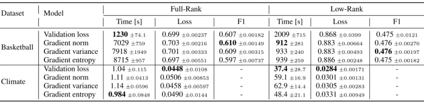
MRTLis not specific to ALS and allows for any other CP decomposition method, such as multiplicative updates for nonnegative CP decomposition. While we can use tensor nuclear norm regularization (Friedland & Lim,2018), this method was computationally infeasible for our datasets. When to finegrain There is a tradeoff between training times at different resolutions. While training for longer at lower resolutions decreases computation significantly, we do not want to overfit to the lower resolution data. On the other hand, training at higher resolutions can yield more accurate solutions using more finegrained information. We investigate four different criteria to balance this tradeoff: 1) validation loss, 2) gradient norm, 3) gradient variance, and 4) gradient entropy.
Increase in validation loss (Prechelt,1998;Yao et al.,2007) is a commonly used heuristic for early stopping. Another approach is to analyze the gradient distributions during train-ing. For a convex functionf, stochastic gradient descent will converge into a noise ball near the optimal solution as the gradients approach zero. However, lower resolutions may be too coarse to learn more finegrained curvatures and the gradients will increasingly disagree near the optimal solution. We quantify the disagreement in the gradients with metrics such as norm, variance, and entropy. We use intuition from convergence analysis for gradient norm and variance (Bottou et al.,2018), and information theory for gradient entropy (Srinivas et al.,2012).
Letwtandξtrepresent the weights and the random
sam-pling of minibatches at stept, respectively. Letf(wt;ξt) :=
ftbe the validation loss andg(wt;ξt) :=gtbe the
stochas-tic gradients at stept. The finegraining criteria are: • Validation Loss:E[ft+1]−E[ft]>0
• Gradient Norm:E[kgt+1k2]−E[kgtk2]>0 • Gradient Variance:V(E[gt+1])−V(E[gt])>0 • Gradient Entropy:S(E[gt+1])−S(E[gt])>0
whereS(p) =P
i−piln(pi). One can also use thresholds,
i.e. |ft+1 −ft| < τ, but as these are dependent on the
dataset, we useτ = 0in our experiments. One can also incorporate patience, i.e. setting the maximum number of epochs where the stopping conditions was reached.
How to finegrain We discuss different interpolation schemes for different types of features. Categori-cal/multinomial variables, such as a player’s position on the court, are one-hot encoded or multi-hot encoded onto a discretized grid. Note that as we use higher resolutions, the sum of the input values are still equal across resolutions, P dX (r) :,:,d = P dX (r+1)
:,:,d . As the sum of the features
re-mains the same across resolutions and our tensor models are multilinear, nearest neighbor interpolation should be used in order to produce the same outputs.
Dr X d=1 W:(,r:,d)X:(,r:,d) = Dr+1 X d=1 W:(,r:,d+1)X:(,r:,d+1)
asXi,f,d(r) = 0for cells that do not contain the value. This scheme yields the same outputs and the same loss values across resolutions.
Continuous variables that represent averages over loca-tions, such as sea surface salinity, often have similar val-ues at each finegrained cell at higher resolutions (as the values at coarse resolutions are subsampled or averaged from values at the higher resolution). An example is Lapla-cian/Gaussian pyramids for images (Burt & Adelson,1983). ThenPDr+1 d X (r+1) :,:,d ≈2 2PDr d X (r)
:,:,d, where the
approxi-mation comes from the type of downsampling used. Using a linear interpolation scheme,
Dr X d=1 W:(,r:,d)X:(,r:,d) ≈22 Dr+1 X d=1 W:(,r:,d+1)X:(,r:,d+1)
The weights are divided by the scale factor ofDr+1
Dr to keep the outputs approximately equal. We use bilinear interpola-tion, though any other linear interpolation can be used.
5. Theoretical Analysis.
5.1. Convergence
We prove the convergence rate forMRTLof a single spatial mode. For a loss functionf and stochastic variableξ, the optimization problem is:
w?=argminE[f(w;ξ)] (5)
We defer all proofs to the Appendix. For a fixed-resolution miniSGD algorithm, under common assumptions in conver-gence analysis:
• f isµ- strongly convex,L-smooth
• (unbiased) gradientE[g(wt;ξt)] =Of(wt)givenξ<t
• (variance) for all the w, E[kg(w;ξ)k22] ≤ σ2g +
cgkOf(w)k22
Theorem 5.1. (Bottou et al.,2018) If the step sizeηt ≡
η≤ 1
Lcg, then a fixed resolution solution satisfies
E[kwt+1−w?k22]≤γ t( E[kw0−w?k22)−β] +β where γ = 1−2ηµ, β = ησ 2 g
2µ, and w? is the optimal
solution.
which givesO(1/t) +O(η)convergence.
Denote the number of total iterations for resolutionras tr, and the weights asw(r). We letDrdenote the
num-ber of dimensions at r and we assume a dyadic scaling between resolutions such that Dr+1 = 2Dr. We define
finegraining using an interpolation operator P such that w(0r+1) = Pw(tr)
r as in (Bramble,2019). For the simple case of a 1D spatial grid wherew(tr)has spatial dimension
Dr, P would be of a Toeplitz matrix of dimension2Dr×Dr.
For example, for linear interpolation ofDr= 2,
Pw(r)= 1 2 1 0 2 0 1 1 0 2 " w(1r) w(2r) # = w(1r+1)/2 w(1r+1) w1(r+1)/2 +w(2r+1)/2 w(2r+1)
Any interpolation scheme can be expressed in this form. The convergence of multiresolution learning algorithm de-pends on the following property of spatial data:
Definition 5.2(Spatial Autocorrelation). The difference be-tween the optimal solutions of consecutive resolution is upper bounded by
kw(?r+1)−Pw
(r)
? k ≤
withPbeing the interpolation operator.
Theorem 5.3. If the step sizeηt ≡ η ≤ Lc1g, thenMRTL
solution satisfies E[kw(tr)−w?k22]≤γ t kPk2oprE[kw0−w?k22+O(ηkPkop) whereγ= 1−2ηµ,β = ησ 2 g
2µ , andkPkopis the operator
norm of the interpolation operatorP.
This gives similar convergence rate as the fixed resolution algorithm, with a constant that depends on the operator norm of the interpolation operatorP.
5.2. Computational Complexity
To analyze computational complexity, we resort to fixed point convergence (Hale et al.,2008) and the multi-grid method (St¨uben,2001). Intuitively, as most of the training
iterations are spent on coarser resolutions with fewer number of parameters, multi-resolution learning is more efficient than fixed-resolution training.
Assuming that∇f is Lipschitz continuous, we can view gradient-based optimization as a fixed-point iteration oper-atorFwith a contraction constant ofγ∈(0,1)(note that stochasticgradient descent converges to a noise ball instead of a fixed point):
w←F(w), F :=I−η∇f, kF(w)−F(w0)k ≤γkw−w0k.
Letw(?r)be the optimal estimator at resolutionrandw(r)be
a solution satisfyingkw?(r)−w(r)k ≤/2. The algorithm
terminates when the estimation error reaches C0R
(1−γ)2. The
following lemma describes the computational cost of the fixed-resolutionalgorithm.
Lemma 5.4. Given a fixed point iteration operatorFwith contraction constant ofγ∈(0,1), the computational com-plexity of fixed-resolution training for tensor model of order pand rankKis C=O 1 |logγ|·log 1 (1−γ) · Kp (1−γ)2 . (6) whereis the terminal estimation error.
The next theorem5.5characterizes the computational speed-up gained by multi-resolution learning compared to fixed-resolution learning, with respect to the contraction factorγ and the terminal estimation error.
Theorem 5.5. If the fixed point iteration operator (gradi-ent desc(gradi-ent) has a contraction factor ofγ, multi-resolution learning with the termination criteria of C0r
(1−γ)2 at
resolu-tionris faster than fixed-resolution learning by a factor of log 1
(1−γ), with the terminal estimation error.
Note that the speed-up using multi-resolution learning uses a global convergence criterionfor eachr.
6. Experiments
We applyMRTLto two real-world datasets: basketball track-ing and climate data.
6.1. Datasets
Tensor classification: Basketball tracking We use a large NBA player tracking dataset from (Yue et al.,2014; Zheng et al.,2016) consisting of the coordinates of all play-ers at 25 frames per second, for a total of approximately 6 million frames. The goal is to predict whether a given ball handler will shoot within the next second, given his position on the court and the relative positions of the de-fenders around him. In applying our method, we hope to
obtain common shooting locations on the court and how a defender’s relative position suppresses shot probability.
Figure 2.Left: Discretizing of a continuous-valued position of a player (red) via a spatial grid. Right: sample frame with a ballhandler (red) and defenders (green). Only players close to the ballhandler are used.
We have two spatial modes: the ball handler’s position and the relative defender positions around the ball handler. We instantiate the tensor classification model in Eqn (1) as follows: Yi= D1 r X d1=1 D2 r X d2=1 σ(Wi,d(r)1,d2X (r) i,d1,d2+bi)
wherei∈ {1, . . . , I}is the ballhandler ID,d1indexes the ballhandler’s position on the discretized court of dimension {D1
r}, andd2indexes the relative defender positions around
the ballhandler in a discretized grid of dimension{D2
r}. As
shown in Fig. 2, we orient the defender positions so that the direction from the ballhandler to the basket points up. Yi∈ {0,1}is the binary output equal to1if playerishoots
within the next second.
We use a weighted cross entropy loss (due to imbalanced classes) and nearest neighbor interpolation for finegraining.
Figure 3.Left: precipitation over continental U.S. Right: regions considered in particular.
Tensor regression: Climate Recent research (Li et al., 2016a;b;Zeng et al.,2019) shows that oceanic variables such as sea surface salinity (SSS) and sea surface tempera-ture (SST) are significant predictors of the variability in rain-fall in land-locked locations, such as the U.S. Midwest. We aim to predict the average monthly precipitation variability in U.S Midwest using SSS and SST to identify meaningful
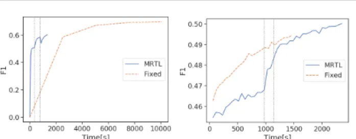
Figure 4.Basketball: F1 scores ofMRTLvs. the fixed-resolution model for the full rank (left) and low rank model (right). The vertical lines indicate finegraining to the next resolution.
latent factors underlying the large-scale processes linking the ocean and precipitation on land (Fig.3)
LetX be the historical oceanic data with input features SSS and SST acrossDrlocations, using the previous6months
of data. We consider the lag as a non-spatial feature so that F1 = 6andF2 = 2as there are two spatial features. We instantiate the tensor regression model in Eqn (1) as follows:
Y = F1 X f1=1 F2 X f2=1 Dr X d=1 Wf(r) 1,f2,dX (r) f1,f2,d+b
We use difference detrending for each timestamp due to non-stationarity of the inputs, and deasonalize by standard-izing each month of the year. The features are normalized using min-max normalization. We also normalize and de-seasonalize the outputs in order to model variability. We use mean square error (MSE) and bilinear interpolation for finegraining.
Implementation Details For both datasets, we discretize the spatial features intoDrcells and use a 60-20-20
train-validation-test set split. We use Adam (Kingma & Ba,2014) for optimization as it was empirically faster than SGD in our experiments. We use bothL2and spatial regularization as described in Section3. We selected optimal hyperparam-eters for all models via random search. We use a stepwise learning rate decay with stepsize of1withγ= 0.95. We perform ten trials for all experiments. All other details are provided in the Appendix.
6.2. Accuracy and Convergence
We compareMRTLagainst a fixed-resolution model on ac-curacy and computation time. The fixed-resolution model uses the same full-rank initialization asMRTLbut utilizes the highest resolution only. The results of all trials are listed in Table1. Other results are provided in the Appendix. Fig. 4shows the F1 scores ofMRTLvs a fixed resolution model for the basketball dataset (validation loss was used as the finegraining criterion for both models). For the full rank case, MRTLconverges 9 times faster than the fixed resolution case. The fixed-resolution model is able to reach
Figure 5.Basketball: F1 scores different finegraining criteria for the full rank (left) and low rank (right) model
a higher F1 score for the full rank case, as it uses a higher resolution and is able to learn more finegrained information. This advantage does not transfer to the low rank model. For the low rank model, the training times are comparable and both reach a similar F1 score. There is decrease in the F1 score going from full rank to low rank for bothMRTL and the fixed resolution model due to approximation error from CP decomposition. Note that this is dependent on the choice ofK, specific to each dataset. We see a similar trend for the climate data, whereMRTLconverges faster than the fixed-resolution model. Overall,MRTLis approximately 4 ∼5 times faster than a fixed-resolution model and we get a similar speedup in the climate data.
6.3. Finegraining Criteria
We compared the performance of different finegraining cri-teria in Fig.5. Validation loss converges much faster than other criteria for the full rank model while the other fine-graining criteria converge slightly faster for the low rank model. In the classification case, we observe that the full rank model spends many epochs training when we use gradient-based criteria, suggesting that they can be too strict for the full rank case. For the regression case, we see all criteria perform similarly for the full rank model, and valida-tion loss converges faster for the low rank model. As there are differences between finegraining criteria for different datasets, one should try all of them for fastest convergence. 6.4. Interpretability
We now demonstrate thatMRTLcan learn semantic repre-sentations along spatial dimensions. For all latent factor figures, the factors have been normalized to(−1,1)so that reds are positive and blues are negative.
Figs.7,8visualize some latent factors for ballhandler po-sition and relative defender popo-sitions, respectively (see Ap-pendix for all latent factors). For the ballhandler position in Fig.7, coherent spatial patterns (can be both red or blue regions as they are simply inverses of each other) can corre-spond to common shooting locations. These latent factors can represent known locations such as the paint or near the three-point line on both sides of the court.
Table 1.Runtime and prediction performance comparison of a fixed-resolution model vsMRTLfor datasets
Dataset Model Full-Rank Low-Rank
Time [s] Loss F1 Time [s] Loss F1
Basketball Fixed 11462±565 0.608±0.00941 0.685±0.00544 2205±841 0.849±0.0230 0.494±0.00417
MRTL 1230±74.1 0.699±0.00237 0.607±0.00182 2009±715 0.868±0.0399 0.475±0.0121
Climate Fixed 12.5±0.0112 0.0882±0.0844 - 269±319 0.0803±0.0861
-MRTL 1.11±0.180 0.0825±0.0856 - 67.1±31.8 0.0409±0.00399
-Figure 6.Climate: Some latent factors of sea surface locations. The red areas in the northwest Atlantic region (east of North America and Gulf of Mexico) represent areas where moisture export contributes to precipitation in the U.S. Midwest.
Figure 7.Basketball: Latent factors heatmaps of ballhandler posi-tion after trainingMRTLfork= 1,3,20. They represent common shooting locations such as the right/left sides of the court, the paint, or near the three point line.
Figure 8.Basketball: Latent factors heatmaps of relative defender positions after trainingMRTLfork = 1,3,20. The green dot represents the ballhandler at(6,2). The latent factors show spatial patterns near the ballhandler, suggesting important positions to suppress shot probability.
For relative defender positions in Fig.8, we see many con-centrated spatial regions near the ballhandler, demonstrating that such close positions suppress shot probability (as ex-pected). Some latent factors exhibit directionality as well, suggesting that guarding one side of the ballhandler may suppress shot probability more than the other side.
Fig.6depicts two latent factors of sea surface locations. We would expect latent factors to correspond to regions of the ocean which independently influence precipitation. The left latent factor highlights the Gulf of Mexico and northwest Atlantic ocean as influential for rainfall in the Midwest, consistent with findings from (Li et al.,2018;2016a).
Random initialization We also perform experiments us-ing a randomly initialized low-rank model in order to verify the importance of full rank initialization. Fig.9compares random initialization vs. MRTLfor the ballhandler posi-tion (left two plots) and the defender posiposi-tions (right two plots). We observe that even with spatial regularization, randomly initialized latent factor models can produce noisy, uninterpretable factors and thus full-rank initialization is essential.
Figure 9.Latent factor comparisons (k= 3,10) of randomly ini-tialized low-rank model (1st and 3rd) andMRTL(2nd and 4th) for ballhandler position (left two plots) and the defender positions (right two plots). Random initialization leads to uninterpretable latent factors.
7. Conclusion and Future Work
We presented a novel algorithm for tensor models for spatial analysis. Our algorithmMRTLutilizes multiple resolutions to significantly decrease training time and incorporates an full-rank initialization strategy that promotes spatially coher-ent and interpretable latcoher-ent factors.MRTLis generalized to both the classification and regression cases. We proved the theoretical convergence of our algorithm for stochastic gradi-ent descgradi-ent and compared the computational complexity of MRTLto a single, fixed-resolution model. The experimental results on two real-world datasets support its computational efficiency and interpretability.
Future work includes 1) develop other stopping criteria in order to enhance the computational speedup, 2) apply our algorithm to more higher-dimensional spatial data, and 3) study the effect of varying batch sizes between resolutions as in (Wu et al.,2019).
References
Anandkumar, A., Ge, R., and Janzamin, M. Guaranteed non-orthogonal tensor decomposition via alternating rank-1 updates. arXiv preprint arXiv:1402.5180, 2014. Austin, W., Ballard, G., and Kolda, T. G. Parallel tensor
compression for large-scale scientific data. InParallel and Distributed Processing Symposium, 2016 IEEE Inter-national, pp. 912–922. IEEE, 2016.
Bahadori, M. T., Yu, Q. R., and Liu, Y. Fast multivariate spatio-temporal analysis via low rank tensor learning. In Advances in neural information processing systems, pp. 3491–3499, 2014.
Bottou, L., Curtis, F. E., and Nocedal, J. Optimization methods for large-scale machine learning. Siam Review, 60(2):223–311, 2018.
Bramble, J. H.Multigrid methods. Routledge, 2019. Brunsdon, C., Fotheringham, S., and Charlton, M.
Geo-graphically weighted regression. Journal of the Royal Statistical Society: Series D (The Statistician), 47(3): 431–443, 1998.
Burt, P. and Adelson, E. The laplacian pyramid as a compact image code.IEEE Transactions on communications, 31 (4):532–540, 1983.
Cheng, H., Yu, Y., Zhang, X., Xing, E., and Schuurmans, D. Scalable and sound low-rank tensor learning. InArtificial Intelligence and Statistics, pp. 1114–1123, 2016. Cressie, N. Statistics for spatial data. Terra Nova, 4(5):
613–617, 1992.
Dieng, A. B., Tran, D., Ranganath, R., Paisley, J., and Blei, D. Variational inference viaχupper bound minimization. InAdvances in Neural Information Processing Systems, pp. 2732–2741, 2017.
Diggle, P. J., Moraga, P., Rowlingson, B., and Taylor, B. M. Spatial and spatio-temporal log-gaussian cox processes: extending the geostatistical paradigm.Statistical Science, pp. 542–563, 2013.
Ding, Y., Kondor, R., and Eskreis-Winkler, J. Multiresolu-tion kernel approximaMultiresolu-tion for gaussian process regression. InAdvances in Neural Information Processing Systems, pp. 3743–3751, 2017.
Doshi-Velez, F. and Kim, B. Towards a rigorous sci-ence of interpretable machine learning. arXiv preprint arXiv:1702.08608, 2017.
Friedland, S. and Lim, L.-H. Nuclear norm of higher-order tensors. Mathematics of Computation, 87(311):1255– 1281, 2018.
Getis, A. and Ord, J. K. The analysis of spatial association by use of distance statistics.Geographical analysis, 24 (3):189–206, 1992.
Hale, E. T., Yin, W., and Zhang, Y. Fixed-point continua-tion for`1-minimization: Methodology and convergence. SIAM Journal on Optimization, 19(3):1107–1130, 2008. Han, S. and Dunson, D. B. Multiresolution tensor decom-position for multiple spatial passing networks. arXiv preprint arXiv:1803.01203, 2018.
Haupt, J., Li, X., and Woodruff, D. P. Near optimal sketch-ing of low-rank tensor regression. InProceedings of the 31st International Conference on Neural Information Pro-cessing Systems, pp. 3469–3479. Curran Associates Inc., 2017.
Hiptmair, R. Multigrid method for maxwell’s equations. SIAM Journal on Numerical Analysis, 36(1):204–225, 1998.
Hitchcock, F. L. The expression of a tensor or a polyadic as a sum of products.Journal of Mathematics and Physics, 6(1-4):164–189, 1927.
Kingma, D. P. and Ba, J. Adam: A method for stochastic optimization. arXiv preprint arXiv:1412.6980, 2014. Kolda, T. G. and Bader, B. W. Tensor Decompositions and
Applications.SIAM Review, 51(3):455–500, 2009. ISSN 0036-1445. doi: 10.1137/07070111X.
Kondor, R., Teneva, N., and Garg, V. Multiresolution matrix factorization. InProceedings of the 31st International Conference on Machine Learning (ICML-14), pp. 1620– 1628, 2014.
Kossaifi, J., Panagakis, Y., Anandkumar, A., and Pantic, M. Tensorly: Tensor learning in python. The Journal of Machine Learning Research, 20(1):925–930, 2019. Lee, D. D. and Seung, H. S. Algorithms for non-negative
matrix factorization. InAdvances in neural information processing systems, pp. 556–562, 2001.
Li, J., Choi, J., Perros, I., Sun, J., and Vuduc, R. Model-driven sparse cp decomposition for higher-order ten-sors. In2017 IEEE international parallel and distributed processing symposium (IPDPS), pp. 1048–1057. IEEE, 2017a.
Li, L., Schmitt, R., Ummenhofer, C., and Karnauskas, K. Im-plications of north atlantic sea surface salinity for summer precipitation over the us midwest: Mechanisms and pre-dictive value. Journal of Climate, 29:3143–3159, 2016a. Li, L., Schmitt, R., Ummenhofer, C., and Karnauskas, K. North atlantic salinity as a predictor of sahel rainfall. Science Advances, 29:3143–3159, 2016b.
Li, L., Schmitt, R. W., and Ummenhofer, C. C. The role of the subtropical north atlantic water cycle in recent us extreme precipitation events. Climate dynamics, 50(3-4): 1291–1305, 2018.
Li, X., Haupt, J., and Woodruff, D. Near optimal sketching of low-rank tensor regression. InAdvances in Neural In-formation Processing Systems 30, pp. 3466–3476, 2017b. Lipton, Z. C. The mythos of model interpretability. Queue,
16(3):31–57, 2018.
Litvinenko, A., Keyes, D., Khoromskaia, V., Khoromskij, B. N., and Matthies, H. G. Tucker tensor analysis of mat´ern functions in spatial statistics. Computational Methods in Applied Mathematics, 19(1):101–122, 2019. Lotte, F. and Guan, C. Regularizing common spatial
pat-terns to improve bci designs: unified theory and new algorithms.IEEE Transactions on biomedical Engineer-ing, 58(2):355–362, 2010.
Miller, A., Bornn, L., Adams, R., and Goldsberry, K. Fac-torized point process intensities: A spatial analysis of professional basketball. InInternational Conference on Machine Learning (ICML), 2014.
Molnar, C. Interpretable machine learning. Lulu. com, 2019.
Moran, P. A. Notes on continuous stochastic phenomena. Biometrika, pp. 17–23, 1950.
Nash, S. G. A multigrid approach to discretized optimization problems.Optimization Methods and Software, 14(1-2): 99–116, 2000.
Ozdemir, A., Iwen, M. A., and Aviyente, S. Multi-scale analysis for higher-order tensors. arXiv preprint arXiv:1704.08578, 2017.
Prechelt, L. Automatic early stopping using cross validation: quantifying the criteria.Neural Networks, 11(4):761–767, 1998.
Reed, S., Oord, A., Kalchbrenner, N., Colmenarejo, S. G., Wang, Z., Chen, Y., Belov, D., and Freitas, N. Parallel multiscale autoregressive density estimation. In Interna-tional Conference on Machine Learning, pp. 2912–2921, 2017.
Ribeiro, M. T., Singh, S., and Guestrin, C. Why should i trust you?: Explaining the predictions of any classifier. pp. 1135–1144, 2016.
Romera-Paredes, B., Aung, H., Bianchi-Berthouze, N., and Pontil, M. Multilinear multitask learning. InInternational Conference on Machine Learning, pp. 1444–1452, 2013. Schifanella, C., Candan, K. S., and Sapino, M. L. Mul-tiresolution tensor decompositions with mode hierarchies. ACM Transactions on Knowledge Discovery from Data (TKDD), 8(2):10, 2014.
Serban, I. V., Klinger, T., Tesauro, G., Talamadupula, K., Zhou, B., Bengio, Y., and Courville, A. C. Multiresolu-tion recurrent neural networks: An applicaMultiresolu-tion to dialogue response generation. InAAAI, pp. 3288–3294, 2017. Sidiropoulos, N. D., De Lathauwer, L., Fu, X., Huang, K.,
Papalexakis, E. E., and Faloutsos, C. Tensor decomposi-tion for signal processing and machine learning. IEEE Transactions on Signal Processing, 65(13):3551–3582, 2017.
Srinivas, N., Krause, A., Kakade, S. M., and Seeger, M. W. Information-theoretic regret bounds for gaussian process optimization in the bandit setting.IEEE Transactions on Information Theory, 58(5):3250–3265, 2012.
St¨uben, K. A review of algebraic multigrid. InPartial Differential Equations, pp. 281–309. Elsevier, 2001. Trottenberg, U., Oosterlee, C. W., and Schuller, A.
Multi-grid. Elsevier, 2000.
Wang, Y., Tung, H.-Y., Smola, A. J., and Anandkumar, A. Fast and guaranteed tensor decomposition via sketching. InAdvances in Neural Information Processing Systems, pp. 991–999, 2015.
Wu, C.-Y., Girshick, R., He, K., Feichtenhofer, C., and Krhenbhl, P. A multigrid method for efficiently training video models, 2019.
Yao, Y., Rosasco, L., and Caponnetto, A. On early stopping in gradient descent learning.Constructive Approximation, 26(2):289–315, 2007.
Yu, R., Li, G., and Liu, Y. Tensor regression meets gaussian processes. In21st International Conference on Artificial Intelligence and Statistics (AISTATS 2018), 2018. Yue, Y., Lucey, P., Carr, P., Bialkowski, A., and Matthews,
I. Learning Fine-Grained Spatial Models for Dynamic Sports Play Prediction. InIEEE International Conference on Data Mining (ICDM), 2014.
Zeng, L., Schmitt, R., Li, L., Wang, Q., and Wang, D. Forecast of summer precipitation in the yangtze river valley based on south china sea springtime sea surface salinity.Climate Dynamics, 53:54955509, 2019. Zheng, S., Yue, Y., and Hobbs, J. Generating long-term
tra-jectories using deep hierarchical networks. InAdvances in Neural Information Processing Systems, pp. 1543–1551, 2016.
Zhou, H., Li, L., and Zhu, H. Tensor regression with applica-tions in neuroimaging data analysis. Journal of the Amer-ican Statistical Association, 108(502):540–552, 2013.
A. Appendix
A.1. Convergence Analysis
Theorem A.1. (Bottou et al.,2018) If the step sizeηt≡η ≤Lc1g, then a fixed resolution solution satisfies
E[kwt+1−w?k22]≤γ t[ E[kw0−w?k22]−β] +β whereγ= 1−2ηµ,β= ησ 2 g
2µ, andw?is the optimal solution.
Proof. For a single step update,
kwt+1−w?k22=kwt−ηtg(wt;ξt)−w?k22
=kwt−w?k22+kηtg(wt;ξt)k22−2ηtg(wt;ξt)(wt−w?) (7)
by the law of total expectation
E[g(xt;ξt)(wt−w?)] =E[E[g(wt;ξt)(wt−w?)|ξ<t]]
=E[(wt−w?)E[g(wt;ξt)|ξ<t]]
=E[(wt−w?)>Of(wt)] (8)
From strong convexity,
hOf(wt)−Of(w?),wt−w?i=hOf(wt),wt−w?i ≥µkwt−w?k22 (9) which impliesE[(wt−w?)>Of(wt)]≥µE[kwt−w?k22]asOf(w?) = 0. Putting it all together yields
E[kwt+1−w?k22]≤(1−2ηtµ)E[kwt−w?k22] + (ηtσg)2 (10)
Asηt=η, we complete the contraction, by settingβ= (ησg)
2
(2ηµ)
E[kwt+1−w?k22]−β≤(1−2ηtµ)(E[kwt−w?k22]−β) (11)
Repeat the iterations
E[kwt+1−w?k22]−β≤(1−2ηµ)
t(
E[kw0−w?k22]−β) (12)
Rearranging the terms, we get
E[kwt+1−w?k22]≤(1−2ηµ)
t
E[kw0−w?]−((1−2ηµ)t+ 1)
(ησg)2
(2ηµ) (13)
Theorem A.2. If the step sizeηt≡η≤ Lc1g, thenMRTLsolution satisfies
E[kw(tr)−w ?k2 2]≤γ t(kPk2 op) r[ E[kw(1)0 −w (1),?k2 2] −γtkPk22β+γ t2(kPk2 opβ−β) +O(1) whereγ= 1−2ηµ,β= ησ 2 g
2µ, andkPkopis the operator norm of the interpolation operatorP.
Consider a two resolution case whereR= 2andw(2)? =w?. Lettrbe the total number of iterations of resolutionr. Based
on Eqn. (10), for a fixed resolution algorithm, aftert1+t2number of iterations,
E[kwt1+t2−w?k
2
2]−β ≤(1−2ηµ)
t1+t2(
For multi-resolution, where we train on resolutionr= 1first, we have E[kwt(1) 1 −w (1) ? k22]−β ≤(1−2ηµ) t1( E[kw(1)0 −w (1) ? k22]−β) At resolutionr= 2, we have E[kw(2)t2 −w?k 2 2]−β ≤(1−2ηµ) t2( E[kw(2)0 −w?k22]−β) (14)
Using interpolation, we havew0(2)=Pw(1)t1 . Given the spatial autocorrelation assumption, we have
kw(2)? −Pw
(1)
? k2≤ By the definition of operator norm and triangle inequality,
E[kw0(2)−w (2) ? k22≤E[kPw (1) t1 −w (2) ? k22]≤ kPk 2 opE[kw (1) t1 −w (1) ? k22] + 2
Combined with eq. (14), we have
E[kw(2)t2 −w?k 2 2]−β≤(1−2ηµ)t2(kPk2opE[kw (1) t1 −w (1) ? k22] +2−β) (15) =(1−2ηµ)t1+t2kPk2 op(E[kw (1) 0 −w (1) ? k22]−β) + (1−2ηµ) t2(kPk2 opβ+ 2−β) (16)
If we initializew0andw(1)0 such thatkw(1)0 −w(1)? k22=kw0−w?k22, we haveMRTLsolution
E[kw 0 t1+t2−w?k 2 2]−α≤(1−2ηµ) t1+t2kPk2 op(E[kw 0 0−w?k22]−α) (17)
for someαthat completes the contraction. Repeat the resolution iterates in Eqn. (16), we reach our conclusion. A.2. Computational Complexity Analysis
In this section, we analyze the computational complexity forMRTL(Algorithm1). Assuming that∇fis Lipschitz continuous, we can view gradient-based optimization as a fixed-point iteration operatorF with a contraction constant ofγ∈(0,1)(note thatstochasticgradient descent converges to a noise ball instead of a fixed point).
w←F(w), F:=I−η∇f,kF(w)−F(w0)k ≤γkw−w0k.
Letw(?r)be the optimal estimator at resolutionr. Suppose for each resolutionr, we use the following fine-grain criterion:
kw(tr)−wt(−r)1k ≤ C0Dr
γ(1−γ). (18)
wheretris the number of iterations taken at levelr. The algorithm terminates when the estimation error reaches (1C−0γR)2.
The following main theorem characterizes the speed-up gained by multi-resolution learningMRTLw.r.t. the contraction factorγand the terminal estimation error.
Theorem A.3. Suppose the fixed point iteration operator (gradient descent) for the optimization algorithm has a contraction factor (Lipschitz constant) ofγ, the multi-resolution learning procedure is faster than that of the fixed resolution algorithm by a factor oflog(1−1γ), withas the terminal estimation error.
We prove several useful Lemmas before proving the main TheoremA.3. The following lemma analyzes the computational cost of thefixed-resolutionalgorithm.
Lemma A.4. Given a fixed point iteration operator with a contraction factor γ, the computational complexity of a fixed-resolution training for ap-order tensor with rankKis
C=O 1 |logγ|·log 1 (1−γ)· Kp (1−γ)2 . (19)
Proof. At a high level, we can prove this by choosing a small enough resolutionrsuch that the approximation error is bounded with a fixed number of iterations. Letw?(r)be the optimal estimate at resolutionrandwtbe the estimate at stept.
Then kw?−wtk ≤ kw?−w (r) ? k+kw (r) ? −wtk ≤. (20)
We pick a fixed resolutionrsmall enough such that
kw?−w
(r)
? k ≤
2, (21)
then using the termination criteriakw?−w
(r)
? k ≤ (1C−0γR)2 givesDr= Ω((1−γ)2)whereDris the discretization size at
resolutionr. Initializew0= 0and applyFtowforttimes such that γt 2(1−γ)kF(w0)k ≤ 2. (22) Asw0= 0,kF(w0)k ≤2C, we obtain that t≤ 1 |logγ|·log 2C (1−γ), (23)
Note that for an orderptensor with rankK, the computational complexity of every iteration inMRTLisO(Kp/Dr)with
Dras the discretization size. Hence, the computational complexity of the fixed resolution training is
C=O 1 |logγ|·log 1 (1−γ)· Kp Dr =O 1 |logγ|·log 1 (1−γ)· Kp (1−γ)2 .
Given a spatial discretizationr, we can construct an operatorFrthat learns discretized tensor weights. The next lemma
relates the estimation error with resolution. The following lemma relates the estimation error with resolution:
Lemma A.5. (Nash,2000) For each resolution levelr= 1,· · ·, R, there exists a constantC1andC2, such that the fixed point iteration with discretization sizeDrhas an estimation error:
kF(w)−F(r)(w)k ≤(C1+γC2kwk)Dr (24)
Proof. See (Nash,2000) for details.
We have obtained the discretization error for the fixed point operation at any resolution. Next we analyze the number of iterationstrneeded at each resolutionrbefore finegraining.
Lemma A.6. For every resolutionr= 1, . . . , R, there exists a constantC0such that the number of iterationstrbefore
finegraining satisfies:
tr≤C0/log|γ| (25)
Proof. According to the fixed point iteration definition, we have for each resolutionr: kFr(wtr)−w (r) tr )k ≤ γ tr−1kF r(w (r) 0 )−w (r) 0 k (26) ≤ γtr−1C0Dr 1−γ (27) ≤ C0γtr−1 (28)
using the definition of the finegrain criterion.
By combining LemmasA.6and the computational cost per iteration, we can compute the total computational cost for our MRTLalgorithm, which is proportional to the total number of iterations for all resolutions:
CMRTL=O 1 |logγ| (Dr/Kp)−1+ (2Dr/Kp)−1+ (4Dr/Kp)−1+· · · =O 1 |logγ| Kp Dr 1 +1 2 + 1 4 +· · · =O 1 |logγ| Kp Dr 1−(1 2) n 1−1 2 =O 1 |logγ| Kp (1−γ)2 , (29)
where the last step uses the termination criterion in (18). Comparing with the complexity analysis for the fixed resolution algorithm in LemmaA.4, we complete the proof.
B. Experiments
Basketball We list implementation details for the basketball dataset. We focus only on half-court possessions, where all players have crossed into the half court as in (Yue et al.,2014). The ball must also be inside the court and be within a 4 feet radius of the ballhandler. We discard any passing/turnover events and do not consider frames with free throws.
For the ball handler location{D1
r}, we discretize the half-court into resolutions4×5,8×10,20×25,40×50. For the
relative defender locations, at the full resolution, we choose a12×12grid around the ball handler where the ball handler is located at(6,2)(more space in front of the ball handler than behind him/her). We also consider a smaller grid around the ball handler for the defender locations, assuming that defenders that are far away from the ball handler do not influence shooting probability. We use6×6,12×12for defender positions.
Let us denote the pair of resolutions as(Dr1, Dr2). We train the full-rank model at resolutions(4×5,6×6),(8×10,6× 6),(8×10,12×12)and the low-rank model at resolutions(8×10,12×12),(20×25,12×12),(40×50,12×12). There is a notable class imbalance in labels (88% of data points have zero labels) so we use weighted cross entropy loss using the inverse of class counts as weights. For the low-rank model, we use tensor rankK= 20. The performance trend of MRTLis similar across a variety of tensor ranks.Kshould be chosen in appropriately to the desired level of approximation.
Climate We describe the data sources used for climate. The precipitation data comes from the PRISM group, which provides estimates monthly estimates at 1/24 spatial resolution across the continental U.S from 1895 to 2018. For oceanic data we use the EN4 reanalysis product, which provides monthly estimates for ocean salinity and temperature at 1 spatial resolution across the globe from 1900 to the present (see Fig.3). We constrain our spatial analysis to the range [-180W, 0W] and [-20S, 60N], which encapsulates the area around North America and a large portion of South America.
The ocean data is non-stationary, with the variance of the data increasing over time. This is likely due to improvement in observational measurements of ocean temperature and salinity over time, which reduce the amount of interpolation needed to generate an estimate for a given month. After detrending and deseasonalizing, we split the train, validation, and test sets using random consecutive sequences so that their samples come from a similar distribution.
We train the full-rank model at resolutions4×9and8×18and the low-rank model at resolutions8×18,12×27,24×54, 40×90,60×135, and80×180. For finegraining criteria, we use a patience factor of 4, i.e. training was terminated when a finegraining criterion was reached a total of 4 times. Both validation loss and gradient statistics were relatively noisy during training (possibly due to a small number of samples), leading to early termination without the patience factor.
During fine-graining, the weights were upsampled to the higher resolution using bilinear interpolation and then scaled by the ratio of the number of inputs for the higher resolution to the number of inputs for the lower resolution (as described in Section4) to preserve the magnitude of the prediction.
Details We trained the basketball dataset on 4 RTX 2080 Ti GPUs, while the climate dataset experiments were performed on a separate workstation with 1 RTX 2080 Ti GPU. The computation times of the fixed-resolution andMRTLmodel were compared on the same setup for all experiments.
B.1. Hyperparameters
Hyperparameter Basketball Climate
Batch size 32−256 8−128
Full-rank learning rateη 10−3−10−1 10−4−10−1
Full-rank regularizationλ 10−5−100 10−4−10−1
Low-rank learning rateη 10−5−10−1 10−4−10−1
Low-rank regularizationλ 10−5−100 10−4−10−1
Spatial regularizationσ 0.03−0.2 0.03−0.2 Learning rate decayγ 0.7−0.95 0.7−0.95
Table 2.Search range forOpthyperparameters
Table2show the search ranges of all hyperparameters considered. We performed separate random searches over this search space forMRTL, fixed-resolution model, and the randomly initialized low-rank model. We also separate the learning rateη and regularization coefficientλbetween the full-rank and low-rank models.
B.2. Accuracy and Convergence
Figure 10.Basketball: Loss curves ofMRTLvs. the fixed-resolution model for the full rank (left) and low rank model (right). The vertical lines indicate finegraining to the next resolution.
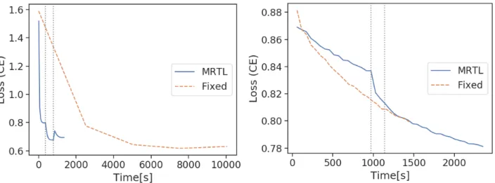
Fig. 10shows the loss curves ofMRTLvs. the fixed resolution model for the full rank and low rank case. They show a similar convergence trend, where the fixed-resolution model is much slower thanMRTL.
B.3. Finegraining Criteria
Table3lists the results for the different finegraining criteria. In the classification case, we see that validation loss reaches much faster convergence than other gradient-based criteria in the full-rank case, while the gradient-based criteria are faster for the low-rank model. All criteria can reach similar F1 scores. For the regression case, all stopping criteria converge to a similar loss in roughly the same amount of time for the full-rank model. For the low-rank model, validation loss appears to converge more quickly and to a lower loss value. Thus one should try all of the finegraining criteria in order to reach the fastest convergence.
Table 3.Runtime and prediction performance comparison of different finegraining criteria
Dataset Model Full-Rank Low-Rank
Time [s] Loss F1 Time [s] Loss F1
Basketball Validation loss 1230±74.1 0.699±0.00237 0.607±0.00182 2009±715 0.868±0.0399 0.475±0.0121 Gradient norm 7029±759 0.703±0.00216 0.610±0.00149 912±281 0.883±0.00664 0.476±0.00270 Gradient variance 7918±1949 0.701±0.00333 0.609±0.00315 933±240 0.883±0.00493 0.476±0.00197 Gradient entropy 8715±957 0.697±0.00551 0.597±0.00737 939±259 0.886±0.00248 0.475±0.00182 Climate Validation loss 1.04±0.115 0.0448±0.0108 - 37.4±28.7 0.0284±0.00171 -Gradient norm 1.11±0.0413 0.0506±0.00853 - 59.1±16.9 0.0301±0.00131 -Gradient variance 1.14±0.0596 0.0458±0.00597 - 62.9±14.4 0.0305±0.00283 -Gradient entropy 0.984±0.0848 0.0490±0.0144 - 48.4±21.1 0.0331±0.00949 -B.4. Random initialization
Fig.11shows all latent factors after trainingMRTLvs a randomly initialized low-rank model for ballhandler position. We can see clearly that full-rank initialization produces spatially coherent factors while random initialization can produce some uninterpretable factors (e.g. the latent factors fork= 3,4,5,7,19,20are not semantically meaningful). Fig. 12shows latent factors for the defender position spatial mode, and we can draw similar conclusions about random initialization.
Figure 11.Basketball: Latent factors of ball handler position after trainingMRTL(left) and a low-rank model using random initialization (right). The factors have been normalized to (-1,1) so that reds are positive and blues are negative. The latent factors are numbered left to right, top to bottom.
Figure 12.Basketball: Latent factors of relative defender positions after trainingMRTL(left) and a low-rank model using random initialization (right). The factors have been normalized to (-1,1) so that reds are positive and blues are negative. The green dot represents the ballhandler at (6, 2). The latent factors are numbered left to right, top to bottom.