A MACHINE LEARNING APPROACH TO WEAK GRID IDENTIFICATION FOR LARGE SCALE ELECTRICAL POWER SYSTEMS
A Thesis by
ANGELICA CLARK
Submitted to the Office of Graduate and Professional Studies of Texas A&M University
in partial fulfillment of the requirements for the degree of MASTER OF SCIENCE
Chair of Committee, Le Xie
Committee Members, Prasad Enjeti Scott Miller Duncan Walker Head of Department, Miroslav M. Begovic
December 2017
Major Subject: Electrical Engineering
ii ABSTRACT
This research proposes a weak grid detection method that is a steady state screening method to identify clusters of buses where potential coordinated voltage oscillations could occur. The objectives of this method are to identify any potential weak grid areas in transmission planning cases with future projected renewable energy under a planning horizon. So that necessary improvements such as transmission projects, voltage support devices or conventional generation are identified for the scenarios in the cases that are being studied. Furthermore, after the necessary improvements have been
identified and made, the change in system strength can be quantified. The benefit of this method is that it is a steady state screening method and does not require computationally and manually intensive dynamic simulations. Several different scenarios in the form of cases can quickly be analyzed, with the resulting areas identified and quantified in each scenario. The contribution of this method is that it is robust and can be applied to any large scale electrical power system under varying operating conditions.
In the proposed method, a random forest algorithm is used to cluster the buses into the weak grid areas based on features extracted from the short circuit current and electrical distance. This method was applied to the ERCOT Current Trends Long Term System Assessment (LTSA) Transmission Planning Case for the year 2031 to
benchmark the capability of the tool and see if it could identify predicted weak grid areas. It was also applied to a transmission planning case representing a Synthetic Texas Network. To demonstrate the robustness of the tool and ability to identify weak grid
iii
areas under different operating conditions and for different systems. The system conditions that were studied in the 2031 ERCOT Current Trends Long Term System Assessment (LTSA) Transmission Planning Case that was analyzed do not reflect actual ERCOT operating conditions. The conclusions in this thesis are only the author’s
iv DEDICATION
v
ACKNOWLEDGEMENTS
I would like to thank my advisor Dr. Xie as well as Dr. Enjeti, both of whom gave me invaluable guidance while I was at Texas A&M University. I’d also like to thank Fred Huang, Yang Zhang and Jose Conto at ERCOT for their technical expertise. Lastly, I’d like to thank my parents and boyfriend for their constant support.
vi
CONTRIBUTORS AND FUNDING SOURCES Contributors
This work was supervised by a thesis committee consisting of Professor Xie, Professor Miller, and Professor Enjeti of the Department of Electrical Engineering and Professor Walker of Computer Science and Engineering. The data analyzed for Chapter 4 was two transmission planning cases. The first case was provided by ERCOT. The second was provided by Dr. Overbye and the Electrical Grid Test Case Repository at Texas A&M University. All work for the thesis was completed independently by the student.
Funding Sources
Graduate study was supported by the Texas A&M Department of Electrical Engineering Graduate Merit Scholarship, the Delbert A. Whitaker Graduate fellowship and the Gulf Coast Power Association Dave Olver Memorial Scholarship.
vii
NOMENCLATURE
ERCOT Electric Reliability Council of Texas
LTSA Long Term System Assessment
SCR Short Circuit Ratio
WSCR Weighted Short Circuit Ratio
POI Point of Interconnection
viii TABLE OF CONTENTS Page ABSTRACT………...ii DEDICATION ... iv ACKNOWLEDGEMENTS ... v
CONTRIBUTORS AND FUNDING SOURCES ... vi
NOMENCLATURE ...vii
TABLE OF CONTENTS ... viii
LIST OF FIGURES ... x
LIST OF TABLES ... xi
CHAPTER I INTRODUCTION ... 1
Weak Bus ... 1
Weak Grid Area ... 4
CHAPTER II LITERATURE REVIEW ... 9
CHAPTER III METHODS ... 11
Short Circuit Current Based Approach ... 11
Tool Algorithm ... 12
Random Forest Classifier ... 14
Random Forest Features ... 15
CHAPTER IV RESULTS ... 19
Performance of Random Forest Model ... 19
2016 ERCOT LTSA ... 20
Case Upgrades ... 25
Synthetic Texas Network ... 28
Sensitivity Analysis ... 33
ix
x
LIST OF FIGURES
FIGURE Page
1.1 Weak Bus Example………. 2
1.2 Example 6 Bus Weak System………. 4
3.1 Example Transmission Pathway………. 16
4.1 Average GINI Feature Importance (K=5) ………. 20
4.2 345 KV ERCOT Short Circuit Heat Map with Clusters……… 22
4.3 138 KV ERCOT Short Circuit Heat Map with Clusters……… 24
4.4 Synthetic Texas Network Map with 500 KV Clusters……….. 29
4.5 Synthetic Texas Network Map with 230 KV Clusters……….. 30
4.6 Synthetic Texas Network Map with 161 KV Clusters……….. 31
xi
LIST OF TABLES
TABLE Page
1.1 SCR Calculation of Sample 6 Bus System………. 8
4.1 345 KV Identified Weak Grid Areas……….. 22
4.2 138 KV Identified Weak Grid Areas……….. 24
4.3 Panhandle Case Upgrade Scenarios……….. 26
4.4 West Case Upgrade Scenarios……….……….. 27
4.5 South Texas Case Upgrade Scenarios……...……… 28
4.6 230 KV Identified Weak Grid Areas……...………. 30
4.7 115 KV Identified Weak Grid Areas……...………. 32
4.8 Voltage Sensitivity of Cluster 2 (115 KV)……...………..…. 33
4.9 Voltage Sensitivity of Cluster 1 (230 KV)……...………..…. 34
1 CHAPTER I INTRODUCTION
The amount of renewable energy in the form of wind and solar generation continues to grow at a significant rate in Texas and in the United States [1,2]. This can be attributed to several factors such as growing concern for the environment and
subsequent interest in clean energy, state and federal incentives as well as the decreasing cost of renewable technology. According to the 2015 Renewable Energy Data Book, 64% of the new installed generation capacity within the United States was from renewable energy [3]. Specifically, an additional 5,600 MW of solar and 8,100 MW of wind was installed in 2015 [3]. Within Texas the amount of installed wind generation is projected to increase from 15,764 MW to 26,248 MW from the year 2015 to 2017 [1]. For solar generation, the installed capacity is expected to increase from 288 MW to 2,057 MW from the year 2015 to 2017 [1]. These trends illustrate that the capacity of renewable generation in Texas and in the United States will only continue to grow and at an increasing rate.
Weak Bus
It is therefore becoming increasingly important to understand the impact that power electronics based renewable forms of generation have on the security and stability of the electrical grid. Renewable, power electronics based technology does not respond well to small fluctuations in voltage. This is because the power converters that interface renewable resources to the electrical grid have dynamic reactive capability meaning they
2
can instantaneously inject or absorb reactive power [4]. This is problematic considering renewable resources are often interconnected at weak buses in resource dense areas that are far from conventional generation. Eqn. (1.1) shows that a large electrical distance to a strong bus will result in a low short circuit current, and that the two parameters are inversely proportional.
𝐼𝑠𝑐 =𝑉
𝑋 (1.1)
To demonstrate, an example of a weak bus that has power electronics based renewable generation, connected to a strong bus is shown in Fig. 1.1 below. The weak bus (Bus 1) is connected to the strong bus (Bus 2), that can regulate its voltage at 1 per unit, over a large electrical distance X12. Eqns. (1.2-1.6) show the calculation for the
voltage sensitivity of the weak bus example.
3 𝑄12 = (𝑉2− 𝐸 ∗ 𝑉𝑐𝑜𝑠𝛿) 𝑋12 (1.2) 𝑑𝑄 𝑑𝑉 = (2𝑉 − 𝐸𝑐𝑜𝑠𝛿) 𝑋12 (1.3) 𝑑𝑄 𝑑𝑉 = (2𝑉 − 𝑐𝑜𝑠𝛿) 𝑋12 , 𝐴𝑠𝑠𝑢𝑚𝑒 𝐸 = 1 𝑝. 𝑢 (1.4) 𝑑𝑉 𝑑𝑄= 𝑋12 (2𝑉 − 𝑐𝑜𝑠𝛿), 𝐴𝑠𝑠𝑢𝑚𝑒 𝐸 = 1 𝑝. 𝑢. (1.5) 𝑑𝑉 𝑑𝑄= 𝑋12 (2𝑉 − 1) , 𝐴𝑠𝑠𝑢𝑚𝑒 𝛿 ≈ 0 (1.6)
The equation for the voltage sensitivity, Eqn. (1.6), shows that if the electrical distance to a strong bus is high, a bus will have a high voltage sensitivity. Meaning that a small change in reactive power will cause a large change in voltage [5].
Connecting power electronics based resources that can dynamically provide reactive power to buses with a high voltage sensitivity can therefore lead to instability. For example, if a change in voltage and subsequent power factor is sensed at the weak bus with a high voltage sensitivity in Fig. 1.1 the resource will respond by quickly injecting reactive power. Due to the high voltage sensitivity to reactive power (dV/dQ), the voltage at the bus will increase significantly. Sensing this increase in voltage and change in power factor, the resource will quickly absorb reactive power leading to a
4
large decrease in voltage. This will continue as the controller of the power electronics based resource struggles to maintain its voltage and can lead to potential sustained, undamped voltage oscillations at a single bus.
Weak Grid Area
Renewable generation is often clustered together in resource dense areas to maximize the generation output. These units can be far from load centers and
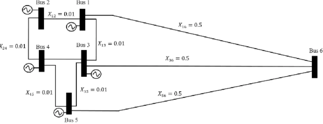
conventional generation. Meaning that the point of interconnection (POI) buses of the renewable units can have a small electrical distance between one another and a large electrical distance from a strong bus, that could aid in regulating its voltage. Because of the small electrical distance between the renewable POI buses, the voltages of the buses are strongly coupled to one another. A small 6 bus system is shown in Fig. 1.2 that illustrates this system topology.
Figure 1.2: Example 6 Bus Weak System
5
In Fig. 1.2 shown above, Buses 1-5 are POI buses with renewable generation and have a small electrical distance between each other. Bus 6 in this example system is the strong bus that can regulate its voltage at 1 per unit. As seen, there is a large electrical distance between the POI buses with renewable generation and the strong bus. As such, the voltages of Buses 1-5 will be coupled to one another. This type of system topology can lead to coordinated, undamped voltage oscillations between multiple renewable POI buses.
At a weak bus such as Bus 1, that is far from conventional generation and a strong bus, if a converter senses a decrease in voltage and corresponding change in power factor. The power electronics converter at Bus 1 will react by suddenly injecting reactive power at the bus [4]. Given that it is a weak bus, it will have a high voltage sensitivity or high dV/dQ value so it will respond with a large increase in voltage. Sensing this large increase in voltage at Bus 1, there will be a sudden absorption of reactive power leading to a large decrease in voltage at Bus 1. The converter at Bus 1 will struggle to maintain its voltage level and the result will be sustained voltage
oscillations at the single bus. However, because Bus 1 has a close electrical distance to Buses 2-5 the voltage oscillations it experiences will have a subsequent effect on that portion of the system.
Buses 2 and 3 are the neighboring buses to Bus 1 and have a small electrical distance so their voltages are tethered to one another. So, as the voltage oscillations occur at Bus 1 the voltages at Buses 2 and 3 will increase and decrease, following the original voltage oscillations at Bus 1. The converter at Bus 2 for example will sense this
6
increase and decrease in voltage as it follows the voltage at Bus 1. Following an increase in voltage, its converter will instantaneously absorb reactive power which will lead to a large decrease in voltage because it also is a weak bus with a high voltage sensitivity. However, while the voltage at Bus 2 decreases due to the absorption it will also remain coupled to the voltage at Bus 1 where its converter is trying to regulate its own voltage. This is also experienced at Bus 3, as all three buses struggle to regulate their own voltages to their desired setpoints while simultaneously being coupled to buses that are also experiencing voltage oscillations. As voltage oscillations occur at Buses 2 and 3, this can lead to voltage oscillations at Buses 4 and 5 as they are coupled to Buses 2 and 3 and their converters struggle to regulate their voltage setpoints. The potential result is that coordinated voltage oscillations can occur between Buses 1-5 and because there is a large electrical distance to the strong bus at Bus 6, it does not aid in regulating the voltage at the renewable POI buses.
To determine the strength of an individual POI bus, the short circuit current ratio (SCR) is the accepted industry standard metric and is shown in Eqn. (1.7) below [6]. PRMW represents the amount of renewable MW that are attributed to that POI bus. If the
SCR of a single bus is less than 3 it is considered to be a weak bus [6].
𝑆𝐶𝑅( 𝑆ℎ𝑜𝑟𝑡 𝐶𝑖𝑟𝑐𝑢𝑖𝑡 𝑅𝑎𝑡𝑖𝑜) =𝑆𝑆𝐶𝑀𝑉𝐴 𝑃𝑅𝑀𝑊
7
The Short Circuit MVA or SCMVA is calculated by applying a three-phase fault to find the short circuit current at the bus and then performing the calculation shown below in Eqn. (1.8).
𝑆ℎ𝑜𝑟𝑡 𝐶𝑖𝑟𝑐𝑢𝑖𝑡 𝑀𝑉𝐴 (𝑆𝐶𝑀𝑉𝐴) = √3 ∗ 𝑉𝐼𝑠𝑐
(1.8)
However, the SCR only indicates the stability of a single bus and its potential to experience voltage oscillations. Alternatively, the Weighted Short Circuit Ratio or WSCR utilized by ERCOT is used to quantify the strength of a cluster of buses and its potential to experience coordinated voltage oscillations [7]. The equation for WSCR is shown in Eqn. 1.9 below [7].
𝑊𝑒𝑖𝑔ℎ𝑡𝑒𝑑 𝑆ℎ𝑜𝑟𝑡 𝐶𝑖𝑟𝑐𝑢𝑖𝑡 𝑅𝑎𝑡𝑖𝑜 (𝑊𝑆𝐶𝑅) = ∑ 𝑆𝑆𝐶𝑀𝑉𝐴𝑖∗ 𝑃𝑅𝑀𝑊𝑖
𝑛 𝑖
(∑ 𝑃𝑛𝑖 𝑅𝑀𝑊𝑖)2 (1.9)
A single bus can have a high SCR value indicating that it is stable. However, it can still be within a cluster of buses whose overall WSCR is low, indicating that
coordinated voltage oscillations can occur. Therefore, solely using the SCR metric is not a good approximation of system strength for a potential weak grid area. This is
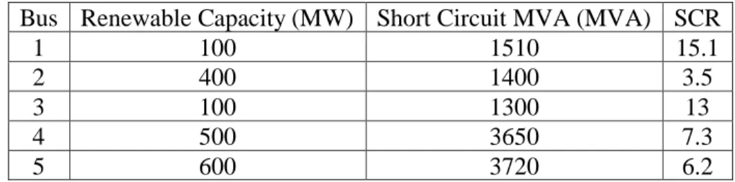
highlighted in the example calculation of the WSCR for the 6 Bus System shown in Fig. 1.2 [7].
8
Bus Renewable Capacity (MW) Short Circuit MVA (MVA) SCR
1 100 1510 15.1
2 400 1400 3.5
3 100 1300 13
4 500 3650 7.3
5 600 3720 6.2
Table 1.1: SCR Calculation of Sample 6 Bus System
𝑊𝑆𝐶𝑅 =∑ 𝑆𝑆𝐶𝑀𝑉𝐴𝑖∗ 𝑃𝑅𝑀𝑊𝑖 𝑛 𝑖 (∑ 𝑃𝑛𝑖 𝑅𝑀𝑊𝑖)2 = (1510 ∗ 100 + 1400 ∗ 400 + 1300 ∗ 100 + 3650 ∗ 500 + 3720 ∗ 600) (100 + 400 + 100 + 500 + 600)2 = 1.69 (1.10) The clustered group of weak buses that was identified for the sample 6 Bus system shown in Fig. 1.2 were Buses 1-5. Looking at Table 1.1, the SCR of each individual bus is greater than 3 indicating that they are not individually weak buses. However, after calculating the WSCR of the identified cluster of weak buses its value was 1.69. Demonstrating that it is a weak grid area where coordinated voltage
oscillations have the potential to occur.
The Panhandle area in the ERCOT system has a system topology containing characteristics similar to the 6 Bus example that were illustrated in Fig. 1.2. There is a significant amount of wind generation in a resource dense area, a large electrical distance to a strong bus and buses in the area have a high voltage sensitivity or dV/dQ value [7]. By performing dynamic simulations, ERCOT simulated that coordinated voltage oscillations occurred between 5 Panhandle POI buses when the WSCR of the identified Panhandle cluster was 1.06 [7]. After inserting synchronous condensers, the new WSCR Panhandle was 1.5 and no coordinated oscillations occurred for the simulation, validating the use of the WSCR metric [7].
9 CHAPTER II LITERATURE REVIEW
This thesis proposes a method to identify weak grid areas where coordinated voltage oscillations can occur within a cluster of buses. It is straightforward to identify individual weak POI buses with renewable generation. Finding the short circuit current or SCR at the POI bus, indicates the potential for sustained voltage oscillations to occur. However, it is a much more rigorous process to identify groups of buses where
coordinated voltage oscillations can occur.
It is challenging to accurately identify clusters of buses for varying types of system topologies. Even more so, to develop a method that is robust enough, it can be applied to different large scale electrical power systems e.g. (ERCOT, CA ISO, MISO, WEC). The proposed method seeks to address these challenges by identifying groups of buses that are coupled together utilizing a machine learning algorithm based on features extracted from the electrical distance and short circuit current.
Network partitioning is a well-researched area in power systems and is related to clustering of power systems. However, much of the focus of this work has been on partitioning large power systems into zones for real time operations applications [8, 9]. The research performed in [8] partitions up generators and load buses that are highly coupled to reduce the computational burden to perform dynamic simulations. In [9] the authors employ a Fuzzy partitioning algorithm to maximize the efficiency of phasor measurement units (PMUs). This thesis diverges from other work as it seeks to identify
10
clustered weak grid areas under a planning horizon. Also, in [10] the network is partitioned using multiple metrics derived from the electrical distance for transmission planning applications and identifying areas with synchronous reserves. The disadvantage of using electrical distance to cluster areas is that the identified areas will solely be based on system topology. Meaning that the results cannot account for different operating conditions. There is a distinct advantage of using a short circuit current based approach, that is used in this thesis, opposed to an electrical distance approach. The short circuit current represents the electrical distance to a strong bus as well as accounts for proximity to nearby resources such as conventional generation. Additionally, its value is based on the operating conditions of the transmission planning case and is not a static metric such as electrical distance.
There has been work done to identify weak buses in a renewable integrated power system [11,12]. In [11] for a test system with integrated wind energy, the authors identify individual weak buses, to determine where additional reactive support is needed and calculate the increased wind transfer capability. In [12] multiple metrics are used to quantify the strength of an individual bus in an integrated wind system. However, these approaches identify single, weak individual buses and don’t consider the coordinated voltage oscillations that can occur when renewable resources are highly coupled.
11 CHAPTER III
METHODS
Short Circuit Current Based Approach
For the purposes of this research, the short circuit current was used to determine the strength of an individual bus. As previously discussed, the advantage of a short circuit current based approach is it accounts for specific operating conditions such as generator status or transmission line outages. Eqn. (1.1) shows that the short circuit current at a bus indicates its electrical distance to a strong bus, as the two parameters are inversely
proportional. For example, if a renewable POI bus has a small electrical distance to a strong bus then it will have a high short circuit current. Whereas a weak bus will have a large electrical distance to a strong bus and will have a low short circuit current value. In addition to considering the electrical distance to a strong bus, it also accounts for
proximity to nearby conventional resources. As the short circuit current of a renewable POI bus will be higher if it is close to a synchronous generator that can contribute supplemental amounts of short circuit current.
Power electronics based resources such as renewable generation have the potential to cause voltage stability issues when they are connected at weak buses with a high dV/dQ metric. To briefly summarize the discussion in Chapter 1. This is because interconnecting power electronic resources with dynamic reactive capability at weak buses can lead to large changes in voltage and potentially, sustained voltage oscillations.
12
The large change in voltage is due to the dynamic absorption and injection of reactive power at buses with a high dV/dQ metric.
Comparing (Eqn. 1.1) and (Eqn. 1.6) that are shown again below. For a weak bus, a high dV/dQ metric also indicates a low short circuit current.
𝐼𝑠𝑐 = 𝑉 𝑋 (1.1) 𝑑𝑉 𝑑𝑄= 𝑋12 (2𝑉 − 1) , 𝐴𝑠𝑠𝑢𝑚𝑒 𝛿 ≈ 0 (1.6)
So therefore, the short circuit current is used as an approximation to estimate the voltage sensitivity at a bus. The approach used for this research to identify weak grid areas was to cluster together buses in the system that had similar voltage sensitivities i.e. short circuit current values. That would have a similar voltage response to a small disturbance and could potentially have coordinated voltage oscillations among the buses in an identified “weak grid” area.
Tool Algorithm
The algorithm for the tool that was created in the programming language Python [13,14,15] was used to identify weak grid areas in PSS/E transmission planning cases and is described below in sequential order:
1. Case Preparation Step: Prepare the case by modifying certain case conditions to study specific operating points.
13
2. Calculate System Wide Short Circuit Current: Calculate the short circuit current of every electrical bus in the entire system by applying a 3-phase fault at that bus.
3. Determine Weak Renewable POI Buses: Use the short circuit current to gauge the strength of an individual renewable POI bus. Based on if the short circuit current for a renewable POI bus is below a percentile threshold (user input) for its corresponding voltage level then it is considered to be weak.
4. Find all Unique Transmission Pathways for Weak POI Buses: For every weak renewable POI bus (step 3), every unique transmission pathway was found n (user input) levels away. Transmission pathways were only found at discrete voltage levels, for the voltage level of the original renewable POI bus. The short circuit current was determined for every bus along the transmission pathway as well as the electrical distance between buses. 5. Random Forest Algorithm: A random forest algorithm was used to
determine when a transition occurred from a weak to a strong bus along a transmission pathway from the original POI bus. The random forest algorithm is explained in further detail below.
6. Identify Individual Clusters: All the buses identified before a detected transition from step 5, are included in the cluster for the original weak POI bus.
14
7. Determine Unique Clusters: A smart sorting method was used to identify if individual clusters were unique or needed to be combined, and is explained in further detail below.
8. Calculate WSCR of distinct clusters: Based on the unique clusters that were identified in Step 7, the WSCR was calculated for every unique cluster.
9. Identify Potential Weak Grid Regions: The calculations from step 8 are used to identify potential weak grid regions where a unique cluster with a WSCR less than 3 was considered weak.
Random Forest Classifier
A random forest classifier is a type of decision classifier tree. A decision classifier tree is a decision tree that is created based on features of its data set [16]. The classifier tree can have binary or linear split points that determine the path an instance will follow, according to its feature value. The final leaves are the endings points of the decision tree and determine what the value of the classifier is. A random forest model is a form of supervised learning, meaning that it trains on data where the value of the classifier has already been defined [17]. Unlike a traditional classifier decision tree that is a single tree, a random forest generates multiple trees that are a combination of the defined features of the data set. Each generated tree predicts the final value of the classifier, and the results from each generated tree are aggregated to produce the final classifier result. An advantage of random forest classifiers over single decision trees is that applications have been shown to be more accurate [18]. Additionally, it is less likely
15
that overfitting will occur for a random forest model. Overfitting occurs when the model has been overfitted to its training data, meaning that it correctly predicts the results for the data it was trained on. However, it cannot accurately predict the results for the testing portion of the data set or new unlabeled data [19]. Because the results of the random forest are aggregated decisions based on multiple trees whereas a classifier decision tree is the result of a single tree, it is inherently less prone to overfitting. Lastly, the benefit of the random forest model is that it does not require significant tuning of model
parameters. Whereas the accuracy of a classifier decision tree is highly dependent on the structure of the tree for the accuracy of the classifier results. Properly tuning a classifier tree is highly dependent on specific knowledge of the data as well as its features. For this application, one objective of this research is to create an algorithm that is robust enough it can be applied on large electrical power systems where significant knowledge of that system is not required.
Random Forest Features
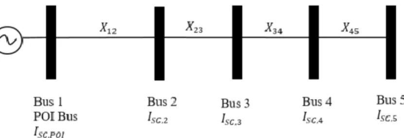
A popular application of the random forest model is in biology, where it is utilized to analyze a significant number of samples for peak detection [20]. For this research, the random forest model is applied to detect a step change in system strength from a bus to the next proceeding bus along a transmission pathway. A test system is shown below for illustration in Fig. 3.1. The features that were used for this research are described below and pertain to the two-bus segment, between Bus 2 and Bus 3.
16
Figure 3.1: Example Transmission Pathway
1. Range of Short Circuit Current: The short circuit current of a bus subtracted by the short circuit current of the preceding bus along the transmission pathway.
𝐼𝑟𝑎𝑛𝑔𝑒 = 𝐼𝑠𝑐,3− 𝐼𝑠𝑐,2 (3.1)
2. Inflection Point: Indicates if an inflection point occurs between two buses, for the curve that is fit to the short circuit current along the transmission pathway. For example, if there was an inflection point in between Bus 2 and Bus 3, the feature value would be 1 otherwise it would be 0.
3. Normalized Range of Short Circuit Current: The range of the normalized short circuit current. When the short circuit current values along the transmission pathway are normalized by the POI bus short circuit current value.
𝐼𝑛𝑜𝑟𝑎𝑚𝑙𝑖𝑧𝑒𝑑 𝑟𝑎𝑛𝑔𝑒 =𝐼𝑠𝑐,3 𝐼𝑃𝑂𝐼 −
𝐼𝑠𝑐,2
17
4. Standard Deviation: The standard deviation of the short circuit current values for all the buses along the transmission pathway.
𝜎 = √ 1 𝑁∑(𝐼𝑆𝐶,𝑃𝑂𝐼− 𝜇) 2 + (𝐼𝑆𝐶,2− 𝜇) 2 + (𝐼𝑆𝐶,3− 𝜇) 2 + (𝐼𝑆𝐶,− 𝜇) 2 + (𝐼𝑆𝐶,5− 𝜇) 2 𝑁 𝑖=1 (3.3)
5. Normalized Standard Deviation: The standard deviation of the short circuit of the segmented two buses divided by the standard deviation of the values for all the buses along the transmission pathway.
𝜎𝑛𝑜𝑟𝑚=
√ 𝑁1∑𝑁 (𝐼𝑆𝐶,2− 𝜇)2+ (𝐼𝑆𝐶,3− 𝜇)2
𝑖=1
𝜎 (3.4)
6. Electrical Distance: The electrical distance between the two segmented buses.
𝑋 = 𝑋23
(3.5) Additionally, a K Fold Cross Validation was performed for 5 K-Folds to
determine if the model was overfitting to the training data. After the individual clusters were formed, a smart sorting method is used to determine if the individual clusters are unique or need to be combined. An initial matrix is formed, using a distance metric
18
(Eqn. 3.6). The distance metric is defined by the number of matching buses between 𝑐𝑙𝑢𝑠𝑡𝑒𝑟 𝑖 and 𝑐𝑙𝑢𝑠𝑡𝑒𝑟 𝑗 divided by the number of buses in 𝑐𝑙𝑢𝑠𝑡𝑒𝑟 𝑖.
𝑑𝑖𝑗 =𝑛𝑢𝑚𝑏𝑒𝑟 𝑜𝑓 𝑚𝑎𝑡𝑐ℎ𝑖𝑛𝑔 𝑏𝑢𝑠𝑒𝑠
𝑏𝑢𝑠𝑒𝑠 𝑖𝑛 𝑐𝑙𝑢𝑠𝑡𝑒𝑟 𝑖 (3.6)
The matrix that is formed is shown below in Eqn. 3.7.
[ 𝑑11 𝑑12 𝑑13 𝑑1𝑁 𝑑21 𝑑22 𝑑23 𝑑2𝑁 𝑑31 𝑑32 𝑑33 𝑑3𝑁 𝑑𝑁1 𝑑𝑁2 𝑑𝑁3 𝑑𝑁𝑁 ] (3.7)
Clusters 𝑖 and 𝑗 will combine if 𝑑𝑖𝑗 or 𝑑𝑗𝑖 are greater than a specified user input. The matrix will reform after clusters have combined and will continue until no value within the matrix is greater than the specified input.
19 CHAPTER IV
RESULTS
Performance of Random Forest Model
To test the performance of the random forest model, 100 random transmission pathways (including roughly 350 transition buses) were labeled. The labeled data specified if a transition occurred between two buses (classifier=1) or if a transition did not occur (classifier=0). K Fold Cross Validation was performed to determine if
overfitting occurred, meaning that the model was trained and tested 5 times [15,16,17]. Performing cross fold validation, it was found that the average percentage accuracy over the 5 folds was 95.4%. Additionally, the percentage accuracy did not significantly change between folds demonstrating that the model was not overfitting.
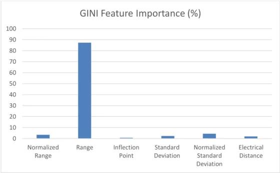
The average GINI importance of each feature was found over 5 folds and is shown below in Fig. 4.1.
20
Figure 4.1: Average GINI Feature Importance (K=5)
Looking at Fig. 4.1, the range is the most important feature and has an average GINI feature importance of 87.3%. A K Fold Cross Validation was performed for a random forest model that only included range as the feature, to determine the accuracy of the model solely based on range. The average accuracy over 5 K Folds for this model was 94.8%. Although that is not significantly lower than the original accuracy of 95.4% when all 6 features were used. All 6 features were used for the final model that was used to analyze the transmission planning cases for this research. As the other features may be utilized when applying the tool on a new large-scale power system, that the user has less prior system knowledge of.
2016 ERCOT LTSA
The first transmission planning case that the tool was applied on was the 2016 ERCOT Current Trends Long Term System Assessment (LTSA) Case for the year 2031
0 10 20 30 40 50 60 70 80 90 100 Normalized Range Range Inflection Point Standard Deviation Normalized Standard Deviation Electrical Distance
21
that has a combined wind and solar capacity of 41,700 MW [21]. The Current Trends LTSA Case represents the forecasted trends for the year 2031. A forecasted trend that is represented in the case, is the significant amount of renewable generation that is present in the Panhandle and West Texas. The Panhandle and Valley area are already recognized as areas of concern. However, the ability to identify the Panhandle area as a weak grid area and properly define its boundary was used to benchmark the capability of the tool. This is because renewable resources in the Panhandle are clustered close together and it is far from conventional generation and load, city centers [7]. Also, the renewable generation in the Panhandle is transmitted over long transmission lines meaning that is a has a large electrical distance to a strong bus. Because it is also far from conventional generation, there is no supplemental fault current being delivered to the renewable POI buses. Also, based on additional renewable capacity being placed in West Texas for the LTSA it is expected that there will be weak grid areas there as well.
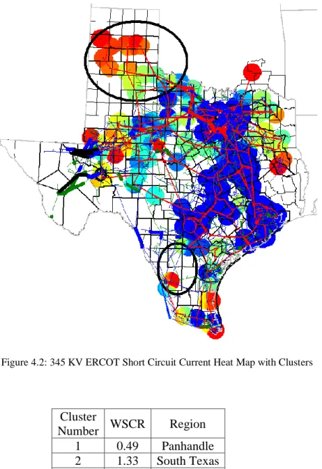
To perform the case preparation step, all the renewable generation was turned off so that it did not provide any contributing short circuit current to renewable POI buses to model the most conservative scenario. Additionally, when calculating the WSCR of each identified unique cluster, the full renewable capacity was used to determine the most conservative WSCR metric. It should be noted that more conservative assumptions are used in this test case and the WSCR metric presented in this thesis doesn’t reflect the actual system constraints. Below in Fig. 4.2 is a short circuit current heat map of the ERCOT system at the 345 KV voltage level, red indicates areas of low short circuit current level compared to relatively high short circuit current level in the blue areas.
22
Additionally, clusters with a WSCR value that are less than 3 are circled on the map in Fig. 4.2. The identified clusters at the 345 KV voltage level are summarized in Table 4.1.
Figure 4.2: 345 KV ERCOT Short Circuit Current Heat Map with Clusters
Cluster
Number WSCR Region 1 0.49 Panhandle 2 1.33 South Texas
3 2.06 West
23
As seen from Table 4.1, three different clusters were identified. Cluster 1, is shown at the top of the map and identifies the Panhandle cluster and its WSCR value is 0.49. The tool was able to identify the Panhandle and draw a precise boundary around the region, demonstrating its capability. Cluster 2 is shown at the bottom of the map and identifies a cluster in South Texas that has a WSCR value of 1.33. Lastly, a very small cluster was identified in the West with a WSCR of 2.06.
This procedure was repeated at the 138 KV level and the short circuit current heat map and identified clusters with a WSCR less than 3 are shown on the map in Fig. 4.3. For the LTSA case, a significant amount of solar generation was added at the 138 KV level and in West Texas so it is expected that weak clusters are identified in the region. The identified clusters with a WSCR less than 3 are shown in Table 4.2.
24
Figure 4.3: 138 KV ERCOT Short Circuit Current Heat Map with Clusters
Cluster
Number WSCR Region
1 1.16 West
2 1.21 West
Table 4.2: 138 KV Identified Weak Grid Areas
There were two clusters identified at the 138 KV level with a WSCR less than 3. Cluster 1 was identified in the West and is the smaller cluster located furthest West on the map shown in Fig 4.3. Its WSCR value is 1.16. Cluster 2 was identified in the West and is the larger cluster that is shown in Fig 4.3, it has a WSCR of 1.21. As expected, weak grid areas were identified in West Texas due to the significant amount of solar
25
generation that is interconnected there. Looking at the short circuit current heat map for the 138 KV level shown in Fig. 4.3 there are a lot of regions that have low short circuit current where there is no cluster identified with a WSCR value less than 3. This means that there is no renewable generation present at a POI in the region or there was a cluster identified in the area, however its WSCR value is greater than 3. For example, for the region below the Panhandle shown in Fig. 4.3 the map indicates that is a region with low short circuit current. However, the cluster that was identified in that area has a WSCR of 4.66.
Case Upgrades
The objective of this tool is to be a steady state screening method to identify weak grid areas where potential control instability or voltage oscillations could occur under specific renewable generation and case scenarios. After identifying the weak grid areas, due to the future projected renewable generation that was present in the ERCOT Current Trends LTSA case for the year 2031. The tool can now be used as a screening method to identify any case improvements such as transmission projects, voltage support devices or conventional generation to determine their effect on the strength of existing weak grid areas. By doing this analysis, the user can study the case improvements that may be required for future projected renewable generation scenarios under specific case conditions.
To illustrate the case improvements that would need to be made to improve the strength of the 345 KV clusters, one upgrade that was considered was synchronous condensers [7]. Synchronous condensers are a type of voltage support device, that
26
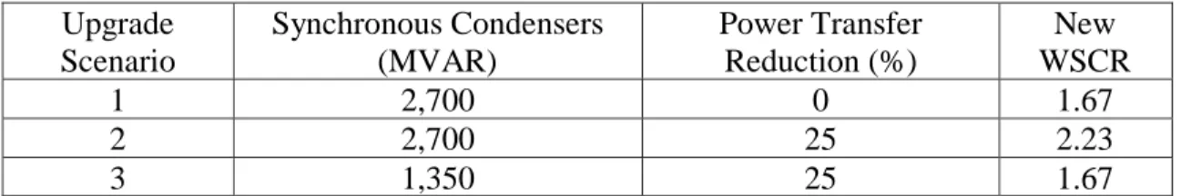
provide reactive power as well as short circuit current. The first cluster that was considered was the Panhandle cluster which had an original WSCR value of 0.49. The considered upgrades were modeled to study the case improvements that would be required to increase the WSCR to a threshold of 1.5 for the conservative case conditions that were studied. This is because ERCOT has established a WSCR threshold of 1.5 for the Panhandle to maintain voltage stability [7]. The proposed system upgrades are summarized in Table 4.3 below.
Upgrade Scenario Synchronous Condensers (MVAR) Power Transfer Reduction (%) New WSCR 1 2,700 0 1.67 2 2,700 25 2.23 3 1,350 25 1.67
Table 4.3: Panhandle Case Upgrade Scenarios
Looking at Table 4.3, under Case Upgrade Scenario 1 a capacity of 2,700 MVAR of synchronous condensers needs to be added to the case to increase the WSCR from 0.49 to 1.67. For Case Upgrade Scenario 2 if the power transfer from the Panhandle is reduced by 25% and a capacity of 2,700 MVAR of synchronous condensers is added to the case, the new WSCR of the cluster is 2.23. Lastly, in the third scenario if the
Panhandle power transfer is reduced by 25% and a capacity of 1,350 MVAR of
synchronous condensers is added to the case then the new WSCR is 1.67. Studying the three scenarios, case upgrade scenario 3 is the most practical approach as it reduces the power transfer from the Panhandle by only 25% and requires 1,350 MVAR of
27
synchronous condensers. So, the final WSCR is 1.67 and greater than the required 1.5 threshold. It should be clarified that the upgrade scenarios that were tested in this case are mainly used to improve system strength. However, a more detailed reliability assessment would be required to ensure transient, voltage stability for the studied case conditions.
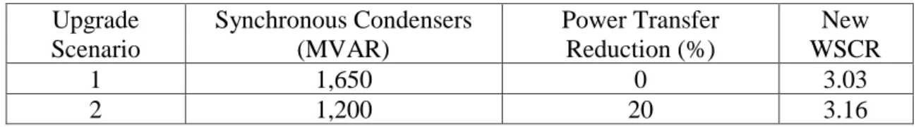
This analysis was also performed on the other 345 KV clusters identified in the ERCOT LTSA Case, the South Texas and West clusters. However, for these clusters the necessary WSCR threshold was 3 rather than the Panhandle threshold of 1.5. This is because the WSCR threshold of 1.5 for the Panhandle was established through dynamic simulations [7]. Applying a threshold requiring the WSCR of the South Texas and West clusters to be greater than 3 for proposed case upgrade scenarios is a more conservative approach. Also, it is extended from the industry standard where the SCR of an individual bus is weak if it less than 3 [6]. Table 4.4 below summarizes the Case Upgrade scenarios for the West Cluster that originally had a WSCR of 1.33.
Upgrade Scenario Synchronous Condensers (MVAR) Power Transfer Reduction (%) New WSCR 1 1,650 0 3.03 2 1,200 20 3.16
Table 4.4: West Case Upgrade Scenarios
Table 4.4 shows that in Case Upgrade Scenario 1 by adding a capacity of 1,650 MVAR of synchronous condensers to the cluster that it increases the WSCR to 3.03. In Scenario
28
2, 1,200 MVAR of synchronous condensers were added and the power transfer from the West Cluster was reduced by 20% increasing the WSCR to 3.16. Analyzing the
proposed case upgrade scenarios, both upgrades present good options.
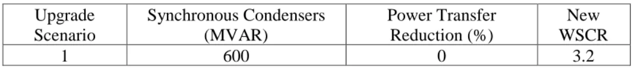
The last cluster that was considered was the cluster in South Texas with an original WSCR of 2.06 and the results are summarized in Table 4.5.
Upgrade Scenario Synchronous Condensers (MVAR) Power Transfer Reduction (%) New WSCR 1 600 0 3.2
Table 4.5: South Texas Case Upgrade Scenario
Only one case upgrade scenario was studied that required a conservative capacity of 600 MVAR and did not require a reduction in power transfer from the South Texas cluster. The WSCR increased from 2.05 to 3.2 after the case changes were made.
Synthetic Texas Network
The tool was also applied on a different case and large-scale power system, a Synthetic Model of the ERCOT system [22]. Although it is a representation of the ERCOT system, it contains a different transmission and generation network. It was used to test the robustness of the tool and asses if it could identify weak grid areas for
different power systems. Based on system knowledge as well as the general areas of concern, the tool should identify areas in the Valley, West Texas and Panhandle region.
29
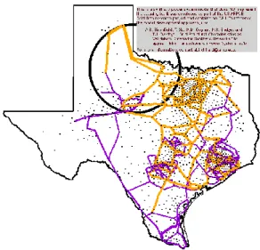
A map showing the Synthetic Texas network is shown below in Fig. 4.4 where the identified weak grid areas less than 5 are circled. Only one cluster was identified with a WSCR less than 5, the cluster in the Panhandle has a WSCR of 4.65.
Figure 4.4: Synthetic Texas Network Map with 500 KV Clusters
Fig. 4.5 shows a map of the Synthetic Texas Network with the clusters identified at the 230 KV level. Table 4.6 summarizes the clusters identified at that voltage level. Two clusters were identified, a large cluster in the West that has a WSCR of 1.95. As well as a smaller cluster in the West that extends into the Panhandle with a WSCR of 4.79.
30
Figure 4.5: Synthetic Texas Network Map with 230 KV Clusters
Cluster Number WSCR Region
1 1.95 West
2 4.79 West
Table 4.6: 230 KV Identified Weak Grid Areas
Fig 4.6 shows a map of the Synthetic Texas Network with clusters identified at the 161 KV level. Only one cluster was identified with a WSCR less than 5, a Panhandle cluster with a WSCR of 2.69.
31
Figure 4.6: Synthetic Texas Network Map with 161 KV Clusters
Lastly, Fig 4.7 shows a map of the clusters identified at the 115 KV level and they are summarized in Table 4.7.
32
Figure 4.7: Synthetic Texas Network Map with 115 KV Clusters
Cluster Number WSCR Region
1 0.44 West 2 0.95 West 3 1.41 West 4 3.03 West 5 3.74 Valley 6 4.91 West
Table 4.7: 115 KV Identified Weak Grid Areas
Cluster 1 has a WSCR of 0.44 and is the large cluster in West Texas that begins at the bottom of the Panhandle and ends at the border of Mexico. Cluster 2 has a WSCR of 0.95 and is a small cluster in West Texas below the Panhandle. Cluster 3 has a WSCR of 1.41 and is in the middle of West Texas. Cluster 4 has a WSCR of 3.03 and is the
33
cluster located on the bottom of West Texas. Cluster 5 has a WSCR of 3.74 and is in the Valley. Lastly, Cluster 6 is a small cluster located at the top of West Texas.
Sensitivity Analysis
To verify the capability of the tool, a voltage sensitivity analysis was performed for three different clusters with a WSCR value less than 3. For each cluster, the voltage sensitivity was found for two POI renewable buses within the cluster by placing a fixed shunt capacitor at the bus and finding the corresponding change in voltage. This same procedure was performed for two buses at the same voltage level in a known strong area, as a point of comparison. If the clustering method properly worked only individual weak buses with a high voltage sensitivity should be within the cluster. Also, their voltage sensitivities should be significantly higher than strong buses at the same corresponding voltage level.
This analysis was first performed on Cluster 2 at the 115 KV level located in West Texas with a WSCR of 0.95 and the results are summarized in Table 4.8.
Bus Voltage Sensitivity (p.u.) Voltage Sensitivity (kV) Region Type
1 0.000619 0.0699 West Weak
2 0.00948 0.0836 West Weak
3 9.252E-05 0.0106 Houston Strong
4 0.000192 0.0220 Houston Strong
Table 4.8: Voltage Sensitivity of Cluster 2 (115 KV)
Looking at Table 4.8, Buses 1 and 2 are the buses that are located within the cluster and Buses 3 and 4 are the strong buses located in Houston. Comparing their
34
voltage sensitivities, the voltage sensitivity values of the buses in Houston are much lower than the weak buses in the West cluster. The second cluster that was analyzed was Cluster 1 at 230 KV, with a WSCR of 1.95 and in West Texas the results are shown in Table 4.9.
Bus Voltage Sensitivity (p.u.) Voltage Sensitivity (kV) Region Type
1 0.000242 0.0561 West Weak
2 6.418-05 0.0148 West Weak
3 2.157E-06 0.000510 Houston Strong
4 1.509E-05 0.00348 Houston Strong
Table 4.9: Voltage Sensitivity of Cluster 1 (230 KV)
Again, the voltage sensitivities of the weak buses in the West cluster, Buses 1 and 2, are significantly higher than the strong buses in Houston, Buses 3 and 4. Lastly, the same analysis was performed for the 161 kV Panhandle cluster with a WSCR of 2.69 and the results are shown in Table 4.10. The voltage sensitivity for the weak buses that are located within the cluster is over ten times higher when compared with the strong buses that are in the Fort Worth area.
35
Bus Voltage Sensitivity (p.u.) Voltage Sensitivity (kV) Region Type
1 0.00149 0.241 Panhandle Weak
2 0.00145 0.231 Panhandle Weak
3 0.000126 0.0203 Fort Worth Strong
4 8.934E-05 0.0144 Fort Worth Strong
Table 4.10: Voltage Sensitivity of Panhandle Cluster (161 KV)
The voltage sensitivity analysis was performed to asses if the tool was able to identify weak grid areas for a new large-scale power system. Specifically, to verify that the voltage sensitivity values of the buses within the identified weak grid areas were significantly higher than buses located in strong areas of the system. The analysis performed on the three clusters above demonstrates that the buses located within the clusters have a much higher sensitivity than the buses in strong areas. Validating the ability of the tool to identify weak grid areas in new large-scale power systems.
36 CHAPTER V CONCLUSIONS
This research proposes a steady state screening method to identify weak grid areas where coordination voltage oscillations could occur within transmission planning cases. The benefit of this method is that the user can identify potential areas of concern under projected renewable generation and specific case conditions. Furthermore,
necessary case upgrades can be identified such as synchronous condensers, transmission expansion and conventional generation that would be required to improve system strength under the studied case conditions.
The tool was applied on the 2016 ERCOT LTSA Current Trends case for the year 2031 to benchmark its capability and asses if it could specifically identify the Panhandle and other known areas of concern. After accurately identifying the Panhandle area as well as other known areas of concern. It was demonstrated how the tool could be utilized as a screening method to identify case upgrades by adding synchronous
condensers to the identified weak grid areas in the Panhandle, South Texas and the West. The method was tested on a second system, a Synthetic ERCOT Network that contained a different transmission and generation network. This was done to
demonstrate if the tool was robust enough to properly identify weak grid areas for a new large-scale power system. A voltage sensitivity analysis was performed on the identified clusters to verify that the clusters were weak grid areas. Doing this analysis, it was
37
shown that the voltage sensitivity within the identified clusters was significantly higher than that at known, strong buses validating the weak grid areas.
Further work that can be performed on this area is rigorous validation of the WSCR metric under different topologies. As well as additional validation of identified weak grid areas using dynamic simulations.
38 REFERENCES
[1] Magness, B. (2016). Future Directions for ERCOT.
[2] Mai, T.; Sandor, D.; Wiser, R.; Schneider, T (2012). Renewable Electricity Futures Study: Executive Summary. NREL/TP-6A20-52409-ES. Golden, CO: National Renewable Energy Laboratory.
[3] Beiter, Philipp, and Tian Tian. “2015 Renewable Energy Data Book,”. U.S.
Department of Energy’s National Renewable Energy Laboratory (NREL)., Golden, CO, 2015.
[4] A. Ellis et al., "Reactive power performance requirements for wind and solar plants," 2012 IEEE Power and Energy Society General Meeting, San Diego, CA, 2012, pp. 1-8.
[5] J. Sun, "Impedance-Based Stability Criterion for Grid-Connected Inverters," in IEEE Transactions on Power Electronics, vol. 26, no. 11, pp. 3075-3078, Nov. 2011. [6] P. Kundur, Power System Stability and Control. New York: McGraw-Hill, 1994. [7] Y. Zhang, S. H. F. Huang, J. Schmall, J. Conto, J. Billo and E. Rehman, "Evaluating system strength for large-scale wind plant integration," 2014 IEEE PES General Meeting Conference & Exposition, National Harbor, MD, 2014, pp. 1-5
[8] S. B. Yusof, G. J. Rogers and R. T. H. Alden, "Slow coherency based network partitioning including load buses," in IEEE Transactions on Power Systems, vol. 8, no. 3, pp. 1375-1382, Aug 1993.
[9] I. Kamwa, A. K. Pradhan, G. Joos and S. R. Samantaray, "Fuzzy Partitioning of a Real Power System for Dynamic Vulnerability Assessment," in IEEE Transactions on Power Systems, vol. 24, no. 3, pp. 1356-1365, Aug. 2009.
[10] E. Cotilla-Sanchez, P. D. H. Hines, C. Barrows, S. Blumsack and M. Patel, "Multi -Attribute Partitioning of Power Networks Based on Electrical Distance," in IEEE Transactions on Power Systems, vol. 28, no. 4, pp. 4979-4987, Nov. 2013.
[11] B. Maya, S. Sreedharan and J. G. Singh, "An integrated approach for the voltage stability enhancement of large wind integrated power systems," 2012 International Conference on Power, Signals, Controls and Computation, Thrissur, Kerala, 2012, pp. 1-6.
39
[12] R. Yajun, Z. Xinhui and N. Huan, "Power system static voltage stability analysis including large-scale wind farms and system weak nodes identification," 2014 International Conference on Power System Technology, Chengdu, 2014, pp. 2747 -2753.
[13] Stéfan van der Walt, S. Chris Colbert and Gaël Varoquaux. The NumPy Array: A Structure for Efficient Numerical Computation, Computing in Science &
Engineering, 13, 22-30 (2011), DOI:10.1109/MCSE.2011.37
[14] Wes McKinney. Data Structures for Statistical Computing in Python, Proceedings of the 9th Python in Science Conference, 51-56 (2010)
[15] Fabian Pedregosa, Gaël Varoquaux, Alexandre Gramfort, Vincent Michel, Bertrand Thirion, Olivier Grisel, Mathieu Blondel, Peter Prettenhofer, Ron Weiss, Vincent Dubourg, Jake Vanderplas, Alexandre Passos, David Cournapeau, Matthieu Brucher, Matthieu Perrot, Édouard Duchesnay. Scikit-learn: Machine Learning in Python, Journal of Machine Learning Research, 12, 2825-2830 (2011)
[16] L. Brieman et. al, Classification and Regression Trees. Belmont, CA. Wadsworth, 1984.
[17] L. Breiman. “Random Forests”, Machine Learning, vol.45 n.1, pp.5-32, Oct. 2001 [18] Tin Kam Ho, "The random subspace method for constructing decision forests," in IEEE Transactions on Pattern Analysis and Machine Intelligence, vol. 20, no. 8, pp. 832-844, Aug 1998.
[19] S. Shalev-Shwartz, S. Ben-David. Understanding Machine Learning: From Theory to Algorithms. New York, NY: Cambridge University Press, 2014.
[20] J. Barret and D. Cairns, “Application of the Random Forest Classification Method to Peaks Detected from Mass Spectrometric Proteomic Profiles of Cancer Patients and Controls,” Statistical Applications in Genetics and Molecular Biology, vol. 7, no. 2, 2008.
[21] S. Borkar et al., “2016 Long-Term System Assessment for the ERCOT
Region,”ERCOT, Taylor, TX, Dec, 2016.
[22] A. B. Birchfield, T. Xu, K. M. Gegner, K. S. Shetye and T. J. Overbye, "Grid Structural Characteristics as Validation Criteria for Synthetic Networks," in IEEE Transactions on Power Systems, vol. 32, no. 4, pp. 3258-3265, July 2017.