Approximate Parallel High Utility Itemset Mining

(1)

APPROXIMATE PARALLEL HIGH UTILITY ITEMSET MINING

YAN CHEN

A THESIS SUBMITTED TO

THE FACULTY OF GRADUATE STUDIES

IN PARTIAL FULFILMENT OF THE REQUIREMENTS FOR THE DEGREE OF

MASTER OF SCIENCE

GRADUATE PROGRAM IN COMPUTER SCIENCE YORK UNIVERSITY

TORONTO, ONTARIO OCTOBER 2015

R

(2)

Abstract

High utility itemset mining discovers itemsets whose utility is above a given thresh-old, where utilities measure the importance of itemsets. In high utility itemset mining, memory and time performance limitations cause scalability issues, when the dataset is very large. In this thesis, the problem is addressed by proposing a distributed parallel algorithm,PHUI-Miner, and a sampling strategy, which can be used either separately or simultaneously. PHUI-Minerparallelizes the state-of-the-art high utility itemset mining algorithmHUI-Miner. The sampling strategy inves-tigates the required sample size of a dataset, in order to achieve a given accuracy. We also propose an approach combining sampling with PHUI-Miner, which pro-vides better time performance. In our experiments, we show thatPHUI-Miner has high performance and outperforms the state-of-the-art non-parallel algorithm. The sampling strategy achieves accuracies much higher than the guarantee. Extensive experiments are also conducted to compare the time performance of PHUI-Miner with and without sampling.

(3)

Acknowledgements

I would like to express my sincere gratitude to my supervisor, Prof. Aijun An, for her valuable guidance throughought my entire period of research. Her advice and support are greatly appreciated. I am also truly grateful to my committee member, Prof. Jarek Gryz, for reviewing my research and providing me his advice.

Numerous individuals provided support in different ways, which enabled me to complete this research. Special thanks to Hanwei Jin, who helped me gain the authorization to use a cluster of computers in Zhejiang University in my early stage of research. Thanks to my labmate, Morteza Zihayat, from whom I learned a lot including essential research and writing skills. I am grateful to my friends, Jing Zhang and Heidar Davoudi, for their help in solving an issue in this thesis. They both provided me with significant afflatuses. I would also like to thank Ricky Fok and Yingying Zhang for their support.

Financial support from York University is also heartily acknowledged.

(4)

and support. I’m specially thankful to my girlfriend, Yaying Chen, for her patience and encouragement while I took the time to complete my research.

(5)

List of Tables

3.1 An Example Transaction Database with External Utilities . . . 12

3.2 Transaction Weighted Utilities (TWUs) for the Example Database . 14 4.1 Revised Transactions . . . 17

6.1 Parameters of the Synthetic Dataset . . . 51

6.2 Values of Parameters . . . 58

6.3 Statistics of Datasets in the Sampling Strategy . . . 60

6.4 Values of Parameters . . . 60

6.5 Top 10 Frequent Patterns ofglobe . . . 71

(9)

List of Figures

4.1 Initial Utility-Lists . . . 18

4.2 Search Space . . . 19

4.3 Data Flow of PHUI-Miner . . . 21

5.1 Data Flow for Getting Statistics of a Dataset . . . 36

6.1 Running Time of PHUI-Miner on (a) kosarak, (b) accidents, (c) chess, (d) twitter, (e) T5000L10I1P10PL6, (f) ta-feng and (g)globe 58 6.2 Speedup of PHUI-Miner . . . 59

6.3 Sample Size of (a)accidents, (b) T5000L10I1P10PL6and (c) twitter 61 6.4 Sample Sizes for Different Sizes of Datasets . . . 62

6.5 Accuracy of Sampling on (a)accidents, (b)T5000L10I1P10PL6and (c) twitter . . . 64

6.6 Accuracy of Sampling without AFPs on (a)accidents, (b)T5000L10I1P10PL6 and (c)twitter . . . 65

(10)

6.7 Average Value and Standard Deviation of Relative Utility Error on (a) accidents, (b) T5000L10I1P10PL6 and (c)twitter . . . 66

(11)

1 Introduction

Frequent pattern mining has been an important topic since the concept of frequent itemsets was first introduced by Agrawal et al [6]. Given a dataset of transac-tions, frequent pattern mining finds the itemsets whose support (i.e. the percentage of transactions containing the itemset) is no less than a given minimum support threshold. However, neither the number of occurrences of an item in a transaction, nor the importance of an item, is considered in frequent pattern mining. Itemsets with more occurrences or importance may be more interesting to users, since they may bring more profit.

In light of this, high utility itemset mining has been studied [9, 15, 42, 35]. In high utility itemset mining, the term utility refers to the importance of an itemset; e.g., the total profit the itemset brings. An itemset is a High Utility Itemset(HUI) if the utility of the itemset is no less than a given minimum threshold. High utility itemset mining focuses more on the utility values in the dataset, which are usually related to profits for the business. Such utilities are interesting to the business

(12)

owners, who could gain more profits from them. For example, supermarkets use frequent itemset mining to find merchandises customers usually buy together, so as to make recommendations to customers. However, with high utility itemset mining, supermarkets will be able to recommend not only the merchandises people usually buy together, but also the merchandises which will lead to more profits for the store.1

Most of the frequent pattern mining algorithms prune off itemsets in an early stage based on the popular Apriori property [8]: every sub-pattern of a frequent pattern must be frequent (also called the downward closure property). However, this property does not hold in high utility itemset mining, which makes mining high utility itemsets more challenging. The state-of-the-art approaches achieve good performance when the dataset is relatively small. However, the volume of data can grow so faster than expected, that a single machine may not be able to handle a very large amount of data.

One option to solve the problem of large volumes of data is to use parallel distributed computing techniques. The MapReduce framework [18] (e.g., Hadoop) has been a popular solution recently, which enables scalable and fault-tolerant dis-tributed processing of huge data on large clusters. Applications in the MapReduce framework have to conform the protocols of mapper and reducer as a disk-based

1_{In Section 6.3, another example will be given to show a real world application of high utility}

(13)

paradigm, which restricts the flexibility as well as the performance of the algorithm. Spark is also a distributed computing framework, which is memory-based, and thus provides performance up to 100 times faster than Hadoop for certain applications [44]. Spark uses Resilient Distributed Dataset (RDD), which is a distributed mem-ory abstraction, for in-memmem-ory computation of data, allowing efficient reuse of data. For very large datasets, obtaining exact results is sometimes infeasible. Recent studies focus on mining an approximate set of frequent itemsets. In most cases, ap-proximate solutions may already be satisfactory to users. In general, approximation methods can be divided into two categories: pattern compressing [13, 34, 12, 43] andsampling[40, 37, 49, 47]. Sampling is a method that mines approximate results from a sample of the entire dataset. The most important step in sampling is to decide the size of the sample we need in order to obtain a certain accuracy, which is also the focus of our sampling strategy proposed in this thesis.

In this thesis, we address the problem of high utility itemset mining by proposing PHUI-Miner(Parallel High Utility Itemset Miner) and a sampling strategy. PHUI-Miner is a parallel distributed algorithm, which parallelizesHUI-Miner, a state-of-the-art algorithm for high utility itemset mining. The sampling strategy provides the required sample size for a dataset in order to achieve a given accuracy. It can be used together with any exact high utility itemset mining algorithm. To the best of our knowledge, this is the first piece of work to utilize sampling in high utility

(14)

itemset mining. Our contributions are summarized as follows:

• PHUI-Miner, a parallel distributed algorithm, is proposed for parallel mining of high utility itemsets without sampling, which could lead to exact results.

• We propose and prove a new theorem, which shows the relationship between the high utility itemset mining results from the whole dataset, and those from a sample of it. The theorem leads to a sampling method with theoretical guarantees on the probability that an HUI can be returned and on the utility of a returned itemset. A feature of this sampling method is that the sample size required to achieve the theoretical guarantees is independent of the size of the original data, and is thus not necessarily going up as the data set grows.

• We also proposePHUI-Miner with sampling, an approach combining sampling with PHUI-Miner, which mines an approximate set of high utility itemsets, but achieves better performances.

• Extensive experiments are conducted and the time performance and scalabil-ity ofPHUI-Minerare evaluated. PHUI-Mineris demonstrated to outperform the state-of-the-art non-parallel high utility itemset mining algorithm HUI-Miner. The time performance ofPHUI-Miner with samplingis also evaluated, which is shown to be better than using PHUI-Miner alone. Furthermore, the accuracy of the sampling strategy is evaluated with several datasets and

(15)

different parameters. Our results show that our sampling strategy achieves accuracy even higher than the expectations based on our theoretical analysis.

The thesis is organized as follows. Chapter 2 is a literature survey of related work. Chapter 3 introduces relevant definitions and a problem statement. Chapter 4 presents PHUI-Miner. Chapter 5 describes the sampling strategy and PHUI-Miner with sampling. We show experimental results in Chapter 6, and conclude the thesis in Chapter 7.

(16)

2 Related Work

Before the problem of high utility itemset mining was first proposed by Yao et al. [46], a variation of the problem, named share frequent itemsets mining, was studied by many researchers. Several algorithms have been proposed: e.g., ZP [11], ZSP [11], FSH [31], ShFSH [31], and DCG [30]. These algorithms can be used to mine high utility itemsets. However, they all use the Apriori [7] like strategy, which results in the problem of repeated database scans and large numbers of candidates. To improve the performance of these algorithms, Liu et al. proposed Two-phase [36], which uses an important utility measure, namedTransaction Weighted Utility (TWU), for pruning the search space, since the downward closure property is not applicable in high utility itemset mining. Afterwards, another pruning strategy, called the isolated items discarding strategy (IIDS), was proposed in FUM [32] and DCG+ [32]. The number of candidates are largely reduced by these pruning strategies. However, the problem of repeated database scans is still not solved. An algorithms based on FP-Growth algorithm [22] have been proposed to mine

(17)

high utility itemsets with at most three scans of database, and thus have better performance. Examples of these algorithms include IHUP [9], HUC-Prune [10], UP-Growth [42], UP-UP-Growth+ [41]. However, the candidate itemsets are still too many compared to the high utility itemsets. HUI-Miner [35] is one of the recent efficient algorithms proposed by Liu et al. demonstrated to have an order of magnitude better performance than other algorithms.

Parallel distributed algorithms solve the problem of mining massive datasets. Several studies [17, 28, 45, 27, 20, 23] have been done for mining frequent patterns in distributed environments, inspired by the MapReduce framework proposed by Google [18]. Some of them [17, 28, 45] use a naive approach which computes the support of every itemset in the dataset in a single MapReduce round, resulting in huge data replication. An adaption of FP-Growth algorithm to MapReduce, called PFP [27], is a more sophisticated approach. Given a minimum frequency threshold, PFP first applies a parallel and distributed counting approach to compute the frequent items. The frequent items are then partitioned into groups randomly. Subsequently, the dataset is used to generate group-dependent transactions, which are sent to reducers. Finally, the reducers use an FP-Growth like approach to generate group-dependent frequent itemsets. However, very few studies have been conducted on high utility itemset mining with distributed computing techniques so far.

(18)

As the volume of data grows, the mining task consumes more and more time. Mannila et al. [38] first suggested that sampling can be used to efficiently obtain association rules. Then Toivonen [40] presented a sampling algorithm, which builds a complete set of association rules with a probability depending on the sample size. The Chernoff bound and the union bound are used, in which the Bernoulli random variable refers to whether an itemset appears in a transaction. A number of previous works [49, 25, 51, 29, 50, 14, 16] have been focusing on improving the bound of the sample size using different techniques in association rules mining or frequent pattern mining. Sampling techniques in high utility itemset mining are more complicated since an itemset has a utility value in each transaction, instead of 0 or 1 in frequent pattern mining. There has hitherto been little research on using sampling in high utility itemset mining.

(19)

3 Preliminaries

3.1 Distributed Computing Frameworks

In data mining and other fields which require analyzing and extracting information from data, the hardware restricts the size of the data we are able to process. CPU, memory and data storage are three different kinds of resources which affect the overall scalability of algorithms. These resources are limited, so it is very hard to process a very large dataset which usually exceeds the capacity of the resources. Distributed computing frameworks solve this problem by using a cluster of com-puters, connected by a network, to perform computing tasks in parallel.

The most commonly known distributed computing framework is Apache Hadoop [1]. Apache Hadoop provides reliable, scalable, and distributed computing solution, which is used by many companies, including Yahoo! and Facebook.

There are two main parts in the core of Apache Hadoop, the storage part and the processing part. The storage part, also known as Hadoop Distributed File System (HDFS), stores data by splitting them into blocks and distributing them

(20)

amongst different nodes in the cluster. Each block of a file is usually replicated, and stored in several different nodes, so that data loss in HDFS is very rare in case of hardware failure. The processing part, also known as MapReduce, uses two procedures, map and reduce, for parallel processing of data. The map and reduce procedures are called mappers and reducers respectively. In mappers, a set of data is converted into tuples (key-value pairs), while reducers take output from mappers and combine tuples into smaller sets of tuples, by aggregating tuples with the same key into a single tuple. HDFS and MapReduce are inspired by the ideas proposed by Google based on the Google File System (GFS) and their proprietary MapReduce technology.

However, there are some drawbacks of Apache Hadoop, which limits the perfor-mance and flexibility of the algorithms implemented on it. On the one hand, the MapReduce paradigm requires that each mapper is followed by a reducer, and they must be programmed in a strictly pre-defined way. On the other hand, each pair of mapper and reducer in Apache Hadoop has to read data from disks, and write results back to disks, which results in a bottleneck in its performance.

In order to deal with these two drawbacks of Apache Hadoop, another dis-tributed computing framework, Apache Spark, was developed. Instead of the two-stage disk-based MapReduce paradigm introduced in Apache Hadoop, Apache Spark uses a data abstraction, known as Resilient Distributed Datasets (RDD).

(21)

RDDs are read-only, partitioned collection of records, which are created by reading from data storages or transforming from other RDDs. [48] An RDD holds refer-ences to Partition objects, where each Partition object is a subset of the dataset represented by this RDD. RDDs are usually not in materialized form. Instead, if an RDD A is transformed from another RDD B, we only need the information of the transformation and the RDD B, in order to derive the RDD A. As a result, RDDs are only materialized when they are asked to perform a reduce operation, which aggregates data in different nodes to a single machine. Apache Spark loads data into the memories of machines in a cluster as RDDs, and uses them repeatedly for data processing tasks. Apache Spark also allows programmers to have arbitrary mappers and reducers in any order, providing a much more flexible API for its users. In an Apache Spark cluster, there is one M aster node and several W orker

nodes. TheM aster node is responsible for allocating resources and assigning tasks toW orkernodes. However, Apache Spark is only an alternative for MapReduce in Apache Hadoop. HDFS is still a state-of-the-art open source distributed data stor-age framework. Apache Spark has interfaces with different types of data storstor-age, including HDFS, Cassandra [2], OpenStack Swift [3], etc. Apache Spark is able to read from these types of data storage for data processing, which makes Spark more popular. Therefore, in this thesis, Apache Spark is used as the main platform for our proposed algorithms, while HDFS is used as our data storage.

(22)

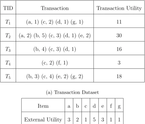
TID Transaction Transaction Utility T1 (a, 1) (c, 2) (d, 1) (g, 1) 11 T2 (a, 2) (b, 5) (c, 3) (d, 1) (e, 2) 30 T3 (b, 4) (c, 3) (d, 1) 16 T4 (c, 2) (f, 1) 3 T5 (b, 3) (c, 4) (e, 2) (g, 2) 18

(a) Transaction Dataset

Item a b c d e f g

External Utility 3 2 1 5 3 1 1

(b) External Utilities

Table 3.1: An Example Transaction Database with External Utilities

3.2 High Utility Itemset Mining

LetI∗ ={I1, I2, ..., Im}be a set of items. An itemsetXis a set of items{Ie1, Ie2, ..., IeZ},

where Z is the length of X, denoted by |X|. A dataset D is a list of transactions {T1, T2, ..., Tn}, where each transaction Td∈D is an itemset.

Definition 1. (Internal utility and external utility) In high utility itemset mining, each itemI ∈I∗ is associated with a positive valuep(I), called its external utility (e.g., item profit). Each itemI in transactionTd∈Dis also associated with

(23)

a positive value q(I, Td), called its internal utility (e.g. purchase quantity). For

example, in Table 3.1,p(b) = 2 and q(b, T2) = 5.

Definition 2. (Utility of an itemI in transaction Td) GivenI ∈Td, the utility

of item I in transaction Td is defined as u(I, Td) = p(I)q(I, Td). For example, in

Table 3.1,u(b, T2) =p(b)q(b, T2) = 10.

Definition 3. (Utility of an itemsetXin transactionTd) The utility of itemset

X in transaction Td is defined as u(X, Td) = P

I∈X

u(I, Td), if X ⊆ Td. Otherwise,

u(X, Td) = 0. For example, in Table 3.1,u({b, c}, T2) = u(b, T2)+u(c, T2) = 10+3 = 13.

Definition 4. (Utility of an itemset X in dataset D) The utility of itemset

X in dataset D is defined as uD(X) = P Td∈D

u(X, Td). For example, in Table 3.1,

uD({b, c}) =u({b, c}, T2) +u({b, c}, T3) +u({b, c}, T5) = 13 + 11 + 10 = 34.

Definition 5. (Utility of a transaction Td) The utility of transaction Td is

defined as u(Td) = P I∈Td

u(I, Td). For example, in Table 3.1, u(T4) = u(c, T4) +

u(f, T4) = 2 + 1 = 3.

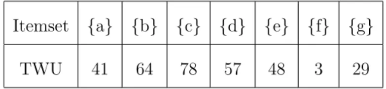
Definition 6. (Transaction weighted utilization of an itemset X in dataset

D) The transaction weighted utilization (TWU) of an itemset X in dataset D is defined as twu(X) = P

X⊆Td,Td∈D

u(Td). For example, in Table 3.1, twu({b, c}) =

(24)

Itemset {a} {b} {c} {d} {e} {f} {g}

TWU 41 64 78 57 48 3 29

Table 3.2: Transaction Weighted Utilities (TWUs) for the Example Database

Transaction weighted utilization has downward closure property, which means for any itemsetX and utility thresholdθ, iftwu(X)< θ, the utility of any superset of X is lower thanθ. For example, since twu({b, c}) = 64, any superset of X will have utility lower than 64. Table 3.2 shows the TWU values for each item in the example database.

Definition 7. (Total utility of a dataset D) The total utility of dataset D is defined as UD = P

Td∈D

u(Td). For example, in Table 3.1, UD =u(T1) +u(T2) +...+

U(T5) = 84.

Definition 8. (Relative utility of an itemset X in a datasetD) The relative utility of an itemsetX in dataset D is defined as uD(X)

UD .

Definition 9. (High utility itemset) An itemsetXis ahigh utility itemset(HUI) in dataset D, iff uD(X) is no less than θUD, where θ is a user specified minimum

relative utility threshold.

Given a datasetDand a user specified minimum relative utility thresholdθ, the problem of high utility itemset mining is to discover all the high utility itemsets in

(25)

D.

However, mining all the high utility itemsets from a very large dataset is very time and memory consuming. Distributed computing framework and sampling based algorithms are, thus, more suitable to this task. In this thesis, distributed computing framework and sampling are both utilized in our proposed algorithms.

(26)

4 PHUI-Miner: Parallel High Utility Itemset

Mining

In this chapter, we propose a parallel high utility itemset mining algorithm, named PHUI-Miner (Parallel High Utility Itemset Miner), which parallelizes the state-of-the-art high utility itemset mining algorithm HUI-Miner [35]. PHUI-Miner is proposed to mine exact results from a dataset, based on Apache Spark. PHUI-Miner adopts a way to split the search space, which is inspired by PFP [27] from Google.

Below, the HUI-Miner algorithm will be reviewed first, so that the reader can better understand our proposed approach. And then, our novel parallel distributed algorithm PHUI-Miner is elaborated.

4.1 Review of HUI-Miner

HUI-Miner mines high utility itemsets without candidate generation. It utilizes a utility-list structure to store the utility information of a database. Constructing

(27)

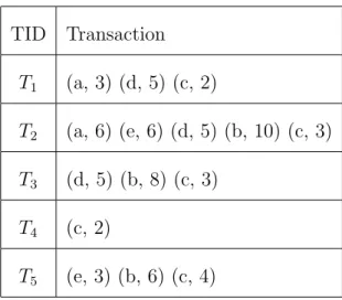
TID Transaction T1 (a, 3) (d, 5) (c, 2) T2 (a, 6) (e, 6) (d, 5) (b, 10) (c, 3) T3 (d, 5) (b, 8) (c, 3) T4 (c, 2) T5 (e, 3) (b, 6) (c, 4)

Table 4.1: Revised Transactions

the initial utility-lists needs two database scans. The first scan of database accu-mulates the TWU values for all the items. During the second database scan, the unpromising items are filtered, and the rest of the items in all the transactions are sorted according to their TWU, in ascending order. The filtered and sorted transactions are called revised transactions. Simultaneously, the initial utility-lists are constructed. The structure of utility-lists is explained later in this section.

For example, in the example database in Table 3.1, if the utility threshold is 30,

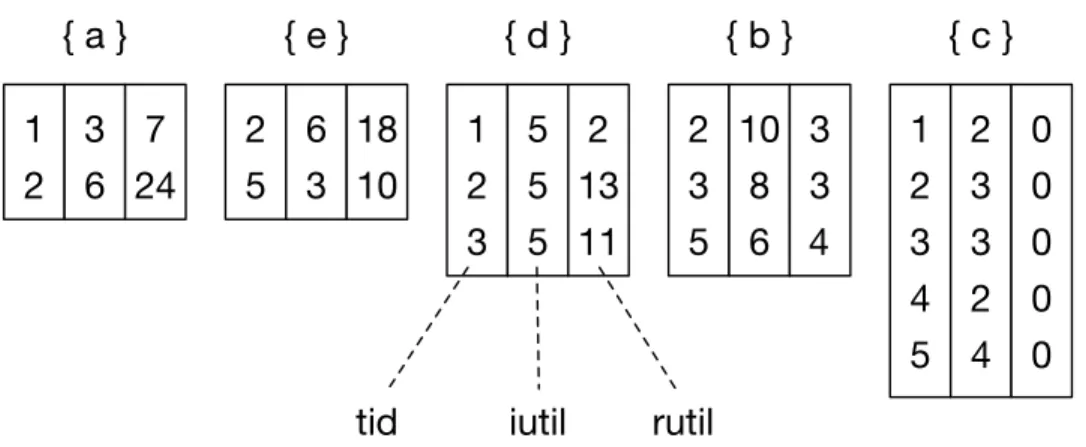
f andg are unpromising items since their TWU values are less than 30. The rest of the items are sorted according to their TWU ascending order: a < e < d < b < c. The revised transactions of the example database are shown in Table 4.1. In the utility-lists, each utility-list of itemsetX has a list of elements, where each element contains three fields: tid,iutil and rutil. [35]

(28)

{ a } 1 2 3 6 7 24 { e } 2 5 6 3 18 10 { d } 1 2 5 5 2 13 { b } 2 3 10 8 3 3 { c } 1 2 2 3 0 0 3 5 11 5 6 4 3 4 5 3 2 4 0 0 0

tid iutil rutil

Figure 4.1: Initial Utility-Lists

• tid is the transaction ID of T containingX. • iutil is the utility of X in T.

• rutilis the sum of utilities of all the items after X in T.

Figure 4.1 shows the initial utility-lists constructed by the second database scan. Then utility-lists of k-itemsets are constructed from utility-lists of (k-1)-itemsets and (k-2)-itemsets recursively. The utility-list of itemset P xy is constructed from utility-lists of itemsets P, P x and P y, where P is an itemset, while x and y are items. For example, to construct the utility-list of itemset edbc, the utility-lists of itemsets ed, edb and edc are needed. In the case of k = 2, the utility-lists of 2-itemsets are constructed from utility-lists of 1-itemsets and itemsets. Since 0-itemsets are empty 0-itemsets, the utility-lists of 0-0-itemsets are defined to be empty too in HUI-Miner. Algorithm 1 [35] shows the procedure in constructing a

(29)

utility-root

a e d _b _c

ae ad ab ac ed eb ec db dc bc

aed aeb aec adb adc abc edb edc ebc dbc

aedb aedc aebc adbc edbc

aedbc

Figure 4.2: Search Space

list of a k-itemset.

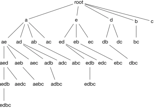
The search space of high utility itemset mining can be represented as a set-enumeration tree [39]. In the tree, each node is an itemset. Given a list of items sorted in their TWU ascending order, the children of the root node is all the items. The other nodes in the tree are generated by appending an item to the itemset

X in the parent node. The item is from the siblings of the parent node whose itemsets are the same asXexcept for the last item. The last items of those siblings are appended to X as the children of the parent node. For example, given five items with TWU ascending order a < e < d < b < c, the set-enumeration tree is

(30)

depicted in Figure 4.2 [35]. HUI-Minermines HUIs recursively, using a depth first search in the search tree. HUI-Miner also prunes subtrees of the search space if it determines that all the itemsets in the subtrees are unpromising based on some criterion. Algorithm 2 [35] shows the procedure ofHUI-Miner.

4.2 PHUI-Miner

PHUI-Miner is a distributed algorithm, which parallelizes HUI-Miner. In PHUI-Miner, the search space is divided and assigned to each node in a cluster. Each node is only responsible for mining the assigned search space, which in another word, splits the workload into different nodes in the cluster.

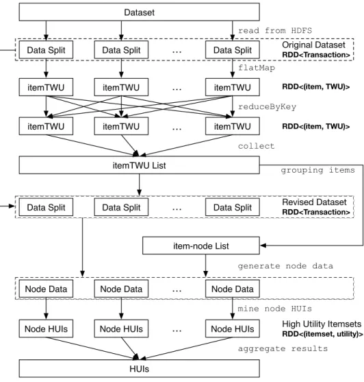
Figure 4.3 is the data flow of PHUI-Miner. Given a transaction dataset D, PHUI-Miner first reads the dataset from HDFS to different nodes. The dataset is stored in HDFS in a distributed way, that the dataset is split into blocks, where every block has a fixed size, defined in the configuration file of HDFS, except the last block. The blocks are usually replicated to ensure reliability. The dataset is read fromHDFS in a unit of block, and the blocks will be as evenly distributed in different nodes as possible. Also, the blocks will be assigned to their local nodes if possible, to lower the communication cost. Each node stores a part of D. Then, itemTWU list is built, which contains the TWU values of each item in the whole dataset. itemTWUis used to revise the transactions, which prunes the unpromising

(31)

Dataset

Data Split Data Split … Data Split

itemTWU itemTWU … itemTWU

itemTWU Original Dataset RDD<Transaction> flatMap reduceByKey itemTWU itemTWU itemTWU List collect RDD<(item, TWU)> RDD<(item, TWU)>

Data Split Data Split … Data Split Revised Dataset

RDD<Transaction> …

read from HDFS

item-node List

Node Data Node Data … Node Data

grouping items

generate node data

Node HUIs Node HUIs … Node HUIs

mine node HUIs

High Utility Itemsets RDD<(itemset, utility)>

HUIs

aggregate results

(32)

items and sorts the items in ascending order according to their TWU values in all the transactions. itemTWUis also used to generate an item-node list, which assigns each promising item to a node in the cluster, as described in Section 4.2.1. The item-node list is also required for generating transactions required for each node to mine their assigned search space, referred to as node data. The details of generating node data are described in Section 4.2.2. Then each node mines its node data in its assigned search space for node HUIs, as described in Section 4.2.3. Finally, node HUIs in all the nodes are aggregated directly for final results.

4.2.1 Dividing the Search Space

In PHUI-Miner, we use a divide and conquer strategy that divides a big task into smaller sub-tasks. In another word, the search space is split into sub-spaces. For example, in Figure 4.2, the list of items is a, e, d, b, c in TWU-ascending order. Based on this list, we divide the itemsets to be mined into the itemsets containing a, the itemsets containinge but no a, the itemsets containingd but noa or e, and so on.

In PHUI-Miner, each node is assigned one or more sub-tasks. For example, in Figure 4.2, if there are 2 nodes in the cluster, the items are divided into 2 groups and assigned to different nodes. Assuming items a, e, d are assigned to node 1, and b, c are assigned to node 2, node 1 will be responsible for mining all

(33)

the itemsets containing item a, the itemsets containing item e but no a and the itemsets containing itemdbut noaore, while node 2 will be responsible for mining itemsets containing item b but no a, e or d and itemsets containing item c but no a,e,d or b.

The way of assigning the items to nodes affects the time performance of our algorithm, since the numbers of itemsets in different sub-spaces are different. For example, in Figure 4.2, there are 16,8,4,2,1 itemsets in the sub-spaces a, e, d, b, c

respectively. However, due to pruning in HUI-Miner and the fact that the items are sorted according to their TWU values, the difference of the numbers of itemsets is not as big as shown in the search space.

To split the workload to different nodes more evenly, we designed an approach, which makes the assignment of items more balanced. Suppose there are N nodes in the cluster with node id 1,2, ..., N, the items sorted according to their TWU ascending order are assigned one by one to nodes 1,2, ..., N, and then nodesN, N− 1, ...,1, etc. For example, if the sorted items are a, e, d, b, c and we have 2 nodes in the cluster, items a, e are assigned to nodes 1,2 respectively. And then, items

d, b are assigned to nodes 2,1 and item c is assigned to node 1. So finally, items

a, b, c are assigned to node 1 and items e, d are assigned to node 2. We do not guarantee that this assignment is the optimal solution. However, this approach is demonstrated to be better than random assignment in most cases according to our

(34)

experiments in Chapter 6. If in the example above, the items d, b are assigned to nodes 1,2 instead. The subspaces assigned to node 1 will always be much bigger than the ones assigned to node 2. So our way of assigning the subspaces is also intuitively more balanced. Algorithm 3 depicts the procedure of assigning items to different nodes. The output of this procedure is a hashmap, which maps items to it assigned nodes, called inlist.

We also try to further improve the balance of workloads by splitting the search space, so that each node mines itemsets with a prefix of depth d, where d > 1. However, in this approach, the node data generating phase requires a lot of pattern matching, which could largely reduce the time performance. Also, the itemsets with length smaller thand need to be mined in another way. We designed an algorithm which replicates the whole dataset to all the nodes, instead of generating node data for them. We conducted several experiments and found that this approach is slower than PHUI-Miner, but faster than HUI-Miner on a single machine.

4.2.2 Generating Node Data

The data for each node is generated such that, if an item is assigned to a node, the exact utility of the itemsets beginning with the item can be mined with only the data assigned to the node. So if a transaction does not contain any of the assigned items, the transaction is not included in the data for the node. If a transaction

(35)

contains some of the assigned items, only a subset of the transaction, starting from the leftmost item which is assigned to the node to the end, are included in the data for the node.

Algorithm 4 is the procedure of generating the node data. The procedure utilizes a flatMap operation in Spark. The flatMap operation allows mapping a value to 0 or more key-value pairs. For every revised transaction, it is scanned from the beginning to the end. For each item in the transaction, the node idnid of the item is found in inlist. If nid has not been output, the procedure outputs a key-value pair of<nid, T >, where T is a subset of the transaction, starting from the item to the end. The output RDD of the flatMap operation is then grouped according to the key values and repartitioned to each node.

4.2.3 Mining Node Data

After the node data is generated, each node mines its node data in its assigned search space for node HUIs. Specifically, each node mines HUIs beginning with the items assigned to it. Algorithm 5 illustrates the mining process. This process is very similar to Algorithm 2, except that Algorithm 5 checks whether the utility-list should be generated in Line 3.

Before we designed the algorithm PHUI-Miner, we also designed an algorithm parallelizingUP-Growth[42]. The algorithm is the same as PHUI-Minerexcept for

(36)

the Mining Node Data phase. In parallelized UP-Growth, each node in the cluster mines itemsets starting with specific items by constructing local UP-Tree [42] for those items. After discovering all the potential high utility itemsets, another step is taken to calculate the exact utility values of all the potential HUIs. However, this approach on a cluster of 20 machines is much slower than HUI-Miner on a single machine. As a result, we do not introduce this approach in detail in this thesis.

(37)

Algorithm 1 Constructing Utility-List for K-Itemset (Taken from [35]) Input: P.U L, the utility-list of itemsetP

P x.U L, the utility-list of itemset P x P y.U L, the utility-list of itemset P y

Output: P xy.U L, the utility-list of itemsetP xy

1: procedure Construct 2: P xy.U L=N U LL

3: for element Ex∈P x.U L do

4: if ∃Ey∈P y.U Land Ex.tid==Ey.tid then

5: if P.U L is not empty then

6: search such element E ∈P.U L that E.tid== Ex.tid

7: Exy=< Ex.tid, Ex.iutil+Ey.iutil−E.iutil, Ey.rutil >

8: else

9: Exy=< Ex.tid, Ex.iutil+Ey.iutil, Ey.rutil >

10: end if

11: append Exy toP xy.U L

12: end if

13: end for

14: return P xy.U L

(38)

Algorithm 2 HUI-Miner (Taken from [35])

Input: P.U L, the utility-list of itemsetP, initially empty

U Ls, the set of utility-lists of all P’s 1-extensions

minU til, the minimum utility threshold Output: all the HUIs with P as prefix

1: procedure HUI-Miner 2: for utility-list X ∈U Ls do

3: if SU M(X.iutil)≥minutil then

4: output the extension associated with X

5: end if

6: if SU M(X.iutil) +SU M(X.rutil)≥minutil then

7: exU Ls=N U LL

8: for utility-list Y afterX in U Ls do

9: exU Ls=exU Ls+Construct(P.U L, X, Y)

10: end for

11: HUI-Miner(X, exULs, minutil)

12: end if

13: end for

(39)

Algorithm 3 Divide Search Space

Input: items, items sorted according to their TWU ascending order

N, the number of nodes

Output: inlist, a hashmap which maps items to nodes

1: procedure 2: mp ← empty hashmap 3: node← 1 4: inc ← 1 5: flag ← false 6: for x in items do 7: mp[x] ←node

8: node ← node + inc

9: if node is the first or last node of all the nodesthen

10: if flag then

11: flag ← false

12: if node is the first one then

(40)

14: else 15: inc ←-1 16: end if 17: else 18: flag ← true 19: inc ← 0 20: end if 21: end if 22: end for 23: return mp 24: end procedure

(41)

Algorithm 4 Generating Node Data Input: Ti, transaction

inlist, the hashmap which maps items to nodes Output: 0 or more <node id, transaction>

1: procedure flatMap 2: added←empty set

3: for j ←0 to |Ti| −1do

4: find item Ti[j] in inlist and get node id nid 5: if nidis not in addedthen

6: add nidto added

7: T ← subset of Ti from j to end 8: output<nid, T>

9: end if

10: end for

(42)

Algorithm 5 Mining Node Data

Input: P.U L, the utility-list of itemsetP, initially empty

U Ls, the set of utility-lists of all P’s 1-extensions

minU til, the minimum utility threshold

inlist, the item-node list

nid, the node id of the current node Output: all the HUIs with P as prefix

1: procedure _Node-Miner

2: for utility-list X ∈U Ls do

3: if P is not empty or inlist(X.f irstItem) ==nid then

4: if SU M(X.iutil)≥minutil then

5: output the extension associated with X

(43)

7: if SU M(X.iutil) +SU M(X.rutil)≥minutil then

8: exU Ls=N U LL

9: for utility-list Y after X inU Ls do

10: exU Ls=exU Ls+Construct(P.U L, X, Y)

11: end for

12: Node-Miner(X, exULs, minutil, inlist, nid)

13: end if

14: end if

15: end for

(44)

5 Sampling: Approximate High Utility Itemset

Mining

In the previous chapter, a parallel distributed algorithm was proposed, which splits the search space, and mines HUIs parallelly with a cluster of nodes. However, when the dataset gets bigger, the running time could sometimes be unacceptably long. One option to solve this problem is to only get an approximate set of results, instead of the exact results. In most cases, approximation results are already satisfactory to business owners.

In this chapter, a sampling strategy is proposed which determines the required sample size in order to achieve a given accuracy. A theorem will be proved which provides a theoretical bound for the error introduced by sampling.

The sampling method proposed in this thesis mines an approximate set of HUIs, by mining a subset of the whole dataset, which could lead to better time per-formance. An approach that combines sampling with PHUI-Miner proposed in Chapter 4 is also proposed in this chapter which does sampling first and then uses

(45)

PHUI-Miner to mine the sampled dataset.

We present the definitions and lemmas used in the theorem first, and then the theorem is provided. Finally, PHUI-Miner with Sampling is proposed.

5.1 Definitions and Lemmas

Given a datasetD, a user defined minimum threshold θ∈[0,1], probability bound

δ ∈ [0,1), error bound ∈ [0, θ] and probability parameter k > 1, the sampling strategy introduced in this chapter guarantees that itemsetX is output with prob-ability at least 1−δ− 1

k2, if X is a HUI. To achieve this guarantee, a new theorem

will be given, and proved in this section, which provides the minimum sample size required, given the parameters.

Before determining the sample size needed, another step is needed in order to get the statistics, including total utility, average transaction utility, maximum transaction utility and standard deviation of transaction utilities, of dataset D. Total utility is to be used in the mining process, while the other three are needed in the theorem.

Definition 10. (Average Transaction Utility of a dataset D) The average transaction utility of dataset D is defined as avgD = 1_n

P

Td∈D

u(Td), where n is the

(46)

Input dataset D

Data split Data split … _{Data split}

Statistics Statistics … _Statistics

Statistics (U_D, avg_D, max_D and σ_D)

RDD<Transaction>

RDD<Statistics> Read from HDFS

mapPartitions

reduce

Figure 5.1: Data Flow for Getting Statistics of a Dataset

Definition 11. (Maximum Transaction Utility of a dataset D) The maxi-mum transaction utility of datasetD is defined as maxD = max

Td∈Du(Td).

Definition 12. (Standard Deviation of Transaction Utilities of a dataset

D) The standard deviation of transaction utilities of a datasetD is denoted as σD.

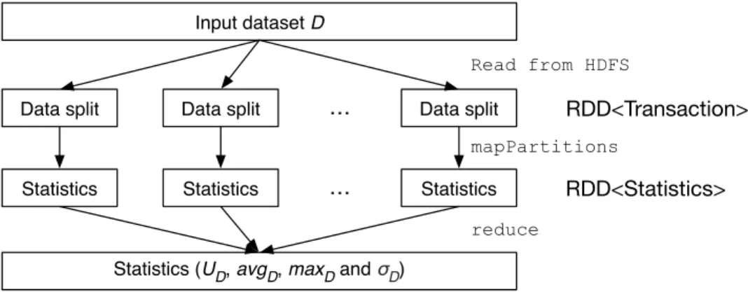
Figure 5.1 illustrates the data flow in Spark for getting the statistics of a dataset. The dataset is first read from HDFS to Spark as a RDD (Resilient Distributed Dataset) of transactions. Then the data in each node is scanned for their statistics. Finally, the statistics are combined. This process is expected to be fast, since only addition and comparison are involved here. In the case that the dataset is so huge that even determining the statistics is not feasible, sampling could also be used here. However, the discussion of this case is out of the scope of this thesis.

It is worth to mention that the way of getting standard deviation of transaction utilities in one pass of database scan is not very obvious. Usually, we use the

(47)

formula σ= v u u t 1 N −1 N X i=1 (xi−x)2 (5.1)

to calculate the standard deviation of xi, i = 1,2, ..., N, where x is the average of

these N values. This formula requires two scans of the values: one is to calculate

x and the other is to calculate the final result. However, (5.1) has an algebraic identity σ = v u u t 1 N −1 " _N X i=1 x2 i ! −N x2 # , (5.2)

which only need one scan of the values.

In order to derive the new theorem later in this section, the following lemmas are discussed first.

Lemma 1. (Hoeffding’s inequality) [24, Theorem 2] IfX1, X2, ..., Xn are

inde-pendent variables, S =X1+X2+...+Xn andai ≤Xi ≤bi(i= 1,2, ..., n), then for

any v >0, P r S n −E S n ≥v ≤exp −2n 2_v2 Pn i=1(bi−ai) 2 ! . (5.3)

Lemma 2. If X1, X2, ..., Xn are independent variables, S =X1+X2+...+Xn and

ai ≤Xi ≤bi(i= 1,2, ..., n), then for any t >0,

P r(|S−E(S)| ≥t)≤2 exp −2t 2 Pn i=1(bi−ai) 2 ! (5.4) Proof. Using a similar proof in [24], we have

P r S n −E S n ≤ −v ≤exp −2n 2_v2 Pn i=1(bi−ai) 2 ! . (5.5)

(48)

From (5.3) and (5.5), P r S n −E S n ≥v ≤2 exp −2n 2_v2 Pn i=1(bi−ai)2 ! . (5.6)

Letv = _nt, so for any t >0,

P r(|S−E(S)| ≥t)≤2 exp −2t 2 Pn i=1(bi−ai) 2 ! . (5.7)

Lemma 3. (Chebyshev’s inequality) Let X (integrable) be a random variable with finite expected value µ and finite non-zero variance σ2. Then for any real number k > 0,

P r(|X−µ| ≥kσ)≤ 1

k2 (5.8)

Lemma 4. Let X1, X2, ..., XN be a set of N independent random variables, and

each Xi has the same probability distribution with mean E(X) and variance σ2.

Then, the average of the N variables X = X1+X2+...+XN

N has a distribution with

mean E(X) = E(X) and variance σ2

X = σ2

N.

Proof. The property of means states that if X and Y are two random variables, then

E(X+Y) = E(X) +E(Y) (5.9) and

(49)

where a and b are constant values.

The property of variances states that ifX andY are two random variables, then

σ_X2₊_Y =σ_X2 +σ_Y2 (5.11) and

σ_a2₊_bX =b2σ_X2, (5.12) where a and b are constant values.

So, E(X) =E X1+X2+...+XN N = E(X1) +E(X2) +...+E(XN) N = N ·E(X) N =E(X) (5.13) and σ_X2 =σ2X1+X2+...+_XN N = σ 2 X1 +σ 2 X2 +...+σ 2 XN N2 = N ·σ2 N2 = σ2 N. (5.14)

In Lemma 4, X1, X2, ..., XN can be a sample drawn from a population. So this

lemma reveals the property of the probability distribution of the sample mean.

5.2 Sampling Strategy

The main challenge in sampling methods is to determine the required sample size to achieve a given accuracy. A new theorem is proposed and proved in this section,

(50)

in order to select the sample size we need.

We derive the following theorem from Lemma 2, 3 and 4:

Theorem 1. Given a dataset D with n transactions, and user given parameters

∈ (0,1), δ ∈ (0,1), k >1. Let S be a random sample of D, so that the size of S,

m ≥ 1 22 maxD avgD 2

ln2_δ, then with probability at least 1−δ− 1

k2, uS(X) US is within the interval h uD(X) UD − +k_√ σD m·avgD ,uD(X) UD + +k_√ σD m·avgD i

, for any itemset X. Proof. Suppose there are m transactions in S: Tg1, Tg2, ..., Tgm. The utilities of

itemsetX in these transactions areu(X, Tg1), u(X, Tg2), ..., u(X, Tgm), which can be

viewed as independent random variables. The values of u(X, Tgi) are bounded:

u(X, Tgi)∈[0, maxD],1≤i≤m. (5.15) Based on Definition 4, uS(X) = u(X, Tg1) +u(X, Tg2) +...+u(X, Tgm). (5.16) According to (5.4) and (5.16), P r(|uS(X)−E[uS(X)]| ≥t)≤2exp − 2t 2 m·maxD2 ,∀t >0. (5.17) Hence, P r uS(X) m −E uS(X) m ≥ t m ≤2exp − 2t 2 m·maxD2 ,∀t >0. (5.18)

(51)

From Lemma 4, E uS(X) m = uD(X) n . (5.19) We have, P r uS(X) m − uD(X) n ≥ t m ≤2exp − 2t 2 m·maxD2 ,∀t >0. (5.20) Hence, P r uS(X) m·avgD − uD(X) n·avgD ≥ t m·avgD ≤2exp − 2t 2 m·maxD2 ,∀t >0. (5.21) Let t=m·avgD, we have

P r uS(X) m·avgD − uD(X) n·avgD ≥ ≤2exp −2m 2_·_avg2 D maxD2 ,∀ >0. (5.22) Since m≥ 1 22 maxD avgD 2

ln2_δ from the pre-condition of the theorem,

2exp −2m 2_·_avg2 D maxD2 ≤δ. (5.23) From (5.22) and (5.23), P r uS(X) m·avgD − uD(X) n·avgD ≥ ≤δ,∀ >0. (5.24) Thus, P r uS(X) m·avgS · avgS avgD − uD(X) n·avgD ≤ ≥1−δ,∀ >0. (5.25) Consequently, P r uS(X) US · avgS avgD − uD(X) UD ≤ ≥1−δ,∀ >0. (5.26)

(52)

From Lemma 4, we also have E(avgS) =avgD (5.27) and σavgS = σD √ m. (5.28)

If σD 6= 0, from Lemma 3 we have

P r |avgS−avgD| ≥k· σD √ m ≤ 1 k2,∀k > 1, (5.29) where avgS is viewed as a random variable.

So, P r avgS avgD −1 ≥k·√ σD m·avgD ≤ 1 k2,∀k > 1. (5.30) Hence, P r avgS avgD −1 ≤k· √ σD m·avgD ≥1− 1 k2,∀k >1. (5.31) In (5.26), if we denote uS(X) US · avgS avgD − uD(X) UD ≤as event A, (5.26) is equivalent toP r(A)≥1−δ. In (5.31), if we denote avgS avgD −1 ≤ k· σD √

m·avgD as event B, (5.31) is equivalent

toP r(B)≥1− 1

k2.

And,

(53)

So, P r(A∧B)≥P r(A) +P r(B)−1≥1−δ− 1 k2, (5.33) which is equivalent to P r uS(X) US · avgS avgD − uD(X) UD ≤∧ avgS avgD −1 ≤k· √ σD m·avgD ≥ 1−δ− 1 k2,∀ >0, k >1. (5.34) Since uS(X) US · avgS avgD − uD(X) UD ≤∧ avgS avgD −1 ≤k·√ σD m·avgD ⇒ uS(X) US − uD(X) UD ≤+ uS(X) US ·k√ σD m·avgD , (5.35) we have P r uS(X) US − uD(X) UD ≤+uS(X) US ·k√ σD m·avgD ≥ P r uS(X) US · avgS avgD − uD(X) UD ≤∧ avgS avgD −1 ≤k·√ σD m·avgD . (5.36) From (5.34) and (5.36), P r uS(X) US − uD(X) UD ≤+uS(X) US ·k√ σD m·avgD ≥ 1−δ− 1 k2,∀ >0, k >1. (5.37)

(54)

And since uS(X) US ≤1, (5.38) consequently, P r uS(X) US − uD(X) UD ≤+k√ σD m·avgD ≥ P r uS(X) US − uD(X) UD ≤+uS(X) US ·k√ σD m·avgD . (5.39) Thus, from (5.37) and (5.39),

P r uS(X) US − uD(X) UD ≤+k√ σD m·avgD ≥1−δ− 1 k2,∀ >0, k >1, (5.40) under the condition that σD 6= 0.

If σD = 0, all the transactions are having the same utility. So avgS = avgD.

From (5.26), P r uS(X) US − uD(X) UD ≤ ≥1−δ,∀ >0. (5.41) So P r uS(X) US − uD(X) UD ≤+k√ σD m·avgD ≥ P r uS(X) US − uD(X) UD ≤ ≥1−δ≥1−δ− 1 k2,∀ >0, k >1, (5.42) under the condition that σD = 0.

To sum up, P r uS(X) US − uD(X) UD ≤+k√ σD m·avgD ≥1−δ− 1 k2,∀ >0, k >1, (5.43)

(55)

under all conditions, which concludes that for any itemsetX, ifm≥ 1 22 maxD avgD 2 ln2_δ, then with probability at least 1−δ− 1

k2, uS(X)

US is within the interval

h_u D(X) UD − +k_√ σD m·avgD ,uD(X) UD + +k_√ σD m·avgD i .

For simplicity, we denote

ω(, δ, D) = 1 22 maxD avgD 2 ln2 δ (5.44) and 0 =+k√ σD m·avgD (5.45)

in the rest of this thesis.

In the final results, if the minimum threshold is θ, we output all the itemsets with utility at least (θ−0)US in sample S of size at least ω(, δ, D).

It is worth to mention that ω(, δ, D) is independent of the size of the original dataset. The only factor from the dataset comes from the statistics of it, i.e. maxD

and avgD. When the dataset becomes larger, if max_avgD

D does not change much, the

required sample size will also stays similar. In general, we can expect that avgD

does not change much, and maxD grows slowly as the dataset size becomes bigger.

If some transactions makemaxD much higher than the majority of the transactions,

we can also remove these transactions, since they are usually considered outliers. We hereby prove that the accuracy of our results is guaranteed.

(56)

Theorem 2. With minimum threshold θ, if we output all the itemsets with utility at least (θ−0)US in sample S of size at least ω(, δ, D), itemset X is output with

probability at least 1−δ− 1

k2, if X is an HUI in dataset D.

Proof. Since itemsetX is an HUI, according to the definition of HUI, we have

uD(X)≥θUD. (5.46) Hence, uD(X) UD −0 ≥θ−0. (5.47) According to Theorem 1, uS(X) US ≥ uD(X) UD −0 (5.48)

with probability at least 1−δ− 1

k2.

From 5.47 and 5.48, we have

uS(X)

US

≥θ−0 (5.49)

k2.

So X is output with probability at least 1−δ− 1

k2.

Theorem 3. With minimum threshold θ, if we output all the itemsets with utility at least (θ−0)US in sample S of sample size at least ω(, δ, D), any itemsets in

the output are guaranteed to have a utility at least (θ−20)UD in dataset D with

probability at least 1−δ− 1

(57)

Proof. Suppose itemsetX is output, we have uS(X)≥(θ−0)US. (5.50) Hence, uS(X) US ≥θ−0. (5.51) According to Theorem 1, uS(X) US ≤ uD(X) UD +0 (5.52)

k2.

From 5.51 and 5.52, we have

θ−0 ≤ uD(X)

UD

+0 (5.53)

k2.

Hence,

uD(X)

UD

≥θ−20 (5.54)

k2.

So X has a utility at least (θ −20)UD in dataset D with probability at least

1−δ− 1

k2.

There are 3 parameters used in this sampling strategy, namely , δ and k. The value of k determines a base value for the probability bound. k will be set to 2

(58)

in our experiments. The reason for choosing this value for k will be explained in Section 6.2. The value ofδ, in the range of (0,1), determines the probability bound together with k. If users want to have more confidence in the results, δ could be set to a lower value, and the required sample size will be bigger. , in the range of (0,1), is the extra error bound for the relative utility, i.e. error in addition to

k_√ σD

m·avgD. Choosing a smaller value for will lead to more accurate results, but a

bigger required sample size. So choosing the values forδ and is very important in the sampling strategy. We need to make sure that the values for parameters will not result in a sample size even bigger than the total size of the dataset. Also, we want the error bound to be low and the probability bound to be high, so that the results could have a relatively high accuracy and confidence. In my experiments, we usually choose the value of to be ₁₀1 of the relative utility threshold. If the required sample size is too big compared to the total size of the dataset, the value of will be increased a little bit for looser error bound and smaller sample size.

5.3 PHUI-Miner with Sampling

The sampling method mines an approximate set of HUIs, but reduces the size of the dataset to ω(, δ, D) as shown in this chapter. However, in most cases, a sample with size ω(, δ, D) is still too large to mine for a single machine. Besides, the parallel distributed algorithm proposed in the previous chapter also has the

(59)

running time issue, when the dataset gets bigger. Our solution to this problem is to combine the two methods, so that the dataset is sampled before being processed byPHUI-Miner.

In this section, an approach combining sampling and PHUI-Miner, referred to as,PHUI-Miner with Sampling, is proposed.

Given a dataset D, a minimum relative utility threshold θ, user provided pa-rameters δ, and k. Theorem 1 guarantees that if we only use a sample of Dwith size ω(, δ, D), and mine all the itemsets with relative utility no less than θ −0, any high utility itemsetX will appear in the output with probability 1−δ− 1

k2.

Our approach first draws a sample with size ω(, δ, D) from the whole dataset, and then mines HUIs with threshold θ −0 parallelly with PHUI-Miner. In this way, PHUI-Miner with Sampling is able to achieve the same accuracy as using a single machine to mine a sample of the dataset, and have better time and memory performance than usingPHUI-Miner alone.

(60)

6 Experimental Results

The parallel distributed algorithm PHUI-Miner and the sampling method, pro-posed in this thesis, are evaluated in this chapter. The evaluations are focused on the time performance of PHUI-Miner, and the accuracy of the sampling method. Experiments are also conducted to evaluate the time performance of PHUI-Miner with Sampling in Section 6.1.

In our experiments, parallel distributed algorithms are run on Amazon Web Services (AWS). We used twenty r3.xlarge instances to run HDFS and Spark on them. One of the instances is used as Master, while the others are Workers. The non-parallel algorithms are conducted on a single Intel(R) Xeon(R) X5660 computer with 50 GB of RAM.

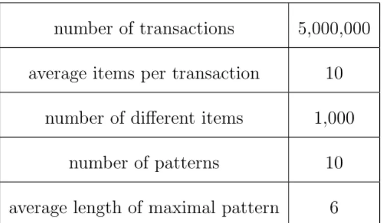
The experiments are conducted on different datasets,kosarak[19],accidents[19], chess[19],twitter[26],T5000L10I1P10PL6,ta-feng[4] andglobe. T5000L10I1P10PL6 is a synthetic dataset, while the other six are real-world datasets. T5000L10I1P10PL6 is generated using the IBM Quest Data Generator [21]. The IBM Quest Data

(61)

number of transactions 5,000,000 average items per transaction 10

number of different items 1,000 number of patterns 10 average length of maximal pattern 6

Table 6.1: Parameters of the Synthetic Dataset

Generator is often used in studies of frequent pattern mining and association rule mining, and can generate datasets without utilities according to input parameters. The parameters for the synthetic dataset used in this paper are shown in Table 6.1. For T5000L10I1P10PL6, the internal utilities are generated using a uniform distribution in [1,10], while the external utilities are generated using a log-normal distribution, with µ = 1 and σ = 0.5. The kosarak dataset contains anonymized click-stream data of a Hungarian online news portal, which is a sparse dataset. The accidents dataset consists of a collection of traffic accident records. Each record contains a description of an accident such as gender of the driver, speed limit of the road, and whether alcohol is involved. The chess dataset is derived from chess game steps, which is very dense. The utility values for kosarak, acci-dentsand chess are taken from [19], where the internal utility values are generated using a uniform distribution in [1,10] and the external utility values are generated

(62)

using a normal distribution. The twitter dataset describes the followers of Twitter users, in which each transaction corresponds to a user and contains the list of fol-lowers of the user. For thetwitter dataset, the internal utilities are generated using a log-normal distribution, with µ = 2.22 and σ = 0.6. The external utilities are generated using a log-normal distribution, with µ = 0 and σ = 0.1. The ta-feng dataset is from a supermarket in Taiwan and describes the transactions collected within a time span of four months, from November, 2000 to February, 2001. There are a total of 119,578 transactions involving 24,069 products and 32,266 customers in the dataset [33], which contains profits of each merchandise. The globe dataset comes from The Globe and Mail [5], which is a news company in Canada. Each transaction in theglobe dataset represents page views of a visitor in one time. The items are the titles of articles, while the internal utilities are the times spent on the articles and the external utilities are all 1’s. The reason for choosing the values in T5000L10I1P10PL6andtwitteris that, in the sampling method, the resulting sam-ple sizeω(, φ, D) should be smaller than the original dataset. Otherwise, we should mine the HUIs using the original dataset without sampling. We also trimmed the lengths of transactions in twitterto at most 15 for simplicity.

Below, we first present the performance of PHUI-Miner and PHUI-Miner with Sampling. Then, the accuracy of the sampling strategy will be evaluated. Finally, the application of high utility itemset mining will be discussed.

(63)

6.1 PHUI-Miner and PHUI-Miner with Sampling

SincePHUI-Mineris an exact approach, there is no need for the accuracy evaluation for it. The evaluation of PHUI-Miner is conducted in terms of time performance and speedup. We also evaluate the time performance ofPHUI-Miner with Sampling in this section.

To better evaluate our algorithm, we designed an algorithm, calledPHUI-Miner Rnd, for comparison purpose. The PHUI-Miner Rnd algorithm is the same as PHUI-Miner except for the Split Search Space phase. In PHUI-Miner Rnd, the items are split randomly into different nodes instead of using the procedure shown in Algorithm 3. Comparing PHUI-Miner Rnd with PHUI-Miner shows that the choice of the way of splitting the search space in our designing of PHUI-Miner is reasonable. Experiments on PHUI-Miner Rnd are conducted at least 5 times for each experiment to get average results.

Below, the time performance of PHUI-Miner and PHUI-Miner with Sampling is first presented. And then, the speedup of PHUI-Miner is evaluated.

6.1.1 Time Performance

To the best of our knowledge, very few studies have been proposed to use distributed computing technique to mine high utility itemsets. Thus, the time performance of

(64)

PHUI-Miner is evaluated against HUI-Miner and PHUI-Miner Rnd, while PHUI-Miner with Samplingis compared with PHUI-Miner.

Since the datasets twitter and T5000L10I1P10PL6 consume too much mem-ory as well as running time, HUI-Miner is not able to mine these two datasets. So the comparison of PHUI-Miner and HUI-Miner is only conducted on kosarak, accidents, chess, ta-feng and globe. Figures 6.1a, 6.1b, 6.1c, 6.1f and 6.1g show the results for comparing PHUI-Miner with HUI-Miner. Our method outperforms HUI-Miner in all the cases. However, when the relative utility threshold is big, the time performance of HUI-Miner approaches PHUI-Miner. This is because of the network latency the cluster introduces. PHUI-Miner will need at least some time to read the data from the HDFS, repartion the data, etc. When the threshold is small, and a large amount time is needed in the mining process. PHUI-Miner works much better than HUI-Miner.

Figure 6.1 also shows the time performance of PHUI-Miner and PHUI-Miner Rnd. In kosarak, accidents, chess, ta-feng and globe, the time performances of the two methods are similar. However, PHUI-Miner is slightly faster than PHUI-Miner Rnd in these datasets. For the twitter dataset, PHUI-Miner works much better than PHUI-Miner Rnd. For the T5000L10I1P10PL6 dataset, PHUI-Miner is slightly slower than PHUI-Miner Rnd though. These are normal behaviours, since the distributions of different datasets are different. Some datasets may have

(65)

very special distribution, that our approach is not the optimal solution to them. However, it is shown that in most cases, PHUI-Miner works better than PHUI-Miner Rnd. In the cases that PHUI-Miner works slower, the difference of them is very small. As a result, our way of splitting the search space is demonstrated to be a good choice.

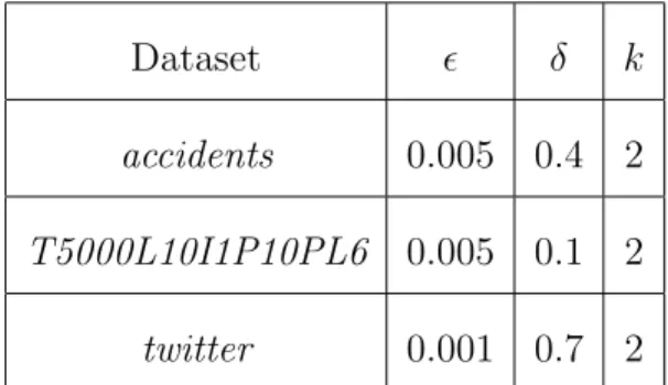
For the comparison of PHUI-Miner withPHUI-Miner with Sampling, it is only conducted on datasets accidents, twitter and T5000L10I1P10PL6. The other four datasets are not suitable for the sample technique, since their minimum required sample sizes exceed the sizes of the whole datasets. Figures 6.1b, 6.1d and 6.1e show the experimental results of the time performance for PHUI-Miner with Sam-pling and PHUI-Miner. The values of other parameters used in PHUI-Miner with Sampling in this section are provided in Table 6.2. It’s demonstrated that PHUI-Miner with Samplinghas better time performances in all three datasets. In datasets twitter and T5000L10I1P10PL6, which have millions of transactions, PHUI-Miner with Sampling is much faster than PHUI-Miner.

6.1.2 Speedup

The speedup forPHUI-Mineris evaluated on thekosarakdataset. We used different number of nodes to run the experiments, regarding the speed using two nodes as 1. The results are in Figure 6.2. The relative utility threshold used for kosarak

(66)

(a) 8 9 10 11 x 10−3 0 0.5 1 1.5 2 2.5 3x 10 5

Relative Utility Threshold

running time (ms) PHUI−Miner PHUI−Miner Rnd HUI−Miner (b) 0.080 0.1 0.12 0.14 0.16 0.18 0.5 1 1.5 2 2.5x 10 6

running time (ms)

PHUI−Miner PHUI−Miner Rnd HUI−Miner

PHUI−Miner with Sampling

(c) 0.17 0.18 0.19 0.2 0.21 0 2 4 6 8 10x 10 5

running time (ms)

(67)

(d) 3.9 4 4.1 4.2 4.3 4.4 4.5 4.6 4.7 x 10−3 0.8 1 1.2 1.4 1.6 1.8 2x 10 5

running time (ms)

PHUI−Miner PHUI−Miner Rnd PHUI−Miner with Sampling

(e) 0.028 0.03 0.032 0.034 0.036 0.038 0.04 0.042 0.044 1 2 3 4 5x 10 5

running time (ms)

PHUI−Miner PHUI−Miner Rnd PHUI−Miner with Sampling

(f) 4.8 5 5.2 5.4 5.6 5.8 6 x 10−4 3 3.5 4 4.5 5 5.5x 10 4

running time (ms)

(68)

Dataset δ k

accidents 0.005 0.4 2 T5000L10I1P10PL6 0.005 0.1 2 twitter 0.001 0.7 2

Table 6.2: Values of Parameters

(g) 2 2.5 3 3.5 4 4.5 5 5.5 x 10−5 2 4 6 8 10 12x 10 4

running time (ms)

Figure 6.1: Running Time of PHUI-Miner on (a) kosarak, (b) accidents, (c) chess, (d) twitter, (e) T5000L10I1P10PL6, (f) ta-feng and (g)globe

(69)

2 5 8 11 14 17 20 1 1.1 1.2 1.3 1.4 1.5 # of machines Speedup

Figure 6.2: Speedup of PHUI-Miner

is 0.01. It’s shown that the speedup of PHUI-Miner is near linear, which means our approach could scale well when we have more and more nodes. However, it is notable that our algorithm could not have a linear speedup when we have a large number of nodes. If there are too many nodes, the communication cost will be dominating the total running time. But if the number of nodes is not very big, the computation cost is the main cost.

6.2 Accuracy of Sampling Strategy

In order to evaluate the accuracy of our sampling strategy, we have performed several experiments on accidents, T5000L10I1P10PL6 and twitter.

The statistics for the three datasets are in Table 6.3.

(70)

Dataset twitter T5000L10I1P10PL6 accidents # of transactions 19,265,416 4,947,263 340,183

maximum utility 456 788 1034

average utility 121.15 196.04 576.58

Table 6.3: Statistics of Datasets in the Sampling Strategy

Dataset θ k

accidents 0.085 0.005 2 T5000L10I1P10PL6 0.03 0.005 2 twitter 0.004 0.001 2

Table 6.4: Values of Parameters

on mining samples drawn from different datasets. We evaluate the effectiveness of the proposed sampling method against the exact results and provide the precision, recall, f-measure and relative utility error of our method on the three datasets. The relative utility error is computed as the utility error compared with the exact utility results:

relative utility error =

approximate utility−exact utility exact utility . (6.1) Since ω(, δ, D) is independent of the total size of the dataset, even when the dataset is very small, it’s still possible that a huge dataset size is required for a

(71)

(a) 0 0.2 0.4 0.6 0.8 0 1 2 3 x 105 δ Sample size total size: 340,183 (b) 0 0.2 0.4 0.6 0.8 0 1 2 3 4 5 x 106 δ Sample size total size: 4,947,263 (c) 0.2 0.3 0.4 0.5 0.6 0.7 0 0.5 1 1.5 2 x 107 δ Sample size total size: 19,265,416

(72)

0.5 0.7 0.9 1.1 1.3 1.5 1.7 1.9 x 107 5 6 7 8 9 10 11x 10 5 Size of dataset Sample size

Figure 6.4: Sample Sizes for Different Sizes of Datasets

given accuracy according to our theorem, depending on the data distribution of the dataset, while for some datasets, only a small fraction of the whole dataset is required. Figure 6.3 presents the required sample size of the three datasets for different δ’s. The values for other parameters used in this section are shown in Table 6.4. The sample sizes grow exponentially as δ decreases. However, if a reasonable δ is chosen, the sample size is usually much smaller than real-world big datasets, that can have billions of transactions. Figure 6.4 shows the sample size for different sizes of datasets. The datasets used in this figure are all generated using the IBM Quest Data Generator with the same parameters as used in generating T5000L10I1P10PL6except the dataset size. The sample size in this figure is shown to be not very related to the total size of the dataset. The sample size gets slightly

(73)

bigger as the total size gets bigger because the value of maxD is more likely to get

bigger.

It is worth to mention that we chose the values for’s in Table 6.4 according to the characteristics of the datasets. ’s are chosen so thatis much smaller thanθso as to have a good accuracy. In the meanwhile,’s cannot be too small, since smaller

values result in bigger sample sizes. We chose 2 fork’s in all the datasets, since the probability 1−δ− 1

k2 would be 0.75−δ, which is acceptable in our experiments. If

k is bigger, the threshold θ−0 used for mining would be smaller, which will affect the accuracy and running performance of the sampling strategy. If k is smaller, the probability guarantee of 1−δ− 1

k2 would be smaller. For the same reason, we

choose the same value for k’s in Section 6.1.

In our experiments, in order to better measure the accuracy of our algorithms, we used a measure called precision with AFPs. Since our approach is to find all HUIs with relative utility at leastθ−0, the HUIs with relative utility in the range of [θ−0, θ), calledAcceptable False Positives(AFPs), are considered as true positives in our results when computing the precision with AFPs. Correspondingly, we use f-measure with AFPs to replace the commonly used f-measure.

Figure 6.5 shows the precision with AFPs, recall, and f-measure with AFPs for different δ values. The recall is constantly 1, which means all the exact high utility itemsets are found, although our theorem only guarantees that a high utility

(74)

(a) 0 0.2 0.4 0.6 0.8 0.9 0.92 0.94 0.96 0.98 1 δ Accuracy

precision with AFPs recall

f−measure with AFPs

(b) 0 0.2 0.4 0.6 0.8 0.9 0.92 0.94 0.96 0.98 1 δ Accuracy

(c) 0.2 0.3 0.4 0.5 0.6 0.7 0.9 0.92 0.94 0.96 0.98 1 δ Accuracy

Figure 6.5: Accuracy of Sampling on (a) accidents, (b) T5000L10I1P10PL6 and (c) twitter

(75)

(a) 0 0.2 0.4 0.6 0.8 0.2 0.4 0.6 0.8 1 δ Accuracy precision recall f−measure (b) 0 0.2 0.4 0.6 0.8 0.2 0.4 0.6 0.8 1 δ Accuracy precision recall f−measure (c) 0.2 0.3 0.4 0.5 0.6 0.7 0 0.2 0.4 0.6 0.8 1 δ Accuracy precision recall f−measure

Figure 6.6: Accuracy of Sampling without AFPs on (a) accidents, (b) T5000L10I1P10PL6and (c) twitter

(76)

(a) 0 0.2 0.4 0.6 0.8 0 0.005 0.01 0.015 0.02 0.025 0.03 δ

Relative utility error

(b) 0 0.2 0.4 0.6 0.8 0 0.005 0.01 0.015 0.02 0.025 0.03 δ

(c) 0.2 0.3 0.4 0.5 0.6 0.7 0 0.005 0.01 0.015 0.02 0.025 0.03 δ

Figure 6.7: Average Value and Standard Deviation of Relative Utility Error on (a) accidents, (b) T5000L10I1P10PL6 and (c)twitter