Radu Baltean-Lugojan† and Panos Parpas†
Abstract. Implied volatility expansions allow calibration of sophisticated volatility models. They provide an accurate fit and parametrization of implied volatility surfaces that is consistent with empirical ob-servations. Fine-grained higher order expansions offer a better fit but pose the challenge of finding a robust, stable and computationally tractable calibration procedure due to a large number of market parameters and nonlinearities. We propose calibration schemes for second order expansions that take advantage of the model’s structure via exact parameter reductions and recoveries, reuse and scaling between expansion orders where permitted by the model asymptotic regime and numerical iteration over bounded significant parameters. We perform a numerical analysis over 12 years of real S&P 500 index options data for both multiscale stochastic and general local-stochastic volatility models. Our methods are validated empirically by obtaining stable market parameters that meet the qualitative and numerical constraints imposed by their functional forms and model asymptotic assumptions. Key words. implied volatility expansions, numerical calibration, parameter reductions, nonlinear least squares AMS subject classifications. 91G20, 91G60, 90C30, 60-08
1. Introduction. Research into implied volatility modelling both in academia and indus-try is focused on addressing the unrealistic assumption of constant asset volatility in the well-known Black-Scholes framework for pricing financial options (see [13] for an overview). A robust model parametrization of implied volatility needs to capture both characteristics and dynamics of the implied volatility surface along different strikes and maturities (or ex-piries). In addition, volatility models need to balance parameter stability with quality of fit over market data. Practitioners often prioritize tight fits and re-calibrate daily due to overfits that are not stable over multiple days. Meanwhile, existing literature focuses more on consis-tency. The downside of models that focus on consistency is that they can be computationally expensive to calibrate or are narrowly applicable in pricing a range of derivative contracts. The literature around volatility models is substantial, and we refer the reader to [10] for an extensive overview and comparison of volatility model classes.
Models that consistently capture detailed volatility dynamics typically require calibration via numerical-based approaches that are often computationally expensive or lead to numerical instabilities. In order to address these issues, theoretical results have been proposed that translate model formulations into explicit implied volatility expansions for an alternative faster parameter calibration. Fouque et al [8, 9] studied Stochastic Volatility (SV) models with multiple factors driving volatility on different time scales. These multifactor models have been validated by empirical studies that show that the deterministic volatility assumption is inconsistent with real data [2]. Instead, studies find that volatility is strongly mean-reverting [15] and show the presence of multiple time scales (or dimensions) of volatility variation [7,16]. More recently, Lorig et al [14] adopted a general class of multifactor Local-Stochastic Volatility (LSV) models with hybrid dynamics. For an extensive review of local-stochastic
†
Department of Computing, Imperial College London, 180 Queen’s Gate, London, SW7 2AZ, UK ([email protected], [email protected]).
modelling see [12]. Both multiscale SV and LSV models are based on explicit asymptotic approximations of implied volatility in successive orders of perturbation [9] and Taylor [14] expansions, respectively.
The implied volatility Second Order Expansions (SOE) for both SV and LSV model classes considered are explicit nonlinear functions of market parameters. Each successive order of expansion leads to an explosion in the number of market parameters (in SOE - 18 for SV, 13 for LSV). Therefore, calibrating to European options market data requires a two-step procedure. First, a coefficient set is easily obtained by regressing around multiple basis functions of forward log-moneyness and maturity. The main difficulty lies in the second step of translating coefficients into a minimal l2-norm set of required market parameters. Finding SOE market
parameters from coefficients for both model expansions considered involves a complex least-norm minimization problem with nonlinear polynomial constraints exhibiting non-convexity, with no guarantee of a globally optimal solution and a computationally intractable search of the parameter space even when using state of the art global solvers. Furthermore, non-robust solutions can introduce large parameter instability over time, whereas the stability of market parameters is crucial for minimizing hedging costs when using them as a volatility surface parametrization for pricing exotics [5,6].
Motivated by the above, the focus of this paper is to propose tractable, data-validated calibration schemes to obtain stable market parameters from coefficients in second order im-plied volatility expansions (SOE). We illustrate our methods and numerical analysis for both the SV and LSV model classes cited above. Our methods consist of parameter reduction and recovery (via grouping or gradients), reuse of lower order expansions where the order mag-nitude separation allows it and numerical iteration over bounded and interpretable market parameters. We also perform a detailed numerical analysis on 12 years of S&P 500 European options data (2000-2011) showing a tight fit and stable set of SOE market parameters for both of the SV and LSV calibration schemes we propose.
The rest of the paper proceeds as follows: in section 2we review the model formulations, implied volatility expansion results up to SOE and their implications for both (multiscale) SV and LSV models; insection 3we construct our proposed calibration schemes; in section 4we illustrate SOE calibration on index options data in terms of fit and stability for both models and we compare the results; in section 5 we discuss our results, implications and possible extensions.
2. Models Considered. We introduce two classes of implied volatility models. Both model classes provide successive option price expansions which are translated into successive approxi-mating calibration formulas to the implied volatility surface. We present the theoretical results from [9] and [14] needed in each model class for practical calibration of market parameters within a second order expansion and discuss the calibration challenges of existing approaches and motivate our proposed solution.
2.1. Multiscale SV with Perturbation Expansions. Fouque et al [8, 9] develop implied volatility expansions for a class of two-factor two-scale volatility models defined under the
risk-neutral pricing measureP by the system of stochastic differential equations: (1) dXt=rXtdt+f(Yt, Zt)XtdWt(0), dYt= 1 α(Yt)− 1 √ β(Yt)Λ1(Yt, Zt) dt+√1 β(Yt)dW (1) t , dZt= δc(Zt)− √ δg(Zt)Λ2(Yt, Zt) dt+ √ δg(Zt)dWt(2),
where (Wt(0), Wt(1), Wt(2)) are correlated Brownian motions, r is the risk-free rate and Yt,
Zt describe fast and slow volatility factors/scales characterized by fixed scaling parameters 0< , δ 1. The assumed small-, small-δ regime leads to a second order expansion (SOE) in powers of the scales √,√δ, providing the following approximation to implied volatility:
(2) I ≈I0,0+ √ I1,0+ √ δI0,1+ √ δI1,1+I2,0+δI0,2+... :=ISV(τ, d; Θ) = 1 τk+l+τ m+τ 2n +d τ p+τ q+τ 2s + d 2 τ2 u+τ v+τ 2w +O(1+q/2+√δ+δ√+δ3/2), ∀q <1,
whereτ, d represent time-to-maturity and forward log-moneyness respectively, and Θ :={k, l, m, n, p, q, s, u, v, w},
is theestimated coefficient set. The set Θ is obtained via a nonlinear mapping f :R18→R10 on a set Φ of market parameters that are required for pricing and hedging exotics and represent functional forms of the model coefficient functionsα, β, c, g,Λ1,Λ2. In particular, we have
(3) Θ =f(Φ), Φ : ={σ∗, V3, V1δ, V0δ, C2,δ, C1,δ, C0,δ, C,δ, A2, A1, A0, A, B2δ, B1δ,V 0 3 σ0 , V10δ σ0 , V00δ σ0 , φ },
where the mapping f represents the following system of nonlinear equations: (4a) O(1 τ) : k= 3(V3)2 2(σ∗)5 − A2 (σ∗)3 − A (σ∗)3 − φ 2σ∗, O(1) : l= 3V δ 1V3 (σ∗)4 − C2,δ 2(σ∗)2 − C,δ 2(σ∗)2 + A0 σ∗ + A1 2σ∗ + A2 4σ∗ − A 4σ∗ − V1δV30 (σ∗)3σ∗0 +σ ∗+ V3 2σ∗, O(τ) : m= B δ 1 2 + C0,δ 2 + C1,δ 4 + C2,δ 8 − C,δ 8 + 5(V1δ)2 6(σ∗)3 − V0δV3 2(σ∗)2 + B2δ 6σ∗ − 2V δ 1V10δ 3(σ∗)2σ∗0 + Vδ 0V30 2σ∗σ∗0 + Vδ 1V30 4σ∗σ∗0 +V δ 0 + Vδ 1 2 , O(τ2) : n= (V δ 0)2 6σ∗ + V0δV1δ 6σ∗ + (V1δ)2 6σ∗ − B2δσ∗ 12 + 2V0δV00δ 3σ∗0 + V00δV1δ 3σ∗0 + V0δV10δ 3σ∗0 + V1δV10δ 6σ∗0 , O(d r) : p=− 3(V3)2 2(σ∗)5 + A1 (σ∗)3 + A2 (σ∗)3 + V3 (σ∗)3,
(4b) O(d) : q =−3V δ 0V3 (σ∗)4 − 3V1δV3 (σ∗)4 + C1,δ 2(σ∗)2 + C2,δ 2(σ∗)2 + V0δV30 (σ∗)3σ∗0 + V1δV30 (σ∗)3σ∗0 + V1δ (σ∗)2, O(dτ) : s=−5V δ 0V1δ 3(σ∗)3 − 5(V1δ)2 6(σ∗)3 + 2V00δV1δ 3(σ∗)2σ∗0 + 2V0δV10δ 3(σ∗)2σ∗0 + 2V1δV10δ 3(σ∗)2σ∗0, O(d 2 τ2) : u=− 3(V3)2 (σ∗)7 + A2 (σ∗)5 + A (σ∗)5, O(d 2 τ ) : v=− 6V1δV3 (σ∗)6 + C2,δ 2(σ∗)4 + C,δ 2(σ∗)4 + V1δV30 (σ∗)5σ∗0, O(d2) : w=−7(V δ 1)2 3(σ∗)5 + B2δ 3(σ∗)3 + 2V1δV10δ 3(σ∗)4σ∗0.
In [9], the authors propose the following two-step calibration procedure:
1. Find Θ∗ that minimizes the least-squares fit error over all maturities iand strikesj:
(5) Θ∗= arg min Θ X i X j I(τi, dj)−ISV(τi, dj; Θ) 2 . 2. Find Φ∗ by solving the following constrained optimization problem:
(6) Φ∗ = arg min
Φ∈J
kΦk2, given J ={Φ : Θ∗ =f(Φ), f :=(4)}.
The first order expansion (FOE) presented in [8] has the reduced form
(7) I ≈I0,0+ √ I1,0+ √ δI0,1 = (l1+τ m1) + d τ (p1+τ q1), l1 =σ?+ V3 2σ?, m1=V δ 0 + V1δ 2 , p1 = V3 σ?3, q1 = V1δ σ?2,
and retains only parameters σ?, V0δ, V1δ, V3 which can be directly obtained from l1, m1, p1, q1
after fitting them to the implied volatility data maturity-by-maturity.
The superscripts of all market parameters in Φ(3) except forσ∗, where present, indicate dependence on volatility factor scales , δ. In [8,9] the authors show , δ dependence can be factored out explicitly:
(8) O( √ ) : Vi =√Vi, Vi0(z) :=∂zVi(z); O( √ δ) : Viδ = √ δVi, Vi0δ(z) :=∂zViδ(z); O() : Ai =Ai, φ(y, z) :=φ(y, z); O(δ) : Biδ :=δBi; O( √ δ) : Ci,δ := √ δCi.
Remark 1. The√,√δ power orders for the terms appearing both in SOE coefficientsΘin (4)and in FOE coefficients{l1, m1, p1, q1}act as a direct link to the implied volatility expansion (2). Due to the small-, small-δ model regime the , δ scaling variables also induce orders of magnitude through their √,√δ power orders. The terms appearing in FOE coefficients
{l1, m1, p1, q1} are zero or first order (O(1),O(
√
),O(√δ)), while the terms in {k, l−l1, m−
m1, n, p−p1, q−q1, s, u, v, w} are of second order (O(), O(δ), O(
√
δ)) and act as a second order magnitude correction to the first order volatility approximation (7).
2.2. LSV with Taylor Expansions. Lorig et al [14] derive implied volatility expressions based on time-independent Taylor expansions within the more general framework of Local-Stochastic Volatility (LSV) models of the type (one volatility factor case),
(9) dXt= r(t)−σ0(t, Xt, Yt) 2 2 dt+σ0(t, Xt, Yt)dWt(0), X0 =x∈R, S=eX, dYt=µ1(t, Xt, Yt)dt+σ1(t, Xt, Yt)dWt(1), Y0=y ∈R, dhW0, W1it=ρ(t, Xt, Yt)dt, |ρ|<1,
where we introduced a deterministic interest rate r(t) to be consistent with the previous SV model class. For the second order expansion (SOE), the authors in [14] obtain the implied volatility approximation,
(10) I ≈I0+I1+I2:=ILSV(τ, d; Θ) =l+τ m+τ2n+dq+d2w+τ ds,
where τ, d represent time-to-maturity and forward log-moneyness (due to introducing non-zero rates) respectively and,
Θ :={l, m, n, q, w, s},
is the estimated coefficient set. Again Θ is dependent on the set Φ of market parameters via a nonlinear mapping g:R13→R6. In particular, we have
(11) Θ =g(Φ), Φ :={a0,0, a0,1, a1,0, a1,1, a0,2, a2,0, b0,0, c0,0, c0,1, c1,0, f0,0, f0,1, f1,0}, (12) a:= σ 2 0 2 , b:= σ21 2 , c:=ρσ0σ1, f :=µ1, ∀η ∈ {a, b, c, f} ηi,j = ∂ix∂yjη(x, y) i!j! , where the mapping g represents the following system of nonlinear equations:
(13a) O(1) :l=p2a0,0=σ0, O(τ) :m= a0,1(c0,0+ 2f0,0) 4σ0 + a2,0σ0 12 − a21,0 8σ0 +a1,1c0,0 12σ0 +a0,1a1,0c0,0 12σ03 − a0,1c1,0 6σ0 +a0,2b0,0 2σ0 −a0,2c 2 0,0 6σ3 0 +3a 2 0,1c20,0 8σ5 0 −a 2 0,1b0,0 3σ3 0 −a0,1c0,0c0,1 6σ3 0 , O(τ2) :n= −a 2 1,0σ0 96 − a0,1a1,0c0,0 48σ0 −a 2 0,1b0,0 12σ0 +a0,1c0,0c0,1 24σ0 +a0,1c0,0f0,1 12σ0 −a 2 0,1c0,0f0,0 8σ03 +a0,1c0,1f0,0 12σ0 + a0,1f0,0f0,1 6σ0 −a 2 0,1f02,0 8σ03 + a0,2(c0,0+ 2f0,0)2 24σ0 , O(d) :q = a1,0 2σ0 +a0,1c0,0 2σ03 , O(d2) :w= a2,0 6σ0 −a 2 1,0 4σ3 0 + a1,1c0,0 6σ3 0 −5a0,1a1,0c0,0 6σ5 0 +a0,1c1,0 6σ3 0 +a0,2c 2 0,0 6σ05 − 3a20,1c20,0 4σ07 + a20,1b0,0 3σ50 + a0,1c0,0c0,1 6σ05 ,
(13b) O(τ d) : s= a1,1(c0,0+ 2f0,0) 12σ0 +a0,1(c1,0+ 2f1,0) 12σ0 −5a1,0a0,1(c0,0+ 2f0,0) 24σ3 0 +a0,1c0,1f0,0 6σ3 0 +c0,0a0,1(c0,1+ 2f0,1) 6σ03 − 3a20,1c0,0(c0,0+ 2f0,0) 8σ05 + a0,2c0,0(c0,0+ 2f0,0) 6σ30 .
A similar two-stage calibration problem to the one described in subsection 2.1is used: 1. Find Θ∗ such that,
(14) Θ∗ = arg min Θ X i X j I(τi, dj)−ILSV(τi, dj; Θ) 2 .
2. Find Φ∗ such that,
(15) Φ∗ = arg min
Φ∈J
kΦk2, given J ={Φ : Θ∗ =g(Φ), g:=(13)}. A Taylor first order expansion (FOE) approximation takes the form,
(16) I ≈I0+I1 =l+τ m1+dq, m1 =
a0,1(c0,0+ 2f0,0)
4σ0
.
Remark 2. All parameters a0,1, a1,1, c0,0, c1,0, f0,0, f1,0 can have signs inverted at the same time in problem (15) with no impact on Φ∗ and without violating the constraints in (13). Therefore we are required to make a choice constraining the sign of one parameter to pick one of two alternative solutions with identical optimal value Φ∗. We choose f0,0, representing the drift rate of the additional process, to be negative, a choice consistent with the negative f0,0 obtained when specializing (9) to SABR model [11] dynamics in [14].
The choice of negativef0,0 does not preclude obtaining results consistent with other special-ized LSV models having the same explicit time-independent Taylor expansions. For instance, to be consistent with the 3/2 model expansion in [14], parameter a0,1 must be positive, which again imposes a sign choice. We can easily convert numerical results obtained by following SABR assumptions to be consistent with 3/2 assumptions by enforcing a0,1 to be positive instead i.e. flipping signs of parameters a0,1, a1,1, c0,0, c1,0, f0,0, f1,0 if a0,1 is negative.
Remark 3. Unlike the SV model (see Remark 1), the LSV implied volatility expansion is built with no explicit scaling and therefore no order of magnitude separation between successive expansions. This precludes the reuse of FOE results (16) as part of the calibration procedure of the SOE.
2.3. Calibration Issues. To compute the coefficient set Θ∗ for both SV and LSV second order expansions, the observed volatility surface is fitted across all maturities at once. The coefficients resulting in a least squares fit globally across the volatility surface can be found using a local solver (for example Matlab’s ‘fmincon’) because the fit is linear in all coefficients. However, the second step of finding the market parameters set Φ∗ from Θ∗ via either
highly non-trivial due to the nonlinear systems of equations (4) and (13) linking Φ∗ to Θ∗ in the case of the SV and LSV models, respectively. More specifically, the inversion steps
(6) and (15) require solving a global non-convex constrained optimization problem. The existence of multiple local minima can be verified by using a simple random global search function such as the Matlab built-in function ‘multiStart’. Therefore, searching the space of solutions for the entire parameter set Φ requires either a custom powerful global solver or approximate techniques. We experimented with using a state-of-the-art commercial global optimization solver and concluded that the computational time to find a feasible solution for a one day calibration was far too long to be useful in practice. Furthermore, no guarantees or evidence of a global optimum or parameter stability over time can be given. Finding Φ∗ in a computationally tractable way is crucial to the application of second order expansions for both SV and LSV models, as they are the market parameters used in characterizing the volatility surface from vanilla options. Exotics pricing, performed either numerically or via Monte Carlo simulations, will rely on Φ∗ and its time-stability to minimize hedging costs. This paper presents a first attempt to address these computational issues.
Guided by the previous considerations, the solution we seek is not necessarily a guaranteed global optimum for either SV or LSV models, but needs to be obtained computationally fast enough to allow tractable calibration over a long period of time where we seek acceptable time stability. For the SV model, parameters in Φ∗ should also align with our asymptotic expectations from [9]: leading order positiveσ? <1 and smaller magnitude remaining param-eters bounded by [−1,1]. These will form our solution constraints and are needed to validate parameter stability. For the LSV model, we can enforce bounds on derivative-free market parameters such as b0,0, c0,0, f0,0 by interpreting their functional forms(12).
3. Proposed Calibration Schemes. For both SV and LSV second order expansions (SOE) in implied volatility, we propose calibration schemes to find Φ∗. The proposed framework can be generally applied to other implied volatility expansion models and it is based on the following:
1. We exploit the structure of the nonlinear mappings Θ∗ →Φ∗ and the implications of the optimality conditions that Φ∗must satisfy in order to perform explicit parameter reductions and recoveries.
2. In the reduced parameter space, we address the problem of finding Φ∗using a combination of the following techniques:
(a) We reuse lower order expansions calibration if the scaling separation between the differ-ent orders is explicit and significant (can arise since any expansion needs to be conver-gent). In this case, a higher-order expansion acts as a minor correction to a lower-order expansion.
(b) Numerical iteration over a subset of significant, bounded and directly interpretable parameters.
3.1. Multiscale SV with Perturbation Expansions. We first describe how the framework above can be implemented for the Stochastic Volatility (SV) model class:
1. We obtain Θ∗ using (5).
2. We then iterate over fixed l1 ∈[0,1] (iterating overl1 is justified insubsection 4.3.1):
(7)with givenl1.
(b) Sinceσ?, Vδ
0, V1δ, V3 have been found, the unknown market parameters become
Φ1 ={C2,δ, C ,δ 1 , C ,δ 0 , C,δ, A2, A1, A0, A, B2δ, B1δ, V30 σ0 , V10δ σ0 , V00δ σ0 , φ }.
Defining the substitutions
(17) X1=A 2+A, X2=A2+A1, X3 =C2,δ+C,δ, X4 =C2,δ+C ,δ 1 , X5=B1δ+C ,δ 0 ,
the 14 parameter set Φ1 can be reduced to an 11 parameter set
Φ2={A0, B2δ, V30 σ0 , V10δ σ0 , V00δ σ0 , φ , X 1, X2, X3, X4, X5}.
The optimal Φ∗2 is then found by solving
(18) Φ∗2 = arg min
Φ2
kΦ2k2, subject to Θ∗ =f1(Φ2),
wheref1 is a nonlinear mapping. We show inTheorem 4the solution Φ∗2 in closed form.
(c) Having obtained Φ2∗, we recoverA2, A1, A, C2,δ, C1,δ, C,δ, C0,δ, B1δ from
X1, X2, X3, X4, X5. We show how the recovery can be done in closed form inTheorem 6.
Now we have obtained a complete solution Φ∗(l1) for a fixedl1.
3. Choose Φ∗ = arg minkΦ∗(l1)k2, ∀l1 iterations.
3.1.1. Explicit Parameter Reductions. Motivated by the high dimensionality of Φ1 and
the heavily under-determined system(4), we isolate and group the pairs (A2, A), (A2, A1) in (k, l, p, u), pairs (C2,δ, C,δ), (C,δ
2 , C ,δ
1 ) in (l, m, q, v) and (Bδ1, C ,δ
0 ) inm, using the
substitu-tions (17) to reduce the number of parameters by three in the process. The system (4) now becomes: (19a) k = 3(V 3)2 2(σ∗)5 − X1 (σ∗)3 − φ 2σ∗, l = 3V δ 1V3 (σ∗)4 − X3 2(σ∗)2 + A0 σ∗ + X2 2σ∗ − X1 4σ∗ − V1δV30 (σ∗)3σ∗0 +σ ∗+ V3 2σ∗, m = X5 2 + X4 4 − X3 8 + 5(V1δ)2 6(σ∗)3 − V0δV3 2(σ∗)2 + B2δ 6σ∗ − 2V1δV10δ 3(σ∗)2σ∗0 + V0δV30 2σ∗σ∗0 + V1δV30 4σ∗σ∗0 +V δ 0 + V1δ 2 , n = (V δ 0)2 6σ∗ + V0δV1δ 6σ∗ + (V1δ)2 6σ∗ − B2δσ∗ 12 + 2V0δV00δ 3σ∗0 + V00δV1δ 3σ∗0 + V0δV10δ 3σ∗0 + V1δV10δ 6σ∗0 , p =−3(V 3)2 2(σ∗)5 + X2 (σ∗)3 + V3 (σ∗)3, q =−3V δ 0V3 (σ∗)4 − 3V1δV3 (σ∗)4 + X4 2(σ∗)2 + V0δV30 (σ∗)3σ∗0 + V1δV30 (σ∗)3σ∗0 + V1δ (σ∗)2,
(19b) s =−5V δ 0V1δ 3(σ∗)3 − 5(Vδ 1)2 6(σ∗)3 + 2V0δ 0 V1δ 3(σ∗)2σ∗0 + 2Vδ 0V10δ 3(σ∗)2σ∗0 + 2Vδ 1V10δ 3(σ∗)2σ∗0, u =−3(V 3)2 (σ∗)7 + X1 (σ∗)5, v =−6V δ 1V3 (σ∗)6 + X3 2(σ∗)4 + V1δV30 (σ∗)5σ∗0, w =−7(V δ 1)2 3(σ∗)5 + B2δ 3(σ∗)3 + 2V1δV10δ 3(σ∗)4σ∗0.
We show in Theorem 4 how the parameter reduction by groupings (17) leads to analytical solutions for the optimal reduced parameter set Φ∗2 .
Theorem 4. For fixed Θ∗, σ?, V0δ, V1δ, V3 with f1:=(19), problem (18) has a solution Φ∗2 given by: (20) A0 =lσ∗+3V δ 1V3 (σ∗)3 − p(σ∗)3 2 + u(σ∗)5 4 −(σ ∗)2+v(σ∗)3, B2δ = 3(σ∗)3w+3(V δ 1)2 2(σ∗)2 + 3(V1δ)2(4n+ (σ∗)4w−2(σ∗)2s) 4σ∗V0δ(V0δ+V1δ) − 3V1δσ∗s V0δ+V1δ, V30 σ0 = (σ∗)5v Vδ 1 +6V 3 σ∗ − X3σ∗ 2Vδ 1 , V10δ σ0 = 11V1δ 4σ∗ − 3V1δ(4n+ (σ∗)4w−2(σ∗)2s) 8Vδ 0(V0δ+V1δ) + 3(σ ∗)2s 2(Vδ 0 +V1δ) , V00δ σ0 =− 3V1δ 2σ∗ − V0δ 4σ∗ + 3(4n+ (σ∗)4w−2(σ∗)2s) 8V0δ , φ =−3(V 3)2 (σ∗)4 −2u(σ ∗)3−2kσ∗, X1 =u(σ∗)5+ 3(V3)2 (σ∗)2 , X2 =p(σ∗)3+ 3(V3)2 2(σ∗)2 −V 3, X5 = 2m+ v(σ∗)4 2 −(w+q)(σ ∗ )2−2V0δ− 2Vδ 0V3 (σ∗)2 + 3(Vδ 1)2 2(σ∗)3− 3(V1δ)2(4n+ (σ∗)4w−2(σ∗)2s) 4(σ∗)2Vδ 0(V0δ+V1δ) + 3V δ 1s Vδ 0 +V1δ ,
where X4 and X3 (appearing in V 0
3
σ0 ) are found using a minimal l2-norm problem with the linear constraint, (21) X3 2(σ∗)2 V0δ+V1δ V1δ − X4 2(σ∗)2 =−q+ 3V3(V0δ+V1δ) (σ∗)4 + V1δ (σ∗)2 + (σ ∗ )2v V0δ+V1δ V1δ .
Proof. From equations ofu,p, we can directly back outX1,X2, respectively. Fromk we then extractφ as φ = 3(V 3)2 (σ∗)4 − 2X1 (σ∗)2 −2kσ ∗ =−3(V3)2 (σ∗)4 −2u(σ ∗)3−2kσ∗. The unknowns (B2δ,V10δ σ0 , V0δ 0
σ0 ) are found directly from the fully determined system (n, s, w), n= (V δ 0)2 6σ∗ + V0δV1δ 6σ∗ + (V1δ)2 6σ∗ − B2δσ∗ 12 + 2V0δV00δ 3σ∗0 + V00δV1δ 3σ∗0 + V0δV10δ 3σ∗0 + V1δV10δ 6σ∗0 , s=−5V δ 0V1δ 3(σ∗)3 − 5(V1δ)2 6(σ∗)3 + 2V00δV1δ 3(σ∗)2σ∗0 + 2V0δV10δ 3(σ∗)2σ∗0 + 2V1δV10δ 3(σ∗)2σ∗0, w=−7(V δ 1)2 3(σ∗)5 + B2δ 3(σ∗)3 + 2V1δV10δ 3(σ∗)4σ∗0.
We are left with four unconsidered equations with unknowns (X3, X4, X5,V 0 3 σ0 ): l= 3V δ 1V3 (σ∗)4 − X3 2(σ∗)2 + A0 σ∗ + X2 2σ∗ − X1 4σ∗ − V1δV30 (σ∗)3σ∗0 +σ ∗+ V3 2σ∗, m= X5 2 + X4 4 − X3 8 + 5(Vδ 1)2 6(σ∗)3 − Vδ 0V3 2(σ∗)2 + Bδ 2 6σ∗ − 2V δ 1V10δ 3(σ∗)2σ∗0 + V0δV30 2σ∗σ∗0 + V1δV30 4σ∗σ∗0 +V δ 0 + V1δ 2 , q=−3V δ 0V3 (σ∗)4 − 3V1δV3 (σ∗)4 + X4 2(σ∗)2 + V0δV30 (σ∗)3σ∗0 + V1δV30 (σ∗)3σ∗0 + V1δ (σ∗)2, v=−6V δ 1V3 (σ∗)6 + X3 2(σ∗)4 + V1δV30 (σ∗)5σ∗0, wherev depends on (X3,V 0 3 σ0 ) and lon (X3, V0 3 σ0 , A 0). Usingv, we isolateA0 inl: l= 3V δ 1V3 (σ∗)4 + A0 σ∗ + X2 2σ∗ − X1 4σ∗ +σ ∗ + V 3 2σ∗ − v(σ∗)2+6V δ 1V3 (σ∗)4 ⇒A0 =lσ∗+3V δ 1V3 (σ∗)3 − X2 2 + X1 4 −(σ ∗)2−V3 2 +v(σ ∗)3 =lσ∗+3V δ 1V3 (σ∗)3 − p(σ∗)3 2 + u(σ∗)5 4 −(σ ∗)2+v(σ∗)3.
After using the equation forlto findA0, we are left with equationsm, q, vthat depend on un-knowns (X3, X4, X5, V0 3 σ0 ),(X4, V0 3 σ0 ),(X3, V0 3
σ0 ), respectively. Rewritingv, qto extract (X3, V0
3
(X4, V0
3
σ0 ), respectively in the same form they appear inm, we get X3 8 + V1δV30 4σ∗σ∗0 = v(σ∗)4 4 + 3V1δV3 2(σ∗)2, X4 4 + V0δV30 2σ∗σ∗0 = q(σ∗)2 2 + 3V0δV3 2(σ∗)2 + 3V1δV3 2(σ∗)2 − V1δV30 2σ∗σ∗0 − V1δ 2 . Inserting the previous equations inm yields theX5 expression,
X5= 2m+ v(σ∗)4 2 − 5(V1δ)2 3(σ∗)3 − 2V0δV3 (σ∗)2 −2V0 δ−q(σ∗)2− B2δ 3σ∗ + 4V1δV10δ 3(σ∗)2σ∗0,
which becomes the desired solution after incorporating the (B2δ,V
0δ
1
σ0 ) expressions found earlier. At this stage, the remaining problem consists of the equations forv, qwith three unknowns (X3, X4,V 0 3 σ0 ). Eliminating V0 3
σ0 results in (21), which is used as a linear constraint in (X3, X4) for a l2-norm problem inherent to the parameter recoveries presented inTheorem 6.
Once X3 is known, V 0
3
σ0 is found directly fromv as
V30 σ0 = (σ∗)5v Vδ 1 +6V 3 σ∗ − X3σ∗ 2Vδ 1 .
3.1.2. Parameter Recovery. Given two sets of variables S1, S2 where S1 ⊂S2, if S2 has
a minimall2-norm,S1 is also minimal inl2-norm or else we have a contradiction. As a direct
consequence, optimal Φ∗1implies minimall2norms for each of the parameter groups substituted
in (17), namely {A 2, A1, A}, {C ,δ 2 , C ,δ 1 , C,δ}, {C ,δ
0 , B1δ}. This observation, coupled with
linear substitution constraints, allows the explicit recovery of the original parameters.
Lemma 5.
x∗ = arg min x
kxk2, s.t. M x=y underdetermined,ifM has full rank thenx∗=MT(M MT)−1y.
Proof. IfM has full rank,M MT is invertible andx∗ =MT(M MT)−1yis a valid solution.
SupposeM x=y,x6=x∗, soM(x−x∗) = 0. We have (x−x∗)Tx∗ = (x−x∗)TMT(M MT)−1y= (M(x−x∗))T(M MT)−1y = 0, or (x−x∗)⊥x∗, sokxk2=kx∗+x−x∗k2 =kxk2+kx−x∗k2 ≥ kx∗k2. Theorem 6. Recoveries {A2, A1, A} ← {X1, X2},{C2,δ, C ,δ 1 , C,δ} ← {X3, X4},
{C0,δ, B1δ} ←X5 imply the l2-norm problems
[A2∗, A1∗, A∗]T = arg min A 2,A1,A (A22+A12+A2), s.t. A2+A =X1∗, A2+A1 =X2∗, [C2,δ∗, C1,δ∗, C,δ∗]T = arg min C2,δ,C1,δ,C,δ (C2,δ2+C1,δ2+C,δ2), s.t. C2,δ+C,δ =X3∗,
C2,δ+C1,δ =X4∗, [C0,δ∗, B1δ∗]T = arg min
C0,δ,Bδ
1
(C0,δ2+B1δ2), s.t. C0,δ +B1δ =X5∗,
with the following solutions (optimality superscript ∗ is dropped for clarity of exposition):
A2 = (X1+X2)/3, A1= (2X2−X1)/3, A = (2X1−X2)/3, C2,δ =−RV δ 0 Vδ 1 , C1,δ =R, C,δ =−RV δ 0 +V1δ Vδ 1 , C0,δ =X5/2, B1δ=X5/2, where R= (V δ 1)2 (Vδ 0)2+ (V1δ)2+V1δV0δ q(σ∗)2−3V 3(V0δ+V1δ) (σ∗)2 −V δ 1 −(σ∗)4v V0δ+V1δ Vδ 1 .
Proof. Substituting full rank matrices [1,0,1; 1,1,0], [1,1] forM inLemma 5, we get the
solutions needed for the first and lastl2-norm problems, respectively. For the second l2-norm
problem, we drop{X3, X4}directly by replacing the constraintsC2,δ+C,δ =X3∗, C ,δ 2 +C
,δ 1 =
X4∗ with the linear constraint (21) where theX’s are re-expanded intoC’s:
2q(σ∗)2−6V 3(V0δ+V1δ) (σ∗)2 −2V δ 1−2(σ∗)4v V0δ+V1δ Vδ 1 =−C,δ V0δ+V1δ Vδ 1 +C1,δ−C2,δ V0δ Vδ 1 .
Again, by using full rankM =h−V0δ+V1δ
Vδ 1 ,1,−V0δ Vδ 1 i inLemma 5, we obtainC2,δ, C1,δ, C,δ. 3.2. LSV with Taylor Expansions. We showed insubsection 3.2.1all optimal parameters Φ∗ (15) can be found explicitly or numerically as functions of b0,0, c0,0, f0,0. Considering Remark 3, we can iterate numerically overb0,0, c0,0, f0,0 within bounded intervals in order to
find Φ∗ using the following three step procedure: 1. Obtain Θ∗ using (14) anda0,0 from (23).
2. Iterate over fixed σ1 ∈[σ1, σ1], ρ∈[ρ, ρ], µ1∈[µ1, µ1]:
(a) Obtain market parameters b0,0, c0,0, f0,0 according to (12).
(b) Sinceb0,0, c0,0, f0,0 are fixed, we obtain the optimal remaining parameters Φ∗1⊂Φ∗,
(22) Φ1 :={a0,1, a1,0, a1,1, a0,2, a2,0, c0,1, c1,0, f0,1, f1,0},
directly from the steps:
i. Finda0,1 by solving a univariate polynomial of degree 25 (seeTheorem 7).
ii. Recovera0,2, f0,1, f1,0 as explicit functions ofb0,0, c0,0, f0,0, a0,1 (see Theorem 7).
iii. Recovera1,1, a2,0, c0,1, c1,0 from (24)and a1,0 from (23).
Now we have obtained a complete solution Φ∗(σ1, ρ, µ1) for fixedσ1, ρ, µ1.
3.2.1. Explicit and Numerical Parameter Reduction. From the coefficientsl=σ0 andq
in(13), parameters a0,0, a1,0 can be directly isolated and determined as:
(23) a0,0 =σ02/2, a1,0= 2qσ0−a0,1c0,0/σ02.
We then use the remaining equations form, n, w, sto isolatea1,1, a2,0, c0,1, c1,0 as functions of
Φ− {a1,1, a2,0, c0,1, c1,0} by successive substitutions, eliminating them one-by-one as a result.
We omit the lengthy details but the main steps are as follows: 1. a2,0 is substituted from wtom,wequation dropped.
2. c1,0 is substituted fromm tos,m equation dropped.
3. c0,1 is substituted fromn tos,n equation dropped.
4. In order, a1,1 is isolated froms,c0,1 from n,c1,0 from m and a2,0 fromw.
Having used all the constraints available, we obtain the following: (24a) a1,1= a20,1(5c0,0−6f0,0) 4σ4 0 −a0,1+ a0,1(c0,0+ 10f0,0)q−2(12p−2nσ02−6sσ02+rσ04) +q2σ03 (c0,0+ 2f0,0)σ0 ! −a0,2 2(b0,0σ02−2f02,0) (c0,0+ 2f0,0)σ02 −f1,0 2a0,1 c0,0+ 2f0,0 −f0,1 2a0,1(c0,0−2f0,0) (c0,0+ 2f0,0)σ02 , a2,0= 6q2−2a0,1f0,0 σ2 0 +4n σ0 + 4rσ0 − c0,0 σ02 a20,1(5c0,0−6f0,0) 4σ04 + a0,1(c0,0+ 10f0,0)q−2(12p−2nσ02−6sσ02+rσ40) +q2σ03 (c0,0+ 2f0,0)σ0 !! −a0,2 4f0,0(b0,0σ02+c0,0f0,0) (c0,0+ 2f0,0)σ20 +f1,0 2a0,1c0,0 (c0,0+ 2f0,0)σ02 +f0,1 2a0,1c0,0(c0,0−2f0,0) (c0,0+ 2f0,0)σ40 , c0,1= a0,1(−c20,0+ 12c0,0f0,0+ 12f02,0) 4σ02(c0,0+ 2f0,0) + 24pσ0+q 2σ4 0 a0,1(c0,0+ 2f0,0) + 2a0,1b0,0 c0,0+ 2f0,0 ! −2f0,1 −a0,2 c0,0+ 2f0,0 a0,1 , c1,0= c0,0+ 2f0,0+a0,1 c0,0(5c20,0−4c0,0f0,0−12f02,0) 4σ4 0(c0,0+ 2f0,0) +4c0,0q σ0 +2rσ 3 0 −4nσ0 a0,1 −24c0,0p+c0,0q 2σ3 0 a0,1σ0(c0,0+ 2f0,0) −4a0,1b0,0(c0,0+f0,0) (c0,0+ 2f0,0)σ20 +a0,2 2(b0,0σ02+c0,0f0,0) a0,1σ02 +f0,1 2c0,0 σ2 0 .
Theorem 7. For fixed b0,0, c0,0, f0,0, the solution to Φ∗ = arg minkΦk2 can be obtained in closed form for parameters a0,2, f0,1, f1,0. Parameter a0,1 is obtained numerically.
Proof. Parametersa1,1, a2,0, c0,1, c1,0 are linearly dependent ona0,2, f0,1, f1,0 in(24), while
a0,1, a1,0, a0,0 are independent of a0,2, f0,1, f1,0. Accounting for these relationships as well as
pairwise independence among a0,2, f0,1, f1,0 themselves, for fixed b0,0, c0,0, f0,0, ∀α ∈ {a0,2,
f0,1, f1,0} we have ∂ ∂αkΦk2 = ∂ ∂α α 2+a2 1,1+a22,0+c20,1+c21,0 =β1a0,2+β2f0,1+β3f1,0,
where βi, ∀i∈1,3 are functions of b0,0, c0,0, f0,0, a0,1. Since all elements in Φ∗ are finite and ∇kΦ∗k2 = 0, we obtain, ∂ ∂a0,2 kΦ∗k2 = 0, ∂ ∂f0,1 kΦ∗k2 = 0, ∂ ∂f1,0 kΦ∗k2= 0,
which is a determined linear system in variables a0,2, f0,1, f1,0 with solutions as functions of
b0,0, c0,0, f0,0, a0,1. We do not include the explicit expressions due to their length, but they
can be easily determined with any symbolic calculation toolbox.
The explicit solutions for a0,2, f0,1, f1,0 are then used in (24) to finda1,1, a2,0, c0,1, c1,0 as
functions of b0,0, c0,0, f0,0, a0,1. In addition, a1,0 is recovered as a function of a0,1 from (23).
Consequently, for fixedb0,0, c0,0, f0,0,the normkΦk2 becomes a univariate polynomial in a0,1
of degree 25 which can be easily solved numerically to the desired precision.
4. Numerical Results. We present here the results from the implementation of the cal-ibration schemes we proposed for both SV and LSV models, illustrated on 12 years of S&P 500 index options data. To be useful in practice, results need to balance fit quality around coefficients Θ∗ and stability of Φ∗ market parameters. We first compare the fit quality in FOE and SOE coefficient calibrations for SV ((7),(5)) and LSV ((16), (14)) to motivate us-ing higher order expansions and to compare the two models empirically. After establishus-ing preliminaries in subsection 4.3, we then analyse numerical stability of market parameters for SV and LSV SOE calibrations obtained via our proposed schemes in subsection 3.1and sub-section 3.2 respectively, and we contrast it against fit quality. Finally, we also validate our approach through a comparison ofl2-norms between Θ∗ and Φ∗ for both model classes.
4.1. Data. We obtain European options and forward data for the S&P 500 index from OptionMetrics via WRDS (Wharton Research Data Services) - the same data source for SV FOE results presented in [8], thus allowing for direct comparison. For 2000-2011 data we have almost 3 million option entries, with between 300-1500 daily entries, from which we extract:
• Current and expiration dates.
• Call/put flag (0 for puts, 1 for calls). • Daily closing bid-ask quotes.
• OptionMetrics-computed implied volatility. • Strike price.
• Index close price.
• rv - Continuously compounded interest rate from zero curve (linear interpolation). • qv - Continuous annualized dividend yield.
Option entries with no implied volatility value or with bid quotes < $0.5 are filtered out from the data. As the WRDS data differentiates between the implied volatility curves coming from puts and calls, we use an adapted blending technique, following the procedure originally described in [4] and used in [8] as well. We are interested in each daily set of option data and calibrate our model to the implied surface at a daily frequency. For each day of data we blend call and put implied volatilities usingalg. 1.
The WRDS-computed implied volatility is obtained from a Black-Scholes inversion that uses explicit real-world non-zero rates and dividends (see [17]). We incorporate rates in the context of calibration, with rv−qv acting as a deterministic market implied risk-free rate of
Algorithm 1:Volatility data cleaning/blending.
Input: Day of dirty volatility data for various put/call options and index close price
Output: Day of clean volatility data, blended in smooth maturities/strikes surface
1 if only data for one maturity is available then return empty;
2 foreachmaturity do
3 if not Saturday following 3rd Friday of expiration month then continue;
4 • Find K = set of strikes with both call and put implied volatilities data present; 5 • Givenx= index close price for the day, choose cutoff levels
L= max(0.85x,min(K)), H= min(1.15x,max(K)).
if (K =∅ || H=L) then continue;
6 • Discard puts with strikeK > H and calls with K < L;
7 • SelectU = set of puts withK < Land calls with K > H that will remain
unblended;
8 • SelectB= set of puts and calls withK ∈(L, H);
9 • Discard entries inB where for a strike only one option type (put or call) is
present;
10 foreach strike K∈B where we have both a put and a call do
11 Let Ip(K) and Ic(K) denote the put and call implied volatilities. We set the implied volatility value I(K) for a strike as
I(K) =wIp(K) + (1−w)Ic(K), where w=w(K) = (H−K)/(H−L);
12 • Discard maturities wheresize(B∪U) = 0 or 1 (not enough data for the implied
volatility surface at one maturity);
13 if <2 maturities are available (not enough data for a day) then return empty;
14 else returnblended data;
return accounting for any dividend payments. The SV model insubsection 3.1is calibrated as in [9] around forward log-moneynessd, which accounts for deterministic rates. In the context of the LSV model (subsection 3.2), we adapt the calibration to use forward log-moneyness instead of log-moneyness as originally proposed in [14]. We achieved this by letting the deterministic rate extension act on the strike price as explained in [14].
4.2. Fit Quality. By fitting the coefficients Θ∗ to one day of options data (implied volatil-ity points) we can have a visual comparison of daily FOE and SOE fits for both of the models. For a daily volatility surface, we measure fit quality in terms of average relative fit error, defined as the mean of all ratios between absolute residuals (resulting from fitting coefficients Θ∗ to the data) and the data points. We show SV daily plots with an x-axis that represents forward log-moneyness-to-maturity (d/τ) due to the direct dependency of FOE/SOE fits on this measure, in order to easily compare their effects. Since LSV expansions have no direct
dependency on d/τ, we choosedas the x-axis for LSV plots.
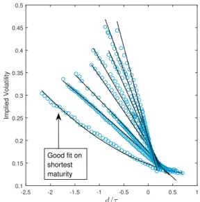
While SV FOE captures the linear d/τ properties of the data (Figure 1a), SV SOE offers a superior fit due to the inclusion of quadratic d/τ terms. In particular, it improves the fit at short maturities where skew convexity is highest (Figure 1b). Over the entire data time frame, the reduction in relative fit error SOE provides can be observed in Figure 2. A similar reduction in relative fit error can be seen for LSV (Figure 3), with the d-quadratic SOE fit (Figure 1d) offering more flexibility than a d-linear FOE fit (Figure 1c) that is not even τ-dependent in its d-slope. SOE improvements for both models justify our motivation to provide a computationally tractable and stable estimation of SOE market parameters Φ∗, seeking their associated Θ∗ fit quality.
Between the two models, from Figure 2 and Figure 3 we notice the SOE fit for LSV is inferior to SV. This shows, at least empirically, that the LSV model needs higher-order expansions than the SV model to express the extra complexity assumed by its partly-local dynamics into a tight fit of the volatility surface. Also, the LSV FOE fits are inferior to the SV FOE fits. The latter observation confirms that SOE does not act as a minor correction for LSV, and there is no explicit magnitude separation between the terms of the two expansions. For this reason we can not reuse the LSV FOE for SOE fits. Finally, in all long-term plots, we have relative fit error spikes during the indicated (light red) market distress periods, corresponding to likely spikes/instability in market parameters Φ∗.
An additional consideration that is specific to the SV model small-, small-δ regime is whether the theoretical fit accuracy scaling between FOE and SOE is explained by numerical fit errors. A tight theoretical error bound on FOE (see [8], p.145) is given byEF OE =O(+δ), while from(2)(proved in [9]) we haveESOE=O(1+q/2+
√ δ+δ√+δ3/2), ∀q <1.Therefore ESOE <O(( √ + √ δ) +δ(√+ √ δ)) =O(+δ)·O(√+ √ δ) =EF OE·O( √ + √ δ).
Figure 2shows the daily relative error fit for SOE as 40% on average of the same FOE error. For example, O(√+√δ) = 40% in the case of =δ = 0.04, matching the small-, small-δ regime assumptions. This shows that the accuracy order scaling of SV SOE vs. FOE is justified by average relative fit errors across the 2000−2011 dataset we consider.
4.3. Parameter Stability. A desirable empirical property of the SOE calibration schemes we introduced in section 3 is an acceptable and economically predictable Φ∗ parameter sta-bility. For both models, we expect more parameter instability around major observable eco-nomic/market crashes. For the SV model, we expect Φ∗ parameter values centred close to 0 as conditioned by the small-, small-δ model regime, particularly a leading magnitudeσ∗ and lowest magnitude A, B, C and φ parameters. The LSV model, in contrast, requires no pa-rameter/expansion order magnitude scaling or explicit centering conditions and all its market parameters have functional interpretations as either sensitive derivatives w.r.t model factors or direct functions of model variables. Due to this and also due to relatively larger SOE fit error than in the SV case, we expect slightly more unstable parameters than for the SV model. However, a reasonable degree of parameter stability should be expected for the LSV class as well. This expectation follows because the LSV model class represents a generalization of widely used and studied models that should capture most data variation via their dynamics rather then via parameter variation/instability over time.
Figure 1: Fitted S&P 500 index implied surface from March 18, 2010. Each straw of volatility data points corresponds to one contract maturity, with maturities increasing clockwise.
d/τ -2.5 -2 -1.5 -1 -0.5 0 0.5 1 Implied Volatility 0.1 0.15 0.2 0.25 0.3 0.35 0.4 0.45 0.5 Not fitting shortest maturity
(a) SV FOE, avg. relative fit error 6.70%.
d/τ -2.5 -2 -1.5 -1 -0.5 0 0.5 1 Implied Volatility 0.1 0.15 0.2 0.25 0.3 0.35 0.4 0.45 0.5 Good fit on shortest maturity
(b) SV SOE, avg. relative fit error 2.32%.
d -2 -1.5 -1 -0.5 0 0.5 1 Implied Volatility 0 0.1 0.2 0.3 0.4 0.5 0.6
(c) LSV FOE, avg. relative fit error 11.52%.
d -2 -1.5 -1 -0.5 0 0.5 1 Implied Volatility 0.05 0.1 0.15 0.2 0.25 0.3 0.35 0.4 0.45 0.5
(d) LSV SOE, avg. relative fit error 6.57%.
4.3.1. SV Calibration. We justify our iterative approach presented in subsection 3.1 by showing that a direct FOE reuse and no iteration on l1 can lead to unstable SOE market
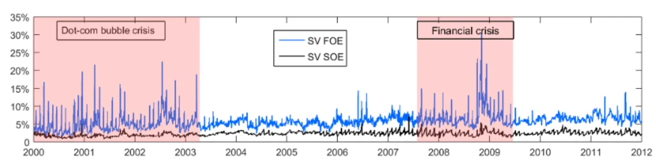
parameters. In Figure 4 we show the time evolutions of market parameters σ?, V0δ,V1δ, V3 obtained from a direct FOE calibration(7)daily during 2000-2011. All four parameters have stable evolutions with spikes occurring in crisis periods marked by abnormally high volatility spikes, such as the dot-com bubble stock market crashes within 2000-2003, and the late 2008-2009 financial crisis. However, looking closely at what happens in any of these periods, for
Figure 2: SV FOE vs. SOE daily % avg. relative fit error on 2000-2011 data. FOE average error is 5.79%, while for SOE it is 2.28%, a ≈60% reduction.
Figure 3: LSV FOE vs. SOE daily % avg. relative fit error on 2000-2011 data. FOE average error is 9.80%, while for SOE it is 6.08%, a ≈40% reduction.
example the dot-com bubble during 2000-2001, we can see inFigure 5 that parameterVδ 0 has
minor spikes diverting from its long-run positive mean to negative values, approaching and crossing parameter V1δ in the process. The functional form of SOE parameters B2δ,V
0δ 1 σ0 , V0δ 0 σ0 in (20) depends on terms V0δ and V0δ +V1δ at denominator level. As a consequence, as
Figure 6 illustrates, parameter B2δ for instance will become unstable when the denominator terms V0δ,V0δ+V1δ approach 0 during market crises or when 1-month options are very close to expiry (order of a few days). A possible solution to parameter numerical issues on data from volatility spike periods (see Figure 5) is to impose explicit constraints on V0δ and V1δ in the FOE calibration (7).
However, we recognize that V0δ, V1δ are in fact residual, smaller parameters in FOE of magnitude order √δ and the volatility zeroth-order approximation σ? is the leading order parameter that governs their evolution (as required by the model asymptotic regime and as evidenced empirically inFigure 4). Furthermore, σ? also impacts extensively Φ1 parameters
as a denominator to the majority of terms in equations (4). Therefore, an overfit inσ? from d/τ-linear FOE can significantly impact the stability and ranges of the new parameters Φ1
introduced via SOE. To mitigate a potential overfit inσ? impacting all parameters in Φ either directly or via FOE parameters, the corrective measure we impose is to iterate over σ? as a volatility proxy parameter (0%−100%). Afterwards, we find the optimalσ∗ value minimizing kΦ∗(σ∗)k2(minimizing parameter ranges and therefore instability), where each Φ∗is a function
of fixed σ∗ and parameters V0δ, V1δ, V3 are determined from FOE calibration with fixed σ∗. Since in(7),l1 =σ?+
V
3
Figure 4: SV FOE market parameters calibrated for data from 2000-2011.
03-Jan-2000 25-May-2000 17-Oct-2000 13-Mar-2001 03-Aug-2001 31-Dec-2001
-0.1 -0.05 0 0.05 Vδ 1 Vδ 0
Figure 5: SV FOE parametersV1δ vsV0δ.
be fixed and iterated over directly in the FOE calibration, effectively leading to an iteration overσ?. Since there are three FOE coefficientsm1, p1, q1 left to regress on, we fit them to the
data across all maturities at once not maturity-by-maturity as described in [8]. For each fixed l1, we find the remaining coefficients via the adapted FOE calibration procedure, afterwards
translating them into values for σ∗, V0δ, V1δ, V3. Finally, over all l1 iterations, we choose the
optimal Φ∗ as the minimal l2-norm set among Φ∗(l1) (as in the original formulation (6)).
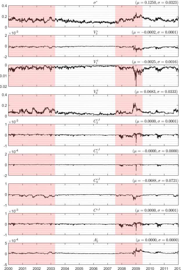
Following the SOE calibration procedure insubsection 3.1, numerical results show a trans-lation of the stable coefficient set Θ∗(Figure 8) into a stable market parameter set Φ∗(Figure 9
03-Jan-2000 25-May-2000 17-Oct-2000 13-Mar-2001 03-Aug-2001 31-Dec-2001 -20 0 20 40 B δ 2
Figure 6: B2δ parameter throughout 2000-2001 for direct SV FOE reuse.
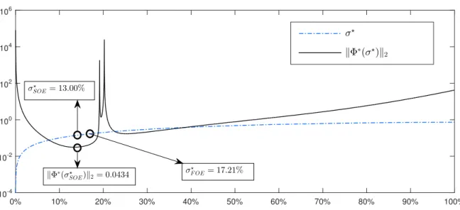
0% 10% 20% 30% 40% 50% 60% 70% 80% 90% 100% 10-4 10-2 100 102 104 106 σ⋆ kΦ∗(σ⋆)k2 σ⋆ F OE= 17.21% σSOE⋆ = 13.00% kΦ∗(σ⋆SOE)k2= 0.0434
Figure 7: SV kΦ∗(σ∗)k2 vs. σ? for data from March 18, 2010. y axis is on logarithmic scale.
andFigure 10). All parameters have time series centred around 0 and are limited to a range of [−1,1], withσ?a leading order parameter, as expected. The values ofσ? as a SOE parameter (Figure 9) are in line with, but noticeably smaller than as a FOE parameter (Figure 4). To understand this deviation, that is also the root cause of direct FOE use yielding unstable SOE parameters, we look at kΦ∗(σ∗)k2 for different values of σ? as l1 is iterated (l1 ≈ σ? as V3
is very small comparatively). As Figure 7 illustrates, the σ? obtained for kΦ∗k2 is a slight under-estimator of the same parameter obtained directly from FOE. On the test day March 18, 2010 we have σF OE? −σ?SOE = 4.21%, and the gap between the two is moderate across time, with slight increases in periods of market stress. Intuitively, becauseσ? appears in linear form in residual regression terms l1 in FOE and l in SOE, it decreases when going from a
coarser FOE model to a finer SOE model as the extra 14 market parameters can convey more accurately the extra implied volatility surface information. It is also important to note that the non-convexity of kΦ∗(σ∗)k2 as a function of σ∗ inFigure 7does not impose problems, as we exhaustively iterate in a fine-grained fashion overσ?. Additionally, due to the fact thatσ? is a leading-order parameter in the vector Φ, whenσ? varies infinitesimally,kΦ∗(σ∗)k2 cannot
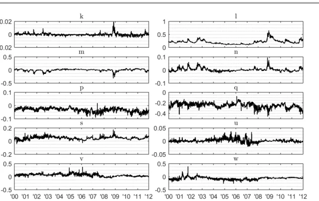
Figure 8: SV Θ∗ calibrated for 2000-2011 data.
jump locally. Moreover, the stability of σ? over multiple days is supported by the fact that σ? is linearly coupled to an empirically stable estimated parameterl (see Figure 8), and the additional terms inl are small in magnitude in the model regime.
We also observe how V0δ, V1δ are well separated in Figure 9, with V0δ pushed to positive values compared to FOE (Figure 4), which naturally leads to stable parameters B2δ,V10δ
σ0 , V0δ
0
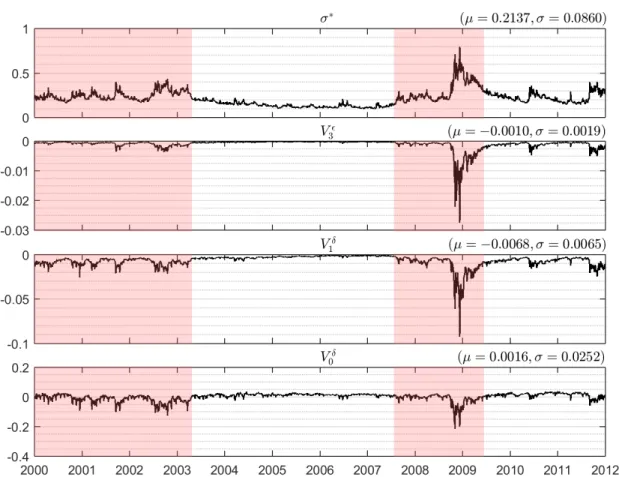
σ0 . The parameterV00δ/σ0 varies most during calm market periods (such as 2003-2008) capturing daily data variation as its multiplicative factorsV0δ, V1δ from(4)are very stable. All other Φ∗ parameters vary most in market stress periods, most noticeably during the financial crisis, as expected.
Furthermore, we expect the parameter φ to have a relatively higher frequency variation due to being the only parameter in Φ∗ directly dependent on the SV model fast factorY (see
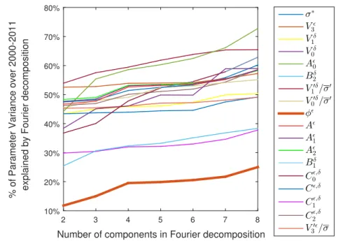
(8)). To explain the variation frequency of time series 2000−2011 for all Φ∗parameters shown inFigures 9to10, we perform Fourier decompositions on all time series allowing the number of components used to vary from 2 to 8. To be more precise, letX(t) denote the relevant time series, then we attempt to decompose it as follows,
F(t) =a+bt+ N X
j=0
cjcos(2πφjt+lj), t∈[0, T],
whereN is the number of components in the decomposition. In our case N ranged from 2 to 8. The harmonics of the equation above are obtained from the peaks of the Fourier transform of the data, and the other coefficients are obtained from a least squares regression, i.e. by
Figure 9: SV Φ∗calibrated for 2000-2011 data. The light red areas represent periods of market distress overlapping with higher parameter variability.
Figure 10: (cont.) SV Φ∗ calibrated for 2000-2011 data. The light red areas represent periods of market distress overlapping with higher parameter variability.
Number of components in Fourier decomposition
2 3 4 5 6 7 8
% of Parameter Variance over 2000-2011 explained by Fourier decomposition
10% 20% 30% 40% 50% 60% 70% 80% σ∗ Vǫ 3 Vδ 1 Vδ 0 Aǫ 0 Bδ 2 V′δ 1 /σ′ V′δ 0 /σ′ φǫ Aǫ Aǫ 1 Aǫ 2 Bδ 1 C0ǫ,δ Cǫ,δ C1ǫ,δ C2ǫ,δ V′ǫ 3/σ
Figure 11: Variance explained by Fourier decompositions with 2-8 components for all SV Φ∗ time series (2000-2011). Each added componenti(i∈2,8) has frequency proportional toi. minimizingkX(t)−F(t)k2. We used standard techniques to perform the analysis, the precise
methodology is described in Chapter 13 of [1]. By extracting the percentage of total variance explained by the Fourier decompositions with a fixed number of components,Figure 11shows that the variance for φ is not adequately captured even when using eight components of increasing frequencies. It is clear fromFigure 11that there is a qualitative difference between φand the rest of the Φ∗ parameters. Therefore,φhas a relatively higher frequency variation and needs more Fourier components of higher frequency to capture it, as expected by its direct dependence onY.
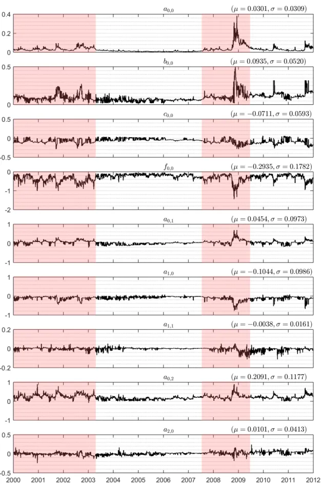
4.3.2. LSV Calibration. Parameters η0,0,∀η ∈ {a, b, c, f}, appearing in (13), represent
derivative-free parameters and have a direct interpretation in terms of model variables from
(12). In particular, b0,0 is a function of σ1, which represents the percentage volatility of the
second model factor Y; f0,0 =µ1 represents the percentage drift of Y; c0,0 is the product of
the two factors volatilitiesσ0, σ1 and the correlation ρ. Given that σ0 can be found directly
from Θ∗ then fixing σ1, µ1, ρ as percentage values fully determines b0,0, c0,0, f0,0. Since σ1 is
the volatility of the additional factorY and therefore positive, we bound it within [0,2.5] (not just [0,1] in order to accommodate potential spikes in market stress periods). Accounting for
Remark 2 we iterate f0,0 = µ1 over [−2.5,0] and let ρ be fixed as a correlation percentage
necessarily bounded by [−1,1], inducing an iteration overc0,0. InFigure 16, we notice over the
entire time period 2000-2011 we have kΦ∗k2 <max(b20,0, f02,0) = max(2.54/4,2.52), validating our chosen bounds, since any wider bounds would result in a kΦk2 > kΦ∗k2. We choose to iterate numerically in 1% increments over σ1, µ1, and 10% increments over ρsince its impact
0 0.5 1 l -1 -0.5 0 q -1 0 1 m -0.5 0 0.5 n '00 '01 '02 '03 '04 '05 '06 '07 '08 '09 '10 '11 '12 -1 0 1 w '00 '01 '02 '03 '04 '05 '06 '07 '08 '09 '10 '11 '12 0 0.2 0.4 s
Figure 12: LSV Θ∗ calibrated for 2000-2011 data.
on any of b0,0, c0,0, f0,0 occurs for b0,0 when σ1 = 2.5 and a 1% increment in σ1 increases
b0,0 = σ12/2 by ≈ 2.5%. The previous extreme case of a b0,0 increment of 2.5% is likely to
happen only in very unstable market conditions with high volatility in both factors, and is in line in magnitude with daily variations forb0,0 seen in Figure 13 where the iteration scheme
described here was used. Therefore, any possible jumps in parameters Φ∗ due to using lower increments is in the order of or below one-day parameter variations. Obviously a finer grained numerical search over b0,0, c0,0, f0,0 will likely improve stability of Φ∗ further and should be
preferred, but in order to achieve the computational efficiency necessary for a multi-year data study, we compromised on numerical accuracy to an acceptable level of empirical stability. The choices we made are similar to any automatic numerical solver iterating on b0,0, c0,0, f0,0 and
possibly also a0,1 (we find a0,1 explicitly motivated by it being an unbounded Y-derivative
parameter), except we use additional model-dependent numerical insights unavailable to a solver.
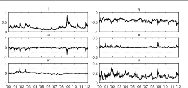
We follow the LSV calibration scheme insubsection 3.2with the numerical choices intro-duced earlier. The Φ∗ values we obtain in Figure 13and Figure 14given fitted coefficients in
Figure 12show reasonable stability with more prominent variation in market distress periods, as expected.
An important point related to the sign symmetry explained in Remark 2 is that any sign choice for one of a0,1, a1,1, c0,0, c1,0, f0,0, f1,0 is related to choosing more specific model
dynamics and directly impacts stability due to enforcing one parameter sign, one example being SABR dynamics underf0,0<0 as explained inRemark 2. The parameter sign symmetry
we identified indicates that the model class introduced in subsection 2.2 presents a generic formulation inclusive of a wide array of more specific model dynamics, where a specialized choice of one parameter sign is needed in its second order expansion calibration.
Figure 13: LSV Φ∗ calibrated for 2000-2011 data. The light red areas represent periods of market distress overlapping with higher parameter variability.
Figure 14: (cont.) LSV Φ∗calibrated for 2000-2011 data. The light red areas represent periods of market distress overlapping with higher parameter variability.
4.3.3. Norms Comparison. Since both Θ∗ and Φ∗ express the same fit quality and there-fore implied surface information as different parameter sets, we expect them to have compa-rablel2-norms. For the SV case, we have an increase of only 55% on average inkΦ∗k2 relative
to FOE market parameters norm and a 40% reduction on average from kΘ∗k2 tokΦ∗k2 (see Figure 15). For the LSV case, the two norms kΘ∗k2 and kΦ∗k2 are comparable, with a 20%
increase on average for kΦ∗k2 (see Figure 16). These results confirm the robustness of the proposed SOE calibrations in obtaining anl2-minimal Φ∗ set comparable inl2-norm with Θ∗.
5. Discussion. We proposed iterative algorithms for the problem of finding SOE market parameters Φ∗ given the coefficient set Θ∗ in the calibration of both multi-scale SV models studied in [8,9] and LSV models studied in [14]. Our solution takes advantage of analytical structures in the inversion problem from coefficients to market parameters. For both model classes, this involves multiple parameter reductions leading to reformulations and analytical derivations within the non-linear algebraic minimization problem of finding a minimall2-norm
Φ∗. Our approach leaves only a minor subset of Φ∗ to be determined numerically. In the SV case, we make use of the higher order magnitude scaling of first order perturbation expansion (FOE) parameters, recognizing their impact on the finer grained second order expansion (SOE) parameters, and exploit this to iterate over a single most significant market parameter. In the LSV case, we restrain the iteration to interpretable derivative-free market parameters that
Figure 15: SV l2-norms for FOE market parameters, Θ∗ and Φ∗, with averages of 0.0539,
0.1323 and 0.0830, respectively.
Figure 16: LSV l2-norms for Θ∗ and Φ∗, with averages of 0.2782 and 0.3311, respectively.
can be easily bounded. Our methods therefore provide the computational tractability needed to successfully calibrate successive implied volatility expansions in their more accurate SOE form in practice.
Our proposed methods are also tested and validated numerically on extensive real S&P 500 index options data, taking advantage of the better SOE fit while showing the parameter stability properties expected from a robust model calibration solution. Despite the sharp parameter number increase when going from FOE to SOE (from 4 to 18 for SV, from 5 to 13 for LSV), stability properties and, in the SV case, the asymptotic assumptions of small parameters are still met. Moreover, to our knowledge, this paper also provides a first extensive numerical analysis of the calibration and parameter stability offered by model classes with explicit successive implied volatility expansions while taking advantage of their structure.
We believe the results are encouraging for the use of both multiscale stochastic and local-stochastic volatility models in practice in a tractable way, even in higher order perturbation expansions. The parameter reductions (by grouping or gradients), lower order expansion reuse or restricted iteration approaches that we employed can potentially be used in the calibration of more sophisticated third order implied volatility expansions or more generally, in other model calibrations inducing explicit successive implied volatility expansions. Calibrated SOE market parameters Φ∗ from the European options volatility surface can also be used to speed up Monte Carlo simulations for the pricing of other exotic option contracts using similar ideas to those in [8]. Finally, owing to SOE calibration accuracy and stability especially for SV, the market parameter set can be used as a short-term predictive parametrization of implied volatility surfaces, the primary objective of econometric volatility models [3].
Acknowledgements. The authors thank the editors and anonymous referees for their helpful comments on earlier versions of the paper. Radu Baltean-Lugojan’s work was sup-ported by EPSRC DTP funding. The work of the second author was partially supsup-ported by EPSRC grants EP/M028240, EP/K040723 and an FP7 Marie Curie Career Integration Grant (PCIG11-GA-2012-321698 SOC-MP-ES).
REFERENCES
[1] J. Cryer and K. Chan,Time Series Analysis, With Applications in R, Springer, 2008.
[2] B. Dumas, J. Fleming, and R. Whaley,Implied volatility functions: Empirical tests, The Journal of
Finance, 53 (1998), pp. 2059–2106.
[3] R. Engle and A. Patton,What good is a volatility model, Quantitative finance, 1 (2001), pp. 237–245. [4] S. Figlewski,Estimating the implied risk neutral density, Volatility and time series econometrics: Essay
in honor of Robert F. Engle, Tim Bolloerslev, Jeffrey R. Russell, Mark Watson, (2008).
[5] J. Fouque and C. Han,Asian options under multiscale stochastic volatility, Contemporary Mathematics, 351 (2004), pp. 125–138.
[6] ,Variance reduction for monte carlo methods to evaluate option prices under multi-factor stochastic
volatility models, Quantitative Finance, 4 (2004), pp. 597–606.
[7] J. Fouque, G. Papanicolaou, R. Sircar, and K. Solna,Short time-scale in s&p500 volatility, Journal of Computational Finance, 6 (2003), pp. 1–24.
[8] ,Multiscale Stochastic Volatility for Equity, Interest Rate, and Credit Derivatives, Cambridge
Uni-versity Press, 2011.
[9] J.-P. Fouque, M. Lorig, and R. Sircar, Second order multiscale stochastic volatility asymptotics:
stochastic terminal layer analysis and calibration, Finance and Stochastics, (2016), pp. 1–46. [10] J. Gatheral,The volatility surface: a practitioner’s guide, vol. 357, John Wiley & Sons, 2011.
[11] P. S. Hagan, D. Kumar, A. S. Lesniewski, and D. E. Woodward,Managing smile risk, The Best
of Wilmott, (2002), p. 249.
[12] C. Homescu, Local stochastic volatility models: calibration and pricing, Available at SSRN 2448098,
(2014).
[13] M. Joshi,The concepts and practice of mathematical finance, vol. 1, Cambridge University Press, 2003. [14] M. Lorig, S. Pagliarani, and A. Pascucci,Explicit implied volatilities for multifactor local-stochastic
volatility models, Mathematical Finance, (2015), pp. n/a–n/a.
[15] L. Merville and D. Pieptea, Stock-price volatility, mean-reverting diffusion, and noise, Journal of
Financial Economics, 24 (1989), pp. 193–214.
[16] U. Muller, M. Dacorogna, D. Rakhal, R. Olsen, O. Pictet, and J. von Weizsacker,Volatilities
of different time resolutions – analyzing the dynamics of market components, Journal of Empirical
Finance, 4 (1997), pp. 213–239.
[17] OptionMetrics, IvyDB US File and Data Reference Manual Version 3.0, downloadable .pdf available