Sensitivity and inverse analysis methods for parameter intervals

Sensitivity and inverse analysis methods for parameter intervals

Guojian Shao1, Jingbo Su2

1_{Department of Engineering Mechanics, Hohai University, Nanjing, 210098, China} 2

College of Harbor, Coastal and Offshore Engineering, Hohai University, Nanjing, 210098, China Received 30 April 2010; received in revised form 15 June 2010; accepted 25 June 2010

Abstract: This paper proposes a sensitivity analysis method for engineering parameters using interval analyses. This method substantially extends the application of interval analysis method. In this scheme, parameter intervals and decision-making target intervals are determined using the interval analysis method. As an example, an inverse analysis method for uncertainty is presented. The intervals of unknown parameters can be obtained by sampling measured data. Even for limited measured data, robust results can also be obtained with the inverse analysis method, which can be intuitively evaluated by the uncertainty expressed in terms of an interval. For complex nonlinear problems, an iteratively optimized inverse analysis model is proposed. In a given set of loose parameter intervals, all the unknown parameter intervals that satisfy the measured information can be obtained by an iteratively optimized inverse analysis model. The influences of measured precisions and the number of parameters on the results of the inverse analysis are evaluated. Finally, the uniqueness of the interval inverse analysis method is discussed.

Key words: interval analysis method; sensitivity analysis; reversible inverse analysis method; iteratively optimized inverse analysis method

1 Introduction



The purpose of a sensitivity analysis is to evaluate the extent of the changes that occur in a decision- making target or output by varying one or more of the uncertain input factors. Based on such a sensitivity analysis, the enduring capability or stability of the target can be assessed and the predictions can be made regarding changes that might occur in the output when large changes happen to the input. Traditionally, sensitivity analysis methods have been proposed based on stochastic theory and fuzzy theory. However, more recently developed interval analysis methods are gaining their acceptance. However, without sufficient experimental data to generate suitable probability density functions, these traditional methods are not likely to produce sufficiently accurate results. Elishakoff [1] discussed such uncertainties.

The interval analysis method, introduced by Moore

Doi: 10.3724/SP.J.1235.2010.00274



*Corresponding author. Tel: +86-25-83787976; E-mail: [email protected] Supported by the National Natural Science Foundation of China (50978083) and the Fundamental Research Funds for the Central Universities (2010B02814)

and Yang [2], is based on non-probabilistic interval sets. This method assumes that the uncertainties of all loads and resistance parameters are bounded from above and below. By applying the interval analysis method, a sharp interval set that includes all feasible solutions can be obtained.

By far, the most widely investigated sensitivity analysis techniques include the Bayesian inverse analysis method, the maximum likelihood inverse analysis method, the Kalman filter inverse analysis method and the fuzzy inverse analysis method. For these methods, the deterministic stiffness matrix of the system is assumed to be known and the distribution of external loads is identified by interval displacements using the Lagrange multiplier method by Nakagiri and Suzuki [3]. These techniques all address the concept of interval inverse analysis, which constrains a model using the variable metric method. Such a method was used by Wang et al. [4, 5] to analyze the initial stress field, elastic constants and vibrational parameters of tunnel walls in a concrete dam. However, the model is sensitive to the initial values of the parameters, which in turn results in different initial values being used for the computation. Based on the perturbation method,

another interval inverse analysis model was proposed by Liu et al. [6] to analyze the elastic constants of the rocks in tunnel walls. The central values of the interval parameters are first determined by a conventional inverse analysis method, then the uncertainties of the interval parameters are constrained by the perturbation formulae.

In this paper, the interval analysis method is briefly outlined. The formulae needed to compute the sensitivity factors of the parameters are derived based on interval theory. A method for obtaining the parameter intervals and decision-making targets is presented. An iterative optimization model based on inverse analysis is then proposed to identify the parameter intervals. Finally, conditions needed to determine the existence or convergence of a solution are summarized.

2 Brief introduction to the interval

analysis method

An interval number is defined by bounded sets of

real numbers, which can be expressed as I

X 

[ , ] { |x x  x x x x}, where x and x are its two boundaries. The uncertainty  X (xx) / 2 , the

central value C

( ) / 2

X  xx , and the interval

number I C

[ ,

X  X  X C

]

X  X are defined. The

variation coefficient of I

X is defined by

C /

X X

   , and its absolute value is defined as

I

|X | max{| |, | x x|} (1)

For the interval vector I I I I T

1 2 {X , X , , Xn}   V , its norm is I I I I 1 2 ||V || max{| X |, |X |, , | Xn|} (2) The central value and uncertainty of _VI _are

C C C C T 1 2 {X , X , , X_n}   V (3) T 1 2 { X , X , , Xn}   V    (4) It is assumed that I I I I T 1 2 { X , X , , Xn} V      (5) where I [ , ]( 1, 2, , ) i i i X X X i n       . Thus, I V C  I

V V . Similar expressions exist for an nn

interval matrix _AI _{, and its central value and}

uncertainty are C ₍ C₎ ij a  A ,   A ( a_ij) (6) Therefore, we have _AI_AC _AI , where  _AI I {aij}, I [ , ] ij ij ij a a a     .

For the interval numbers I

[ , ]

X  x x and

I

[ , ]

Y  y y , the basic operations are

I I I I I I I I [ , ] [ , ] [ , ] [ , ] [ , ] [ , ] [ , ][ , ] [min{ , , , }, max{ , , , }] 1 1 / [ , ] / [ , ] [ , ] , (0 [ , ]) X Y x x y y x y x y X Y x x y y x y x y X Y x x y y x y xy xy x y x y xy xy x y X Y x x y y x x y y y y               _    _      _      _   _    (7) According to the basic operations presented above, we can find that the commutative and associative laws for addition and multiplication hold true. However, other operation laws (such as the distributive and counter-balance laws) present the inclusive forms, e.g.

I₍ I I₎ I I I I

X Y Z X Y X Z

Detailed interval computations are shown in Refs.[7, 8]. The interval operations may result in interval extension[9]. We can guarantee a sharp interval by the perturbation method [10]. Some other methods have been brought forward to deal with interval extensions,

such as combination monotone method [11] and

truncation method [11, 12].

The interval finite element method (FEM) is based on a combination of the interval analysis method and a traditional FEM. The response intervals of a linear-elastic beam were solved using triangle inequality and linear programming [13]. The interval-truncation approach was proposed to limit the interval extension for realistic and accurate solutions [11]. Based on perturbation theory, the interval matrix perturbation method and the interval parameter perturbation method were proposed to estimate the static displacement bounds of structures with interval parameters [10, 14, 15]. Considering the interactions among uncertain parameters, an improved interval perturbation method was proposed [16]. Based on some of the properties and operation laws of the interval number, a static governing equation for an

n-freedom uncertain displacement field was

transformed into (2n)-order linear equations [17]. Starting from the elements, the interval parameter perturbation method was proposed for the response intervals of a linear-elastic beam [18], and the sub-interval perturbed finite element method was proposed and applied to anti-slide stability analysis

276 Guojian Shao et al. / Journal of Rock Mechanics and Geotechnical Engineering. 2010, 2 (3): 274–280

[19]. More recently, the dynamic responses of uncertain structures with interval parameters have been widely investigated [20, 21].

3 Parameter sensitivity interval

analysis method

3.1 Sensitivity factor matrix

For a structure with n model parameters [22], the parameter vector is defined as V { ,x₁ x₂,, x_n}, where x_j= [x_j, x_j](j1, 2,, n). In addition, the decision-making target vector Y { ,y₁ y₂,, y_m} is

composed of m decision-making targets, where

i

y = [ ,y_i y_i] (i1, 2,, m). Because one model parameter vector V must correspond to one decision- making target vector Y, the mapping of VY is established and the relationships between x_j and y_i

are given by 11 1 12 2 1 1 1 21 1 22 2 2 2 2 1 1 2 2 n n n n m m mn n m m y x x x y y x x x y y x x x y                      _         _     (9) where _ij (i1, 2,, m; j1, 2,, n) is the integrative influence factor of the j-th model parameter on the i-th decision-making target. If VY is nonlinear, then 1 1 1 2 2 2 1 2 1 2 ( , , , ) ( , , , ) ( , , , ) n n m m n y y x x x y y x x x y y x x x     _     _     (10)

Applying the first-order Taylor series, we obtain

c c c c c c c c c c c c c c 1 1 1 1 1 1 2 2 1 2 c 1 c c 2 2 2 2 1 1 2 2 1 2 c 2 c c 1 1 2 2 1 2 c ( ) ( ) ( ) ( ) ( ) ( ) ( ) ( ) ( ) n n n n n n m m m m m n n n y y y y x x x x x x y x x x y y y y x x x x x x y x x x y y y y x x x x x x y x x x             _                            _      V V V V V V V V V V V V                        (11) i.e. c c c 11 1 12 2 1 1 1 c c c 11 1 12 2 1 1 2 21 1 22 2 2 2 c c c 21 1 22 2 2 2 1 1 2 2 c c c 1 1 2 2 ( ) ( ) ( ) n n n n n n n n m m mn n m m m m mn n m y x x x y x x x y y x x x y x x x y y x x x y x x x y                                _       _{ }      _                        V V V (12) where c i ij j y x    V , c c c c 1 2 { ,x x , , xn}   V . Because of

the difference in the dimensions of the model parameter, it is very difficult to determine ij. Thus

the influence of a single model parameter on a certain decision-making target is of concern.

Given the boundary influence value interval of the model parameter xj[xj, xj] (j1, 2, , )n and the

decision-making target _, , [ , ] i _{i j} i j y  y y (i1, 2, , m), where _, , [ , _{i j}] i j y y is one subset of [ , ]_i i y y , the

following parameter is defined:

, _,

( ) / ( )

ij yi j y_{i j} yi y_i

     (13) where _ij is the independent influence factor of the model parameter

x

i

y. Because _,

,

[y_{i j}, yi j] is one subset of [ , ]y_i yi , then 0_ij1. When _ij is close to 0, this indicates that the model parameter x_j has almost no influence on the decision-making target. On the contrary, when ij

is close to 1, the model parameter x_j has a very significant influence on the decision-making target y_i. Therefore, the sensitivity factor matrix  of model parameter is described by 11 12 1 21 22 2 1 2 n n m m mn                _{  }         _{  }            (14)

The influence of each model parameter on each decision-making target is different. Furthermore, the influence of the same model parameter on different decision-making targets can vary considerably. From the sensitivity factor matrix , the column vectors show the independent influence factors of each model

parameter on all the decision-making targets, the value of each factor reflects the influence of the model parameter on the corresponding decision-making target. The row vectors show the influence of all the model parameters on the same decision-making target: the larger the values of _ij are, the greater the influence of the model parameters is. The sensitivity analysis method, to some extent, can consider the inter- relationship of the model parameters.

3.2 Determination of the boundary influence value interval and decision-making target interval

The boundary influence value interval _,

, [ , _{i j}]

i j

y y

of the model parameter xj on decision-making target i

y can be investigated by interval finite element

optimization analysis when x_j is an interval number but the other parameters are assumed to be constant and equal to the interval medium-values.

The decision-making target interval [ , ]_i i

y y can be

determined using a similar method when all the parameters adopt interval numbers.

3.3 Discussion on parameter intervals

During the sensitivity analysis, the difference of the parameters’ dimensions may induce a variance in the sensitivity degree. Therefore, the parameters’ dimensions must be identified or the parameters must be transformed to some extent, as illustrated by the following example. Given 2 10 zx  y , where I xX , I yY , I zZ , _XC_YC_{10. z is a binomial function of}

x, but a simple function of y, so the dimensions of

x and y are different. If _x_y0.1, we can get

I

[9, 11]

X  , I

[9, 11]

Y  . By interval operation, the

decision-making target interval I

[171, 231]

Z  is

obtained, as are the boundary influence value intervals of parameters x and y on the decision-making target

z. These are [181, 221] and [190, 210], respectively. Therefore, the sensitivity factors _zx and _zy are 2/3 and 1/3, respectively; the sensitivity of parameter x

is greater than that of parameter y for the same

decision-making target. If x 0.1 and y 0.3, the

sensitivity factors _zx and _zy are 4/9 and 5/9, respectively. Here, the sensitivity degree of parameter

x to the decision-making target z is less than that of parameter y. If _x _y 0.01, the same conclusion,

0.1

x y

   , can be made. It can be stated that

different coefficients of variation can result in different sensitivity factors of the model parameters to the decision-making target. When the same coefficients of variation are used, the same sensitivity factors are

desired.

Thus, to obtain the sensitivity factor matrix , the parameter intervals must be determined using the same coefficient of variation  and parameter medium-

value C

X .

4 Iterative optimization of the

inverse analysis model

For complex nonlinear problems, when the forward convergence condition is not satisfied, the interval reversible inverse analysis model does not work well.

Considering the uncertainty, the unknown parameter vector is denoted as I

. For practical engineering problems, a loose parameter vector I

p

 can be set by engineering experience, testing information, exploration data, and so on. This may ensure that the solution of the inverse problem is in accordance with actual physical concepts and geological data. If the

measured displacement is taken to be I

f

U , the

following inverse analysis model can be proposed for the interval parameter vector I

by the optimization method: I p I cal f for min / max ( 1, 2, , ) s.t. ( , ) ( ) i i m            _   _ K U U = R U U     

where U_cal is the calculated displacement by

( , )  ( )

K  U U R . Therefore, we have

I 



1 1 2 2

{[min( ), max()], [min( ), max( )], ,

T

[min(_m), max(_m)]} (16) Equation (15) is sensitive to the initial values of the parameters. For comparison, different initial values are used [6]. Thus, an iterative optimization of the inverse analysis model is proposed as follows:

(1) Step 1. Select one initial parameter vector ₀ I

0 p

(  ). Here, I

cal f

U U and Ucal are computed

by K(0, U U) R(0).

(2) Step 2. Compute I

0

 by the following

278 Guojian Shao et al. / Journal of Rock Mechanics and Geotechnical Engineering. 2010, 2 (3): 274–280 0 I 0 p 0 0 I cal f for min / max ( 1, 2, , ) s.t. ( , ) ( ) ( 1, 2, , ; ) i i i k k i m k m k i              _   _        _ K U U R U U     (17) Therefore, we have I 0  10 10 20 20

{[min( ), max( )], [min( ), max( )],,

T

0 0

[min(_m ), max(_m )]} (18) (3) Step 3. Assume the parameter vector of step t is

I

t

 , the parameter vector of step t+1 can be gained by

( 1) 1 1 I ( 1) p I ( 1) I cal f for min / max ( 1, 2, , ) s.t. ( , ) ( ) ( 1, 2, , ; ) i t t t i t i k t kt i m k m k i                   _            _ K U U R U U     (19) Therefore, we have I +1 t   {[min(1( +1)t ), max(1( +1)t )], 2( +1) 2( +1) [min( t ), max( t )], , T ( +1) ( +1) [min(_{m t} ), max(_{m t} )]} (20) (4) Step 4. After obtaining the final parameter vectors by an iterative optimization process, the convergence condition of the iterative optimization can be defined by the following vector norm:

I I 1

t  t 

  (21) where || || is the interval vector norm, and  is a small parameter. If the norm is a Eucledian norm, then

2 2 I I 1 1 1 2 2 t  t  t  t  t  t      

During the process of convergence, the final intervals of unknown parameters gradually approach the exact results. So the process is actually a naturally converging one. Genetic algorithms have powerful

capabilities in global searches and limited capabilities in local searches; however, simulated annealing algorithms have powerful local search capabilities and limited capabilities in global searches. Therefore, for rapid and correct convergence, genetic and simulated annealing algorithms are used together for the optimization.

5 Numerical example

To demonstrate the applications of the proposed method, and to estimate the effect of measured precisions on analysis results, a tunnel excavation example is considered.

The simulation involves a tunnel with a horseshoe cross-section that is 7.8 m wide and 9.0 m high. The intervals of unknown parameters (cohesion force c, friction angle , Young’s modulus E and Poisson’s ratio ) are analyzed using the iterative optimization of an inverse analysis model. The computation zone is divided into a mesh consisting of 488 plane strain elements and 485 nodes (Fig.1); and the boundaries have normal constrains. A Drucker-Prager constitutive model is employed to simulate rock behavior.

Fig.1 The finite element meshes.

According to the geological exploration data, field and laboratory tests, and expert opinion, the loose intervals of unknown parameters were adopted as follows: 0.2 MPa c 0.7 MPa, 2739, 1.3 GPa E 6.0 GPa, 0.30  0.35.

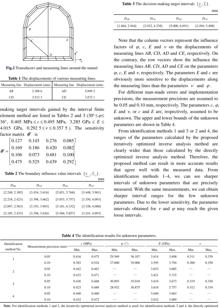
The transducers and measuring lines around the tunnel are shown in Fig.2. The central value vector of the parameters { , , , }c  E  {0.45 MPa, 33, 3.65 GPa, 0.325}. The displacements of the measuring lines are shown in Table 1.

The coefficient of variation is taken as 0.1. The boundary influence value intervals and the

decision-Fig.2 Transducers and measuring lines around the tunnel.

Table 1 The displacements of various measuring lines.

Measuring line Displacement (mm) Measuring line Displacement (mm)

AB 2.306 6 AD 5.699 2

CD 3.512 3 CE 3.672 1

making target intervals gained by the interval finite element method are listed in Tables 2 and 3 (30 36, 0.405 MPa c 0.495 MPa, 3.285 GPa  E 

4.015 GPa, 0.292 5  0.357 5). The sensitivity factor matrix  is 0.127 0.145 0.276 0.085 0.169 0.186 0.420 0.082 0.106 0.073 0.681 0.100 0.475 0.525 0.439 0.292        _{ }     

Table 2 The boundary influence value intervals [y_{i j,},yi j, ].

mm DAB DCD DAD DCE [2.248, 2.385] [3.434, 3.616] [5.651, 5.766] [3.448, 3.961] [2.218, 2.423] [3.398, 3.662] [5.653, 5.757] [3.350, 4.093] [2.097, 2.563] [3.193, 3.903] [5.181, 6.332] [3.338, 4.080] [2.185, 2.433] [3.398, 3.636] [5.566, 5.857] [3.241, 4.093]

Table 3 The decision-making target intervals [ ,y y_i i]. mm

DAB DCD DAD DCE [1.864, 2.944] [2.922, 4.338] [5.000, 6.691] [2.494, 5.408]

Note that the column vectors represent the influence factors of , c, E and  on the displacements of measuring lines AB, CD, AD and CE, respectively. On the contrary, the row vectors show the influence the measuring lines AB, CD, AD and CE on the parameters , c, E and , respectively. The parameters E and c are obviously more sensitive to the displacements along the measuring lines than the parameters  and .

For different man-made errors and implementation precisions, the measurement precisions are assumed to be 0.05 and 0.10 mm, respectively. The parameters c, ,

E and , or c and E are, respectively, assumed to be unknown. The upper and lower bounds of the unknown parameters are shown in Table 4.

From identification methods 1 and 3 or 2 and 4, the ranges of the parameters calculated by the proposed iteratively optimized inverse analysis method are clearly wider than those calculated by the directly optimized inverse analysis method. Therefore, the proposed method can result in more accurate results that agree well with the measured data. From identification methods 1–4, we can see sharper intervals of unknown parameters that are precisely measured. With the same measurements, we can obtain sharper interval ranges for the few unknown parameters.Due to the lower sensitivity, the parameter intervals obtained for  and  may reach the given loose intervals.

Table 4 The identification results for unknown parameters.

c(MPa) _{( )}o _{E(GPa) }

Identification

method No. Measurement precision (mm) Min. Max. Min. Max. Min. Max. Min. Max.

0.05 0.416 0.475 29.569 36.107 3.614 3.698 0.311 0.339 1 0.10 0.383 0.524 27.000 39.000 3.595 3.794 0.300 0.350 0.05 0.442 0.461 — — 3.633 3.685 — — 2 0.10 0.433 0.471 — — 3.621 3.715 — — 0.05 0.436 0.468 30.893 35.018 3.634 3.673 0.319 0.330 3 0.10 0.423 0.489 28.932 36.875 3.618 3.757 0.312 0.334 0.05 0.440 0.460 — — 3.640 3.663 — — 4 0.10 0.432 0.472 — — 3.632 3.689 — —

Note: For identification methods 1 and 2, the iteratively optimized inverse analysis method is used; for identification methods 3 and 4, the directly optimized inverse analysis method is used. For identification methods 1 and 3, the unknown parameters are c, , E and ; for identification methods 2 and 4, the unknown parameters are c and E.

280 Guojian Shao et al. / Journal of Rock Mechanics and Geotechnical Engineering. 2010, 2 (3): 274–280

6 Conclusions

Uncertainty in engineering can be described by interval mathematics. In this paper, a new sensitivity analysis method for engineering parameters is proposed in the form of an interval analysis method, thereby extending the application domain of the interval analysis method. The purpose of sensitivity analysis in engineering applications is primarily directed towards the optimization of structural design and controlling testing or construction quality.

The intervals of unknown parameters can be obtained using an interval inverse analysis method based on the measured data. For complex nonlinear problems, an interval iteratively optimized inverse analysis model is proposed. All of the parameters’ intervals that agree well with the measured data can be determined by the method using given loosely- constrained intervals. Here, point data corresponding to parameter intervals determined by the inverse analysis method are slightly wider in range than the measured data. Unlike a traditional inverse analysis model, an iteratively optimized inverse analysis model can result in a unique solution, thereby solving one of the outstanding problems in current inverse problems.

References

[1] Elishakoff I. Essay on uncertainties in elastic and viscoelastic structures: from A. M. Freudenthal’s criticisms to modern convex modeling. Computers and Structures, 1995, 56 (6): 871–895.

[2] Moore R, Yang C. Interval analysis. [S.l.]: [s.n.], 1959.

[3] Nakagiri S, Suzuki K. Finite element interval analysis of external loads identified by displacement input with uncertainty. Computers Methods in Applied Mechanics and Engineering, 1999, 168 (1–4): 63–72. [4] Wang Denggang, Liu Yingxi, Li Shouju, et al. Interval back analysis of

initial stresses and elastic modulus of surrounding rocks of tunnels. Chinese Journal of Rock Mechanics and Engineering, 2002, 21 (3): 305–308 (in Chinese).

[5] Wang Denggang, Liu Yingxi, Li Shouju. Interval inversion analysis for vibration parameters of concrete dam. Journal of Dalian University of Technology, 2002, 42 (5): 522–526 (in Chinese).

[6] Liu Shijun, Xu Weiya, Wang Hongchun, et al. Interval parameters perturbation back analysis of mechanical parameter of surrounding rocks. Chinese Journal of Geotechnical Engineering, 2002, 24 (6): 760–763 (in Chinese).

[7] Moore R E. Methods and applications of interval analysis. Phila-

delphia: Society for Industrial and Applied Mathematics, 1979. [8] Alefeld G, Herzberger J. Introduction to interval computations. New

York: Academic Press, 1983.

[9] Tong Lingyun, Yang Zhao. Comparison between generalized grey number and interval number in interval analysis. Journal of Hebei University of Technology, 2001, 30 (4): 93–96 (in Chinese).

[10] Qiu Z P, Elishakoff I. Anti-optimization of structures with large uncertain but non-random parameters via interval analysis. Computer Methods in Applied Mechanics and Engineering, 1998, 152 (3–4): 361–372.

[11] Rao S S, Berke L. Analysis of uncertain structural systems using interval analysis. AIAA Journal, 1997, 35 (4): 725–735.

[12] Lu Zhenzhou, Feng Yunwen, Yue Zhufeng. An advanced interval- truncation approach and non-probabilistic reliability analysis based on interval analysis. Chinese Journal of Computational Mechanics, 2002, 19 (3): 260–264 (in Chinese).

[13] Koyluoglu H U, Cakmak A S, Nielsen S R K. Interval algebra to deal with pattern loading and structural uncertainties. Journal of Engineering Mechanics, 1995, 121 (11): 1 149–1 157.

[14] Qiu Zhiping, Gu Yuanxian. Perturbation methods for evaluating the bounds on displacements of structures with uncertain but bounded parameters. Chinese Journal of Applied Mechanics, 1999, 16 (1): 1–10 (in Chinese).

[15] Qiu Z P. Comparison of static response of structures using convex models and interval analysis method. International Journal for Numerical Methods in Engineering, 2003, 56 (12): 1 735–1 753. [16] Mcwilliam S. Anti-optimization of uncertain structures using interval

analysis. Computers and Structures, 2001, 79 (4): 421–430.

[17] Guo Shuxiang, Lu Zhenzhou. Interval arithmetic and static interval finite element method. Applied Mathematics and Mechanics, 2001, 22 (12): 1 390–1 396.

[18] Chen S H, Lian H D, Yang X W. Interval static displacement analysis for structures with interval parameters. International Journal for Numerical Methods in Engineering, 2002, 53 (2): 393–407.

[19] Shao Guojian, Su Jingbo. Interval finite element method and its application on anti-slide stability analysis. Applied Mathematics and Mechanics, 2007, 28 (4): 521–529.

[20] Moens D, Vandepitte D. An interval finite element approach for the calculation of envelope frequency response functions. International Journal for Numerical Methods in Engineering, 2004, 61 (14): 2 480– 2 507.

[21] Qiu Z P, Wang X J. Parameter perturbation method for dynamic responses of structures with uncertain-but-bounded parameters based on interval analysis. International Journal of Solids and Structures, 2005, 42 (18/19): 4 958–4 970.

[22] Zhong Denghua, Lian Jiliang. The region analysis of model parameters sensitivity on the simulation calculation on dam construction. Computer Simulation, 2003, 20 (12): 48–50 (in Chinese).