TEMPERATURE-DRIVEN STRUCTURAL IDENTIFICATION FOR BRIDGE PERFORMANCE EVALUATION
A Dissertation by
BRITTANY RENE MURPHY
Submitted to the Office of Graduate and Professional Studies of Texas A&M University
in partial fulfillment of the requirements for the degree of DOCTOR OF PHILOSOPHY
Chair of Committee, Matthew Yarnold Committee Members, Stefan Hurlebaus
John Mander H. David Jeong Head of Department, Robin Autenrieth
May 2019
ABSTRACT
Bridges serve as integral components of infrastructure all around the world. Their direct impact to society is substantial, and their reliability is paramount. As such, confidence in the integrity of these structures is important not only for individuals who utilize these structures but also for the bridge owners and engineers who operate and maintain them. In order to develop a comprehensive understanding of the structural behavior, evaluations are conducted to assess the structure’s performance. By utilizing input-output relationships between loads and responses, structural performance evaluations provide an opportunity to assess unique bridge behavior such as complex mechanisms or deterioration.
The research presented herein investigates a novel, temperature-driven concept for bridge performance evaluation wherein thermal behavior in response to environmental temperature changes is used to assess the structure. Within this research, two bridges are evaluated using a probabilistic approach of single and multiple model updating within the temperature-driven structural identification process. This technique utilizes Latin Hypercube Sampling as well as Bayesian calibration to identify unknown bridge parameters and evaluate the structural performance. Then, these studies are compiled into a synthesis of temperature-driven evaluations from nineteen bridge studies throughout the world to develop a comprehensive framework and to provide guidance for using thermal behavior for performance evaluations. The intellectual merit from each study illuminates various motivations, methods, successes, and challenges of temperature-driven evaluations. Guidance regarding structure details, monitoring criteria, as well as data and analysis is provided to assist bridge owners, engineers, and researchers who utilize this
temperature-driven technique to conduct evaluations. Based on the research presented herein, temperature-driven performance evaluations provide extensive insight, not only to the thermal behavior of the bridge, but the overall structural health.
DEDICATION
I would like to dedicate this work to my family who have been with me through every success and every hurdle along this journey. Your love and support are the reasons I made it to where I am today. You encouraged me to be pursue my dreams, work hard, and always do my best. You taught me to have courage and not be afraid to pursue opportunities that arise. You taught me to look at challenges not as an opportunity to fail but as an opportunity to grow. You believed in me even when I didn’t believe in myself, and for that I am deeply grateful. I love you.
ACKNOWLEDGEMENTS
I would like to thank my committee chair and advisor, Dr. Yarnold, for his guidance, support, hard work, and patience throughout my academic career. I have learned so much under your direction, and it truly has been a pleasure to work with you over the years. I would also like to thank my committee members, Dr. Hurlebaus, Dr. Mander, Dr. Jeong, and Dr. Haque for their guidance and support throughout the course of this research.
Thanks also go to my friends and colleagues and the department faculty and staff for making my time at Texas A&M University a great experience. You all have been my family for the past two years, and I am deeply grateful for your friendship.
I would like to express gratitude to my Tennessee Tech family and friends for all of their support and encouragement. I would like to specifically thank Dr. Mohr, Dr. Ramirez, and Dr. Henderson for their advice and guidance while serving as committee members for this research. Also, I would like to thank my fellow research team members and colleagues for their hard work and contributions to this research: Eric James, Stephen Salaman, Justin Alexander, Wyatt Sherry, James Lawrence, Caleb Smith, and Traci Smith.
Thanks also go to the Tennessee Department of Transportation (TDOT) for your contribution and participation in this research.
Thanks also go to Dr. Branko Glisic at Princeton University for your collaboration on this research.
I would like to thank all of the educators and mentors who have helped prepare me for the next steps in my academic career and in life.
CONTRIBUTORS AND FUNDING SOURCES
This work was supported by the National Science Foundation (NSF) under Grants No. CMMI-1434373 and CMMI-1434455. Any opinions, findings, and conclusions or recommendations expressed in this material are those of the author and do not necessarily reflect the views of the National Science Foundation.
The data analyzed for this research was performed using Texas A&M University’s High Performance Research Computing (HPRC) group.
TABLE OF CONTENTS
Page
ABSTRACT ...ii
DEDICATION ... iv
ACKNOWLEDGEMENTS ... v
CONTRIBUTORS AND FUNDING SOURCES ... vi
TABLE OF CONTENTS ...vii
LIST OF FIGURES ... ix
LIST OF TABLES ...xvii
1. INTRODUCTION AND MOTIVATION ... 1
2. OBJECTIVES ... 2
3. BACKGROUND AND LITERATURE REVIEW ... 3
3.1 Structural Health Monitoring (SHM) ... 4
3.2 Structural Identification (St-Id) ... 5
3.3 Temperature-Driven Structural Identification (TD St-Id) ... 17
4. CONCEPT ... 19
4.1 Thermal Behavior ... 19
4.2 Types of Thermal Loading ... 19
5. METHODOLOGY ... 29
5.1 Temperature-Driven St-Id using Single and Multiple Model Approach with Bayes Theorem ... 29
5.2 Example: Simply Supported Beam Exposed to Uniform Temperature Change ... 43
6. RESEARCH APPROACH ... 55 7. PHASE I: TEMPERATURE-DRIVEN ST-ID STUDY – STEEL GIRDER
7.1 Field Experiment ... 58
7.2 Numerical Models ... 82
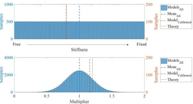
7.3 Single Model Analysis using Bayes Theorem ... 85
7.4 Multiple Model Analysis using Bayes Theorem ... 94
7.5 Conclusions ... 104
8. PHASE II: TEMPERATURE-DRIVEN ST-ID STUDY – CANTILEVER TRUSS BRIDGE ... 107
8.1 Field Experiment ... 108
8.2 Numerical Models ... 141
8.3 Single Model Analysis using Bayes Theorem ... 147
8.4 Multiple Model Analysis using Bayes Theorem ... 155
8.5 Conclusions ... 167
9. PHASE III: SYNTHESIS OF TEMPERATURE-DRIVEN BRIDGE STUDIES ... 171
9.1 Temperature-Driven Value ... 172
9.2 Investigation of Bridge Studies ... 173
10. PHASE IV: TEMPERATURE-DRIVEN FRAMEWORK AND GUIDANCE ... 192
10.1 Structure Details ... 194
10.2 Monitoring Criteria ... 198
10.3 Data and Analysis ... 199
11. CONCLUSIONS ... 209
12. RECOMMENDATIONS FOR FUTURE WORK ... 211
12.1 Continuation of Presented TD Evaluation Method ... 211
12.2 Thermal Evaluation through Artificial Neural Networks ... 218
13. SUMMARY ... 225
REFERENCES ... 227
APPENDIX A ADDITIONAL FIGURES OF SECTION 7 ... 241
LIST OF FIGURES
Page
Figure 1: Levels of Structural Health Monitoring (Rytter 1993) ... 4
Figure 2: Structural Identification Concept ... 5
Figure 3: Structural Identification Process (Reprinted from Catbas et al. 2013) ... 7
Figure 4: Field Testing Methods for Structural Monitoring ... 9
Figure 5: Temperature-Driven Concept (Reprinted from Murphy and Yarnold 2017) ... 14
Figure 6: Temperature-Driven Structural Identification Process (Reprinted from Murphy and Yarnold 2017) ... 18
Figure 7: Example of Partially Restrained W10x54 Beam Subjected to Uniform Thermal Loading (Reprinted from Murphy and Yarnold 2018) ... 20
Figure 8: Example Results for Varying Translational Stiffness Values of a W10x54 Steel Member (Modulus of Elasticity = 200 MPa, Coefficient of Thermal Expansion = 11.7x10⁻⁶ /℃, Cross-sectional Area = 10,200 mm2, and Length = 50 m): a) Unrestrained Displacement vs. Temperature and b) Restrained Strain vs. Temperature (Reprinted from Murphy and Yarnold 2018) ... 23
Figure 9: Thermal Gradient Effects from Direct Sunlight: a) Structure, b) Thermal Gradient, c) Deformed Shape, and d) Gradient Forces... 24
Figure 10: Thermal Gradient Effects from Precipitation: a) Structure, b) Thermal Gradient, c) Deformed Shape, and d) Gradient Forces... 25
Figure 11: Stress Distributions for Thermal Gradients: a) Structure, b) Temperature Gradient, c) Restrained Stress, d) Bending Stress, e) Axial Stress, and f) Total Stress ... 27
Figure 12: Sample Space of a Deterministic Approach ... 32
Figure 13: Sample Space of 500 Samples via Monte Carlo (MC) Simulations ... 33
Figure 14: Sample Space for 500 Samples via Latin Hypercube Sampling (LHS) ... 35
Figure 17: Sample Space for 50,000 Total Samples ... 46
Figure 18: Calibrated Model Parameters of the Spring Stiffness and CTES Multiplier ... 48
Figure 19: Calibrated Model Response of the Unrestrained Displacement and Restrained Strain ... 49
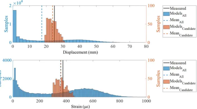
Figure 20: Candidate Model Response of the Unrestrained Displacement and Restrained Strain ... 51
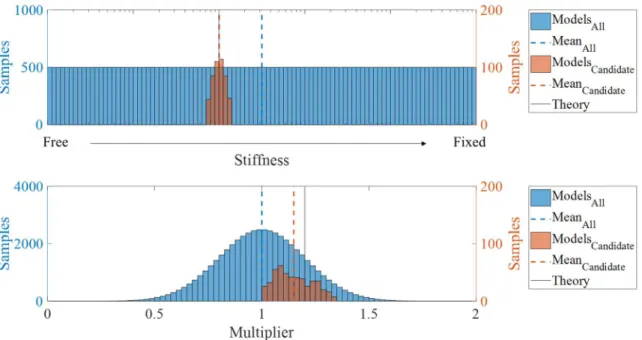
Figure 21: Candidate Model Parameters of the Spring Stiffness and CTES Multiplier ... 53
Figure 22: Overview of Research Approach: Phases of Completion ... 55
Figure 23: Route 61 Bridge: a) Structure, b) Location, and c) Orientation ... 59
Figure 24: Route 61 Overview (Reprinted from Murphy and Yarnold 2018) ... 60
Figure 25: Deck Cross-section ... 61
Figure 26: Evidence of Deterioration: a) Cracking along concrete sidewalk, b) Section loss at abutment, c) Spalling on barrier, d) Lateral displacement of barrier, e) Deformed guardrail support, and f) Extended neoprene bearing (Reprinted from Murphy and Yarnold 2018) ... 62
Figure 27: Finite Element Model of the Route 61 Bridge (Reprinted from Murphy and Yarnold 2018) ... 63
Figure 28: Sensitivity Study (Reprinted from Yarnold and Wilson 2015) ... 64
Figure 29: Instrumentation Plan (Reprinted from Murphy and Yarnold 2018) ... 65
Figure 30: Sensing Equipment: a) Strain Gage and b) Displacement Gage (Reprinted from Murphy and Yarnold 2018) ... 67
Figure 31: Data Acquisition Equipment: a) DAQ Setup and b) Solar Panel (Reprinted from Murphy and Yarnold 2018) ... 68
Figure 32: Installation Photos: a) Strain Gage on Interior Girder, b) Strain Gage on East Exterior Girder and c) Strain Gage on West Exterior Girder ... 69
Figure 33: Average Temperature Recorded from All Thermistors ... 70
Figure 35: Measured Microstrain for Web of Girder 2 at Abutment 2 ... 71
Figure 36: Measured Microstrain for Web of Girder 5 at Abutment 2 ... 71
Figure 37: Measured Microstrain for Bottom Flange of Girder 6 at Abutment 2 ... 72
Figure 38: Measured Microstrain for Web of Girder 2 at Pier 2 ... 72
Figure 39: Measured Microstrain for Web of Girder 5 at Pier 2 ... 72
Figure 40: Measured Displacement of Girder 5 at Abutment 2 ... 73
Figure 41: Measured Displacement of Girder 2 at Abutment 2 ... 73
Figure 42: Sunrise and Sunset Paths throughout Monitoring Period ... 74
Figure 43: Sunrise and Sunset Paths for Initialization Time on March 28, 2014 ... 75
Figure 44: Temperature Time Histories and Measured Responses for West Side of Bridge on March 30, 2014 ... 77
Figure 45: Temperature Time Histories and Measured Responses for East Side of Bridge on March 30, 2014 ... 78
Figure 46: Measured Strain Response of Bottom Flange of Exterior Girders at Abutment 2: a) Girder 1 and b) Girder 6 ... 80
Figure 47: Measured Strain Response of Web of Interior Girders at Abutment 2: a) Girder 2 and b) Girder 5 ... 80
Figure 48: Measured Strain Response of Web of Interior Girders at Pier 2: a) Girder 2 and b) Girder 5 ... 81
Figure 49: Displacement Response of Interior Girders at Abutment 2: a) Girder 2 and b) Girder 5 ... 81
Figure 50: Model Parameters ... 82
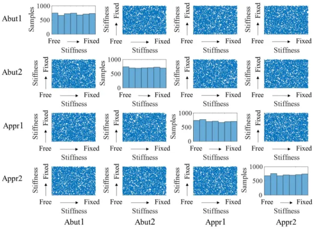
Figure 51: Sample Space for first 5,000 Samples of the 100,000 Total Samples ... 85
Figure 52: Calibrated Model Parameters of Abutments: a) Abutment 1 and b) Abutment 2 ... 87
Figure 53: Calibrated Model Parameters of Approaches: a) Approach 1 and b) Approach 2 ... 88 Figure 54: Calibrated Model Strain Response of Bottom Flange of Exterior
Figure 55: Calibrated Model Strain Response of Web of Interior Girders at
Abutment 2: a) Girder 2 and b) Girder 5 ... 91
Figure 56: Calibrated Model Strain Response of Web of Interior Girders at Pier 2: a) Girder 2 and b) Girder 5 ... 92
Figure 57: Calibrated Model Displacement Response of Interior Girders at Abutment 2: a) Girder 2 and b) Girder 5 ... 93
Figure 58: Candidate Model Strain Response of Bottom Flange of Exterior Girders at Abutment 2: a) Girder 1 and b) Girder 6 ... 95
Figure 59: Model Strain Response of Web of Interior Girders at Abutment 2: a) Girder 2 and b) Girder 5 ... 96
Figure 60: Model Strain Response of Web of Interior Girders at Pier 2: a) Girder 2 and b) Girder 5 ... 97
Figure 61: Model Displacement Response of Interior Girders at Abutment 2: a) Girder 2 and b) Girder 5 ... 98
Figure 62: Refined Model Parameters of Abutments: a) Abutment 1 and b) Abutment 2 ... 100
Figure 63: Refined Model Parameters of Approaches: a) Approach 1 and b) Approach 2 ... 101
Figure 64: Thermal Evaluation Results: a) Original, b) Current, and c) Recommended (Reprinted from Murphy and Yarnold 2018) ... 102
Figure 65: Hurricane Bridge: (a) Structure, (b) Location, and (c) Orientation ... 109
Figure 66: Hurricane Bridge Overview ... 110
Figure 67: Cantilevered and Suspended Section Configuration ... 111
Figure 68: Pin and Hanger Assembly ... 112
Figure 69: Boundary Conditions: a) Piers 3 and 7, b) Piers 4 and 6, and c) Pier 5 ... 113
Figure 70: Auxiliary Support System (Catch System) ... 114
Figure 71: Retrofitted Truss Members ... 114
Figure 72: Deck Width Dimensions: a) Original Design and b) Rehabilitated Design ... 115
Figure 73: Finite Element Model of the Hurricane Bridge (Reprinted from
Murphy and Yarnold 2017) ... 116 Figure 74: Sensitivity Study of Bottom Chord Strain (Reprinted from Murphy
and Yarnold 2017) ... 118 Figure 75: Instrumentation Locations Resulting from the Sensitivity Study
(Reprinted from Murphy and Yarnold 2017) ... 119 Figure 76: Final Instrumentation Plan (Reprinted from Murphy and Yarnold
2017) ... 120 Figure 77: Gages: a) 152-Millimeter (6-Inch) Strain Gage and b) Displacement
Gage ... 122 Figure 78: Data Acquisition Equipment: a) Solar Panel, b) DAQ Box, and c)
Ground Station Box (Reprinted from Murphy and Yarnold 2017) ... 123 Figure 79: Installation Photos: a) Gage Cable Securement and Installation of
Strain Gage on Vertical Member, b) Strain Gage Installation on Catch System, c) Cable Assistance from Bridge Deck, and d) Displacement
Gage Installation ... 124 Figure 80: Average Ambient Temperature Measured from Displacement Gages ... 125 Figure 81: Measured Displacement for Pier 5: a) Deck Level and b) Bearing
Level ... 126 Figure 82: Measured Displacement for Pier 7: a) Deck Level and b) Bearing
Level ... 127 Figure 83: Sunrise and Sunset Paths throughout Year ... 128 Figure 84: Sunrise and Sunset Paths for Initializing Data Point on March 18,
2017 ... 129 Figure 85: Temperature Time History and Measured Displacement Response on
April 13, 2017 ... 131 Figure 86: Measured Displacement Response: a) Pier 5 Deck Level, b) Pier 7
Deck Level, c) Pier 5 Bearing Level, and d) Pier 7 Bearing Level ... 133 Figure 87: Global and Local Out-of-Plane Bending of Upper Chord Members at
Pier 7 ... 134 Figure 88: Strains from Diagonal at Pier 7 ... 135
Figure 89: Behavior at Upper Chord of Pier 5: a) Strain vs. Temperature, b) Displacement vs. Temperature, c) Displacement vs. Strain,
d) All Responses-View 1, and e) All Responses-View 2 ... 137
Figure 90: Behavior at Lower Chord of Pier 5: a) Strain vs. Temperature, b) Displacement vs. Temperature, c) Displacement vs. Strain, d) All Responses-View 1, and e) All Responses-View 2 ... 138
Figure 91: Behavior at Upper Chord of Pier 7: a) Strain vs. Temperature, b) Displacement vs. Temperature, c) Displacement vs. Strain, d) All Responses-View 1, and e) All Responses-View 2 ... 139
Figure 92: Behavior at Lower Chord of Pier 7: a) Strain vs. Temperature, b) Displacement vs. Temperature, c) Displacement vs. Strain, d) All Responses-View 1, and e) All Responses-View 2 ... 140
Figure 93: Sample Space for first 2,000 of 100,000 Total Samples ... 146
Figure 94: Calibrated Model Parameters of Pier 7: a) Deck and b) Bearing ... 148
Figure 95: Calibrated Model Parameters of Pin and Hanger: a) Top and b) Bottom ... 149
Figure 96: Calibrated Model Parameters of Pier 5: a) Deck and b) Bearing ... 150
Figure 97: Calibrated Model Parameter of Pier 6 ... 150
Figure 98: Calibrated Model Parameters of Modulus of Elasticity: a) Steel and b) Concrete ... 151
Figure 99: Calibrated Model Parameters of Coefficient of Thermal Expansion: a) Steel and b) Concrete ... 152
Figure 100: Calibrated Model Displacement Response of Pier 5: a) Top and b) Bottom ... 154
Figure 101: Calibrated Model Displacement Response of Pier 7: a) Top and b) Bottom ... 154
Figure 102: Model Displacement Response of Pier 5: a) Top and b) Bottom ... 156
Figure 103: Model Displacement Response of Pier 7: a) Top and b) Bottom ... 156
Figure 104: Refined Model Parameters of Pier 7: a) Deck and b) Bearing ... 158
Figure 105: Refined Model Parameters of Pin and Hanger: a) Top and b) Bottom ... 159
Figure 106: Refined Model Parameters of Pier 5: a) Deck and b) Bearing ... 160
Figure 107: Refined Model Parameter of Pier 6 ... 160
Figure 108: Refined Model Parameters of Modulus of Elasticity: a) Steel and b) Concrete ... 161
Figure 109: Refined Model Parameters of Coefficient of Thermal Expansion: a) Steel and b) Concrete ... 162
Figure 110: Tacony-Palmyra Bridge (Reprinted from Yarnold et al. 2012b) ... 175
Figure 111: Streicker Bridge (Courtesy of Google Maps) ... 176
Figure 112: Ricciolo Vedeggio Viaduct (Reprinted from Glisic et al. 2008) ... 178
Figure 113: Dashengguan Yangtze River Bridge (Reprinted from Ding et al. 2015) ... 179
Figure 114: Hernando Desoto Bridge (Courtesy of Google Maps) ... 180
Figure 115: I-35W St. Anthony Falls Bridge (Courtesy of Google Maps) ... 181
Figure 116: Commodore Barry Bridge (Courtesy of Google Maps) ... 182
Figure 117: Cleddau Bridge (Reprinted from Kromanis and Kripakaran 2014) ... 184
Figure 118: Zhanjiang Bay Bridge (Courtesy of Google Maps) ... 185
Figure 119: Jiangyin Yangtze River Bridge (Courtesy of Google Maps) ... 186
Figure 120: Jiubao Bridge (Reprinted from Zhou et al. 2017) ... 187
Figure 121: Tsing Ma Bridge (Courtesy of Google Maps) ... 188
Figure 122: Tamar Bridge (Reprinted from Jesus et al. 2018) ... 189
Figure 123: Humber Bridge (Courtesy of Google Maps) ... 190
Figure 124: Example of TD Framework using Parameters from only TS #1 and TS#2 ... 193
Figure 125: Temperature-Driven Performance Evaluation Guidance ... 208
Figure 126: Thermal Gradients: a) Structure, b) Transverse Gradient, c) Longitudinal Gradient, d) Vertical Gradient, and e) Combined Gradient ... 212
Figure 127: Thermal Gradient Distributions: a) Single Gradient through Entire section, b) Single Gradient through Portion of the
Cross-section, and c) Double Gradient through Portion of Cross-section ... 213
Figure 128: Process for Model Parameter Comparisons using Structural Models with Thermal Gradients ... 215
Figure 129: Damage Scenarios and Indices ... 216
Figure 130: Candidate Model Data: a Model Parameter and b) Damage Index ... 218
Figure 131: Artificial Neural Network Concept for Thermal Evaluation ... 220
Figure 132: Temperature Field and Measured Responses for the Route 61 Bridge ... 221
Figure 133: Perceptrons of the ANN: a) Single and b) Multiclass ... 222
Figure 134: Response Prediction using Trained Data ... 223
Figure 135: Damage Identification using ANNs of Simulated Data ... 224
Figure 136: Measured Strain Response of Bottom Flange of Exterior Girders at Abutment 2 on March 30, 2014: a) Girder 1 and b) Girder 6 ... 242
Figure 137: Measured Strain Response of Web of Interior Girders at Abutment 2 on March 30, 2014: a) Girder 2 and b) Girder 5 ... 242
Figure 138: Measured Strain Response of Web of Interior Girders at Pier 2 on March 30, 2014: a) Girder 2 and b) Girder 5 ... 243
Figure 139: Measured Displacement Response of Interior Girders at Abutment 2 on March 30, 2014: a) Girder 2 and b) Girder 5 ... 243
Figure 140: Measured Displacement Response on April 7, 2017: a) Pier 5 Deck Level, b) Pier 7 Deck Level, c) Pier 5 Bearing Level, and d) Pier 7 Bearing Level ... 245
LIST OF TABLES
Page Table 1: Calibrated Model Percent Difference with Respect to Theoretical
Parameter Values ... 48
Table 2: Calibrated Model Percent Difference with Respect to Measured Responses ... 50
Table 3: Candidate Model Response Distributions ... 52
Table 4: Candidate Model Parameter Distributions ... 54
Table 5: Research Schedule: Phases of Completion ... 57
Table 6: Calibrated Model Parameters ... 88
Table 7: Calibrated Model Responses ... 93
Table 8: Candidate Model Response Distributions ... 99
Table 9: Candidate Model Parameter Distributions ... 102
Table 10: Prior Probability Distributions of Boundary/Continuity Parameters ... 144
Table 11: Prior Probability Distributions of Material Property Parameters ... 145
Table 12: Calibrated Model Parameters ... 153
Table 13: Calibrated Model Response ... 155
Table 14: Candidate Model Response Distributions ... 157
Table 15: Boundary/Continuity Model Parameter Distributions ... 163
Table 16: Material Property Model Parameter Distributions ... 163
Table 17: Response Distributions with Pier 7 Deck excluded from Calibration ... 164
Table 18: Response Distributions with Pier 7 Bearing excluded from Calibration ... 165
Table 19: Response Distributions with Pier 5 Deck excluded from Calibration ... 166
Table 20: Response Distributions with Pier 5 Bearing excluded from Calibration ... 167
Table 22: Guidance for TD Evaluations... 194 Table 23: TS Framework: Project Details ... 202
1. INTRODUCTION AND MOTIVATION
In the United States, the average bridge is approximately 43 years old with nearly 4 out of every 10 bridges currently 50 years or older (ASCE 2017). Many of these structures are reaching their design lives at the same time. As a result, a significant number of bridges are in need of intervention. Not only is aging infrastructure a concern, but newer structures may also need repair due to structural deficiency. These problems may be due to instances such as overloading, poor maintenance, or inadequate design to name a few. Due to the large volume of bridges in need of repair and limited financial resources, engineering practices have migrated to more rehabilitative approaches rather than complete replacements. This mentality allows engineers to stagger the scheduling of major bridge replacements rather than attempt them simultaneously. With nearly 58,495 bridges in the United States deemed structurally deficient and in need of intervention, prioritization has become necessary to determine the order in which bridges are rehabilitated or replaced (ARTBA 2016). One way of doing this is through structural monitoring. Contractors, engineers, researchers, and bridge inspectors acknowledge structural monitoring is beneficial but needs improving (Figueiredo et al. 2013). The structural monitoring research presented herein intends to advance the knowledge of a novel, temperature-driven approach to structural monitoring and develop a framework to assist engineers/researchers when using this process to evaluate bridge performance.
2. OBJECTIVES
The primary objectives of this research are to advance the knowledge of a temperature-driven structural evaluation technique and create a framework to assist engineers/researchers when using this method to evaluate bridges. Guidelines regarding the applicability and limitations of this method are investigated and developed by utilizing two unique bridge studies conducted by the author and a synthesis of similar studies from various researchers and practicing engineers. These projects encompass a wide variety of parameters that contribute to the knowledge and guidance of using temperature to assess the structural integrity of bridges. In particular, this research aims to address the following objectives with respect to the bridge geometry, bridge composition, movement systems, and monitoring criteria:
Temperature-Driven Value: Determine if this evaluation technique can provide valuable information pertaining to the structural health or behavior of a bridge. Explore any successes and failures of using the temperature-driven method.
Temperature-Driven Framework: Investigate how temperature-driven evaluations are performed and the project logistics utilized by each study.
3. BACKGROUND AND LITERATURE REVIEW
Bridge monitoring encompasses a wide range of procedures and methodologies, the most common of which are visual inspections and field testing. As common practice, bridges often undergo visual inspections by appropriately trained personnel. These inspections typically reveal any obvious degradation (e.g. cracks or rust on a steel girder) that may affect the integrity of the structure. Although visual inspections are beneficial, investigations from the Federal Highway Administration (FHWA) have revealed a significant lack of reliability from these field inspections alone (FHWA 2001). A more efficient and comprehensive method of evaluating bridge behavior is possible via field testing (Aktan et al. 1997; Bakht and Jaeger 1990; Catbas and Aktan 2002).
Structural monitoring through field testing is a means of evaluating a structure based on its performance rather than age or appearance. This monitoring technique allows for engineers, consultants, and owners to possess information regarding modal or numerical characteristics to validate a bridge’s structural integrity. Field testing has been shown to identify numerical characteristics such as strains, displacements, and rotations as well as modal characteristics such as mode shapes and frequencies (Karbhari and Lee 2009). These characteristics can provide a more comprehensive evaluation when investigating deterioration such as fatigue cracks and condition assessment of bridge decks (Chong et al. 2003). The path from field testing to evaluation of a structure can be an extensive and complex process; therefore, guides for evaluating constructed systems have been developed. Two common processes are known as Structural Health Monitoring (SHM) and Structural
3.1 Structural Health Monitoring (SHM)
SHM is the process of utilizing continuous, global observation and analysis of a structure to extract information about its current state of health (Farrar and Worden 2007). SHM systems vary in robustness according to specific objectives of individual projects. Shown in Figure 1, the basic framework for SHM is typically defined in levels, each encompassing the extent of the level prior and increasing the robustness of the monitoring system (Rytter 1993). SHM systems use sensor technology to track the structural behavior and identify any changes over time. These systems are used to quantify bridge behavior in order to efficiently manage bridges with regard to degradation, obsolescence, maintenance, and security (Alampalli et al. 2005; Alampalli and Ettouney 2008; Del Grosso 2013). Many SHM systems include real-time monitoring with alert notifications to quickly inform engineers and bridge owners of significant changes (Masri et al. 2004; Yarnold et al. 2012b).
Figure 1: Levels of Structural Health Monitoring (Rytter 1993) Level 4: Prediction
Level 3: Assessment Level 2: Localization Level 1: Detection
• Evaluate impact of damage. • Estimate remaining useful life. • Estimate severity of damage.
• Determine the location of damage.
3.2 Structural Identification (St-Id)
St-Id is the process of using sensing technology and structural modeling to assess the performance of a constructed system within a specified time period (Catbas et al. 2013). Liu and Yao originally developed the theory behind St-Id for civil-structural engineering purposes in 1978 (Liu and Yao 1978). The primary goal of St-Id is to identify a structural model or models that accurately represent the behavior of a structure. These models are then used to provide insight regarding the health and performance of the structure. The overall concept of St-Id is shown in Figure 2 below.
St-Id utilizes two unique components: the physical structure and numerical models. With regard to the physical structure, measured responses are collected by means of conducting a field experiment. A monitoring system is installed on the structure and records the structure’s response as it is subjected to a load. As a result, these measured responses provide a quantitative representation of the structure’s behavior. Pertaining to the numerical models, a collection of structural models is usually developed via finite element analyses. Model parameters corresponding to specific conditions of the structure are varied to develop a sample space. The sample space is a collection of parameter combinations that are individually subjected to a finite element analysis and produce structural models that encapsulate many different behaviors of the structure. The measured responses are then compared to corresponding responses of the structural models within the structural identification analysis with either a single model or multiple model approach.
In 2005 Aktan and Moon shaped the structural identification concept into a comprehensive framework for evaluating constructed systems using a single model approach (Aktan and Moon 2005). Moon later evolved the process into a multiple model approach as well (Beck and Katafygiotis 1998; Goulet et al. 2010; Moon 2008; Ravindran et al. 2007; Smith and Saitta 2008). Both approaches are outlined in depth in the following sections. 3.2.1 Single Model Structural Identification (SM St-Id)
The single model (SM) St-Id process shown in Figure 3 was developed by Aktan and Moon and is a six step procedure for evaluating constructed systems. With this technique, only one structural model is identified to represent the behavior of the structure. Each step of the process is thoroughly outlined in Catbas et al. (2013) and condensed in the sections below.
Figure 3: Structural Identification Process (Reprinted from Catbas et al. 2013)
3.2.1.1Step 1: Observation and Conceptualization
The initial step of SM St-Id is “Observation and Conceptualization” during which an understanding of the structure and motivation of the investigation is developed. In many cases, the presence of damage provokes an inquiry as to why the damage exists or how quickly the damage is progressing. Another common motivation is simply the lack of confidence and information about a structure’s integrity. For example, the structural behavior of aged bridges or those with extensive retrofits may be more complex and different than the original design. Thus, an assessment may be necessary to understand the structural behavior of such bridges. During this step, all available pertinent information about the structure and its behavior is gathered. This includes but is not limited to original drawings, rehabilitation drawings, inspection reports, and site visits to name a few. In-depth
and for proper modeling in Step 2. With all of the structure information available, conceptualization of the project begins by identifying specific objectives as well as potential challenges.
3.2.1.2Step 2: A-Priori Modeling
With many model types used to evaluate structures, analytical models are generally classified into two categories: non-physics-based and physics-based. Non-physics-based models are primarily data-driven and utilize a variety of numerical techniques such as probabilistic or statistical approaches (Catbas et al. 2013). However, physics-based models most commonly utilize geometric approaches such as finite element or modal models. Physics-based models are specifically designed to address behavior parameters such as equilibrium, movement mechanisms, continuity, and boundary conditions (Catbas et al. 2013). For this reason, St-Id primarily applies to physics-based models. “A-priori Modeling” consists of creating a physics-based model that represents the as-designed or theoretical behavior of the structure. Depending on the structure and the objectives of the assessment, the a-priori model can range from a low resolution phenomenological model to a high resolution finite element model. The purposes of the a-priori model are to establish a baseline of how the structure in question is designed to behave and to determine sensitive areas of the structure that are most beneficial for monitoring. Based on those areas, the monitoring system is designed and implemented during the third step, “Controlled Experiment”.
3.2.1.3Step 3: Controlled Experiment
The next step of the SM St-Id process is “Controlled Experiment”, wherein the monitoring system is designed/installed and field testing is conducted. While designing the
controlled experiment, logistics of the bridge itself such as access, closure availability, and project budget are taken into consideration. These restrictions potentially influence the type or robustness of the monitoring system being designed. The monitoring system logistics such as monitoring duration, monitoring/data acquisition equipment, sensor type/resolution, sampling rate, and power requirements are generally dependent on the type of field testing being conducted. Controlled experiment techniques include field testing with respect to static loads, vibrations, and temperature (Figure 4).
Figure 4: Field Testing Methods for Structural Monitoring Field Testing Static Load Input/Output Relationship Measurable stationary load excites the bridge
(vehicle, weight, etc.) Vibration Ambient Output-Only Relationship Non-measurable ambient conditions excite the bridge (wind, traffic loads, etc.) Dynamic Input/Output Relationship Measurable applied forcing function excites the bridge (live loading, shaker, impact device, etc.) Temperature Input/Output Relationship Measurable ambient condition
excites the bridge (temperature)
3.2.1.3.1 Static Load Testing
Static load testing is an input-output field testing procedure in which the input is a stationary or low-speed load and the output is the structure’s response to the load. Often, static load tests on bridges use inputs like weights or vehicles (trucks or railcars) with known measurements of force applied from each axle. Static load tests in which the load is completely stationary are referred to as park tests. During a park test, a vehicle is driven to a predetermined location on the bridge and parked, remaining completely stationary until measurements are recorded. Once the measurements are recorded, the vehicle moves to another position to record additional measurements. The vehicle is parked at various locations on the bridge until sufficient amounts of data are collected. Live load static testing is the process of using a vehicular load moving at a low-speed to excite a bridge. This method of testing is known as a crawl test. During a crawl test, the load (vehicle) travels along the bridge at a low speed while measurements are recorded. Although the vehicle is non-stationary, the bridge does not experience dynamics effects due to the low-speed travel. Crawl tests are used to divulge various types of information including the composite action of decks and girders, neutral axis location, live load distribution factors, span continuity, load ratings, and load carrying capacity (Bakht and Jaeger 1990; Barr et al. 2001; Bell et al. 2013; Breña et al. 2013; Chajes and Shenton 2006; Eom and Nowak 2001; James 2016; James and Yarnold 2017). Other outputs of static testing include a variety of responses including girder deflections / rotations and flexural strains or even cable forces on a cable-stayed bridge (Bacinskas et al. 2013; Fang et al. 2004).
3.2.1.3.2 Vibration Testing 3.2.1.3.2.1 Ambient
Currently, the most prevailing technique for monitoring long-span bridges is ambient vibration monitoring. This technique monitors a structure under ambient loading conditions such as vehicular or pedestrian traffic, wind, ocean waves, or low-intensity seismic loads (Abdel-Ghaffar and Scalan 1985; Coppolino and Rubin 1980; Farrar et al. 1999; Nakamura and Sakamoto 2000). Using this method, modal parameters such as natural frequencies, mode shapes, and damping can be determined and tracked for a structure (Bolton et al. 2001; Karbhari and Lee 2009; Kim et al. 2005; Mazurek and Dewolf 1990). With this information, the location and extent of damage can be identified and assessed (Bolton et al. 2005; Kim and Stubbs 1995; Park et al. 2002). Although this method has been utilized, ambient vibration monitoring also has challenges associated with it (Catbas et al. 2007; Karbhari and Lee 2009). Ambient vibration monitoring is limited to low frequency excitation (Karbhari and Lee 2009). This method also has difficulty dealing with measurable inputs and environmental effects. These effects can be of the same order of magnitude as damage effects, making identification of damage difficult to achieve (Peeters and De Roeck 2001; Sohn 2007). Although removing temperature effects is possible (Zhu et al. 2016), these effects still pose a significant challenge for this type of testing. The prevailing reason for the limited success of ambient vibration monitoring of long-span bridges is the limited sensitivity to structural damage (Brownjohn et al. 2011).
3.2.1.3.2.2 Dynamic
utilizes a measurable input-output relationship to assess the structural integrity of a bridge. Dynamic displacements and modal properties such as natural frequencies, mode shapes, and damping ratios can be determined (Bacinskas et al. 2013). Live load dynamic testing can also provide insight on load distribution throughout the bridge (Eom and Nowak 2001) as well as composite action between the superstructure and the deck (Alampalli and Kunin 2003). This method is generally the most common technique to assess relatively small structures due to their heightened sensitivity to live loads. However, large-scale structures often have a low sensitivity to live loading. This along with temperature challenges similar to ambient vibration testing can increase the difficulty of identifying effects from live load testing. Structural excitation is also achievable through the use of impact (i.e. dropping a weight or using an impact hammer) or shakers (Farrar et al. 1999).
3.2.1.3.3 Temperature Testing
Temperature effects from daily or seasonal temperature changes are often significant enough to warrant consideration regardless of the type of test being performed (Catbas et al. 2007; Del Grosso and Lanata 2014; De Roeck 2003). Temperature effects are often filtered out of analysis processes or accounted for during field testing procedures. For example, while static load testing a cable-stayed bridge in Taiwan, researchers removed the static load from the bridge every two hours to reinitialize the data and mitigate temperature effects (Fang et al. 2004). However, in recent years, temperature has been used to excite structures for damage detection and performance evaluation (Cao et al. 2010; Glisic et al. 2008; Kulprapha and Warnitchai 2012; Yarnold et al. 2012a; Zhou et al. 2018). Since bridges have a high sensitivity to thermal effects, everyday temperature exposure can excite a response from the structure. The temperature-driven concept utilizes this cause-and-effect
relationship to develop a behavioral signature for the bridge. This process is detailed in Figure 5 below. The temperature variations (input) are quantifiable and can be measured simultaneously with the member strains, displacements, and/or rotations (output) that the bridge experiences in response to the thermal load. This input-output relationship can be used to identify and monitor unknown quantifiable information with regard to the bridge (e.g. boundary conditions, continuity conditions, force distribution, etc.). Once the behavioral signature has been determined, it can be used to update a model and represent the current condition of the structure.
Figure 5: Temperature-Driven Concept (Reprinted from Murphy and Yarnold 2017)
3.2.1.4Step 4: Processing and Interpretation of Data
Next, in “Processing and Interpretation of Data”, data is collected from the monitoring system and quality checked. Any erroneous data (possibly from malfunctioning sensors or electrical interference, for example) is identified and subsequently removed from analysis. Also, investigation of specific information through windowing, filtering, or averaging is possible during this step. If appropriate, direct data interpretation is performed.
Since the data is available, non-physics-based numerical models such as artificial neural networks and auto-regressive models are also used to analyze and process data. Any conclusions based solely on the data are determined.
3.2.1.5Step 5: Model Calibration and Parameter Identification
In Step 5 “Model Calibration and Parameter Identification”, variable parameters such as boundary or continuity conditions are identified for the calibration process. Using optimization algorithms such as objective functions or maximum likelihood estimations (further discussed later in Section 5), the preliminary model developed in Step 2 is calibrated with the measured results from Step 4 to identify a single model that depicts the structure and its behavior in its current condition. Parameters from the calibrated model are used to identify conditions of the structure.
3.2.1.6Step 6: Utilization of Model for Simulations
Finally, in Step 6 the calibrated model is used for simulations and to acquire more knowledge about the structure in its current state. This model is also used to predict responses of the structure. With the information acquired from the calibrated model, engineers are able to conduct a proper assessment of the structure’s behavior and integrity. The calibrated model is intended to assist engineers and owners with decisions regarding maintenance, rehabilitation, or potential retrofit.
3.2.2 Multiple Model Structural Identification (MM St-Id)
The multiple model (MM) St-Id technique described within Moon (2008) is beneficial when many different structural models, each with varying parameter combinations, are capable of reasonably describing the structural behavior (also referred to
as nonuniqueness). The multiple model approach evolves from the single model approach by modifying Steps 5 and 6 to consider more than one calibrated model.
3.2.2.1Step 5 Modification: Model Calibration and Parameter Identification
Engineering experience, data mining, or calibration techniques reduce the large number of structural models to a predetermined number of most probable scenarios called candidate models. Distributions of the model parameters and predictive responses are used to reduce uncertainty of the behavior and conditions of the structure.
3.2.2.2Step 6 Modification: Utilization of Models to Identify Trends
Rather than using each of the candidate models individually, the information from all of the candidate models is used collectively to identify trends. Distributions of the responses are used to better understand the behavior of the structure.
Both the single and multiple model approaches have the potential to assist engineers and bridge owners with decisions regarding a structure’s health and maintenance; however, in some cases, one method may prove superior over the other. One major benefit of the single model approach is that direct information is provided by utilizing just one model. For instance, if the model was developed within a finite element software, an engineer could open the model file and have all the capabilities and amenities of the finite element software available to analyze the structure. Unfortunately, this commodity does not extend to the multiple model approach. Since a number of models influence the definition of the behavior of the bridge, an engineer cannot simply open and analyze all of the models simultaneously. The multiple modeling approach can, however, provide information about the importance or sensitivity of a parameter to the load scenario. For example, within a set of candidate models one parameter may converge to a discrete value (indicating a heightened sensitivity) whereas
another may vary significantly (indicating a reduced sensitivity). An engineer may then be able to identify which parameters have more influence over the behavior of the structure.
The St-Id process has been successful in laboratory/small scale settings (Jesus et al. 2016, 2017; Mazurek and Dewolf 1990). However, one of the primary disadvantages of St-Id is the difficulty of experimenting on an actual structure (Aktan et al. 1997; Catbas and Aktan 2002). In reality, structures are often complex and difficult to model accurately which is crucial for model-based evaluation (Yuen et al. 2004). In addition, the logistics of conducting an experiment on a large structure are substantial. Researchers are often forced to make assumptions for experiment variables out of their control, introducing more possibility for errors. Often structures must be monitored for long periods of time before a reliable evaluation of the structure can be completed (Sikorsky et al. 2001). For the purpose of this research, a temperature-driven approach to the St-Id process is currently being explored.
3.3 Temperature-Driven Structural Identification (TD St-Id)
The temperature-driven (TD) approach to the St-Id process (Figure 6), where thermal “loads” are treated as the excitation and the corresponding static responses are correlated, shows promise to mitigate many of the shortcomings of ambient vibration monitoring (Kromanis and Kripakaran 2016; Yarnold and Moon 2015). Logistically, TD St-Id can be performed continuously over a period of time with minimal data storage and time synchronization requirements. In addition, the equipment is relatively inexpensive and generally self-sustaining with little need for man-power resources once the system is installed and operational. The results can be recorded throughout the structure’s changing
wind, ice, impact, or similar nature. This is primarily due to the fact that a TD baseline is highly sensitive to many changes of structural systems (Laory et al. 2013; Yarnold and Moon 2015). TD monitoring is particularly useful for large structures. Long-span bridges, for example, are more responsive to thermal loads than live loads, making the results easier to identify.
Figure 6: Temperature-Driven Structural Identification Process (Reprinted from Murphy and Yarnold 2017)
4. CONCEPT
4.1 Thermal Behavior
In order to complete a TD structural analysis of a bridge, an extensive knowledge of thermal behavior is required. An insight into some of this knowledge is provided below. Construction material properties, structure geometry, and restraints imparted by boundary conditions heavily influence deflections, stresses, and strains that occur as results of thermal “loads”. Like most materials, bridge materials such as steel, concrete, and asphalt expand and contract in response to such loading. The physical make-up of these materials allows for unique rates of heating/cooling (quantified as thermal inertia) as well as expansion/contraction (quantified as coefficient of expansion) for each material. The coefficient of thermal expansion (α) directly relates how much the material expands or contracts, thus it affects the stress or strain in particular members of the bridge. Boundary conditions also affect the strain or stress in those members of the bridge. Boundary conditions can vary in extent of impeded motion; therefore, it is possible to have boundary conditions that are unrestrained, partially restrained, or fully restrained. If the structure is assembled in such a way that prevents movement from thermal effects, stress accumulates within the members.
4.2 Types of Thermal Loading
Another important aspect of thermal behavior is the type of thermal loading that the structure is experiencing. If the structure is subjected to a consistent temperature change throughout, the structure is experiencing uniform thermal loading. However, if the structure
warmer than others, the structure is experiencing thermal gradients. Each of these loading types is discussed further below.
4.2.1 Uniform Thermal Loading
To fully understand uniform thermal loading, Figure 7 provides an illustrative example of a partially restrained W10x54 beam, subjected to a uniform temperature change increase (ΔT). The structure is simply-supported and uses a spring to define the extent of restraint at one end of the member.
Figure 7: Example of Partially Restrained W10x54 Beam Subjected to Uniform Thermal Loading (Reprinted from Murphy and Yarnold 2018)
A critical aspect of thermal behavior is that the response includes an unrestrained portion and a restrained portion. Furthermore, the total displacement (δT) is a combination
of the unrestrained displacement (δU) and the restrained displacement (δR) and is calculated
according to Equation 1.
𝜹𝑻= 𝜹𝑼+ 𝜹𝑹 = 𝜶 𝚫𝑻 𝑳 (1)
The restrained displacement (δR) is the portion that produces stress in the member
(δU produces no stress). This restraint occurs as a result of the spring support exerting a
Equation 2, where A represents the cross-section area and E represents the modulus of elasticity.
𝜹𝑹 =𝑷𝑳
𝑨𝑬 (2)
The axial stress in the beam is simply the longitudinal axial force (P) divided by the cross-section area (A). Therefore, δR can also be expressed in terms of stress as shown in
Equation 3.
𝜹𝑹 = 𝝈 𝑳
𝑬 (3)
The unrestrained displacement (δU) can be calculated from the spring force (P) and
the stiffness of the spring (KS) as shown in Equation 4. 𝜹𝑼 = 𝑷
𝑲𝒔 (4)
Equations 1 through 4 show the total displacement and the unrestrained and restrained components of displacement due to thermal loading. Thermal strain can be determined in a similar fashion. As with displacement, strain induced from thermal loading is comprised of unrestrained and restrained components that can be calculated as well. This is achieved simply by dividing each of the prior displacement equations by the length (L).
As mentioned previously, the structure can have various levels of restraint. The partially restrained scenario is most prevalent in reality as unintended stiffness from weathering and exposure, for example, can affect the boundary conditions of the structural system. Since conditions may change naturally over time, the unintended stiffness of each boundary condition is generally unknown. Fortunately, the boundary conditions can be
determined using thermal strains and displacements since they are sufficiently sensitive to these parameters. Figure 8 shows how temperature change and boundary stiffness affect strains and displacement in the example described above. If the boundary stiffness was low in magnitude (1 kN/m, for example), a relatively large unrestrained displacement of nearly 30 mm for a 50℃ temperature change would be expected (Figure 8(a)). However, if the boundary stiffness was high or rigid, large measurements of nearly 600 microstrain of restrained strain would be expected (Figure 8 (b)). This simple uniform thermal load TD example illustrates how the input (temperature) and outputs (restrained strains and unrestrained displacements) can be used to identify a boundary condition (stiffness).
Figure 8: Example Results for Varying Translational Stiffness Values of a W10x54 Steel Member (Modulus of Elasticity = 200 MPa, Coefficient of Thermal Expansion =
11.7x10⁻⁶ /℃, Cross-sectional Area = 10,200 mm2, and Length = 50 m): a) Unrestrained Displacement vs. Temperature and b) Restrained Strain vs.
4.2.2 Thermal Gradients
Structures can also be affected by thermal gradients which occur when the thermal load applied to the structure is not uniform throughout. For example, thermal gradient effects can occur as the result of direct sunlight on a structure as shown in Figure 9. The parts of the bridge that are exposed to direct sunlight experience greater temperatures than those that are shielded from the direct radiation (Figure 9(b)). The structure reacts according to the temperature load experienced and thus can cause the overall structural behavior to be inconsistent. The side of the bridge with direct sunlight wants to expand like the unrestrained deformed shape shown in Figure 9(c). However, the assembly of the structure provides restraint and does not allow for such deformation. As a result, gradient forces occur. The warmer members of the bridge experience a compressive force since they want to expand but are unable. Conversely, the cooler members experience a tensile force since they want to contract but are unable.
Figure 9: Thermal Gradient Effects from Direct Sunlight: a) Structure, b) Thermal Gradient, c) Deformed Shape, and d) Gradient Forces
Thermal effects can also be present with other environmental conditions such as when precipitation collects on a structure as shown in Figure 10. When this happens, the precipitation causes the deck of the bridge to be cooler than the bridge structure beneath (Figure 10(b)). The deck contracts and the structure wants to bend upward (Figure 10(c)). However, restraint again causes gradient forces to occur. Tension occurs at the cooler surface, whereas compression occurs at the warm members underneath.
Figure 10: Thermal Gradient Effects from Precipitation: a) Structure, b) Thermal Gradient, c) Deformed Shape, and d) Gradient Forces
Thermal gradients are addressed by analyzing the stress distributions that occur as the temperature changes throughout a structure. The total stress from temperature gradients is comprised of restrained and unrestrained components. The restrained component, σrestrained, is calculated by rearranging Equation 1 to solve for the stress. The unrestrained
components can be determined by discretizing the structure into elements affected by thermal gradients. The unrestrained components are comprised of the bending and axial behavior caused by the differential temperature along the element. The differential temperature for each element can be determined by Equation 5, where 𝑇 is the temperature
of the element, y is the distance from the neutral axis, and 𝑦 is the distance to the element’s elastic centroidal axis from the neutral axis of the structure.
𝑻(𝒚) = 𝑻𝒂𝒊+∆𝑻𝒊
𝒅𝒊 (𝒚 − 𝒚𝒊) (5)
Then Equations 9 and 13 below can be used to calculate the stresses. To calculate the axial stresses, the axial strain must be determined using Equation 6, where α is the coefficient of thermal expansion of the material and A is the cross-sectional area of the structure.
𝜺 =𝜶
𝑨∫ 𝑻(𝒚) 𝒅𝑨 (6)
Substituting the gradient temperature (T(y)), Equation 6 becomes Equation 7 shown below, where 𝐴 .is the area of the element.
𝜺 =𝜶
𝑨∑ 𝑻𝒂𝒊𝑨𝒊 (7)
The thermal strain is then converted to axial force (N) using Equation 8, where E is the modulus of elasticity of the material.
𝑵 = 𝑬𝑨𝜺 (8)
Then axial stress is determined in Equation 9 by dividing by the cross-sectional area.
𝝈𝒂𝒙𝒊𝒂𝒍 = 𝑵
𝑨 (9)
To calculate the bending stress, the curvature ψ must first be determined by Equation 10, where I is the moment of inertia.
𝝍 =𝜶
𝑰∫ 𝑻(𝒚) 𝒚 𝒅𝑨 (10)
By substituting the gradient temperature (T(y)), Equation 10 becomes Equation 11, where 𝐼̅ is the moment of inertia of the element.
𝝍 =𝜶
𝑰∑ 𝑻𝒂𝒊 𝒚𝒊𝑨𝒊+ ∆𝑻𝒊
𝒅𝒊 𝑰𝒊 (11)
Then, the curvature is used to calculate the bending moment M applied to the structure as shown in Equation 12 below.
𝑴 = 𝑬𝑰𝝍 (12)
The bending stress is calculated for the top and bottom of the structure using Equation 13, where c is the distance from the neutral axis to the outermost top or bottom fiber.
𝝈𝒃𝒆𝒏𝒅𝒊𝒏𝒈 =𝑴𝒄
𝑰 (13)
Finally, the total stress (𝜎 ) is calculated by adding the stresses of the restrained, bending, and axial distributions.
𝝈𝒕𝒐𝒕𝒂𝒍 = 𝝈𝒓𝒆𝒔𝒕𝒓𝒂𝒊𝒏𝒆𝒅+ 𝝈𝒃𝒆𝒏𝒅𝒊𝒏𝒈+𝝈𝒂𝒙𝒊𝒂𝒍 (14) For clarity, an example of stress distributions for an arbitrary structure, in this case a beam, is shown in Figure 11 below.
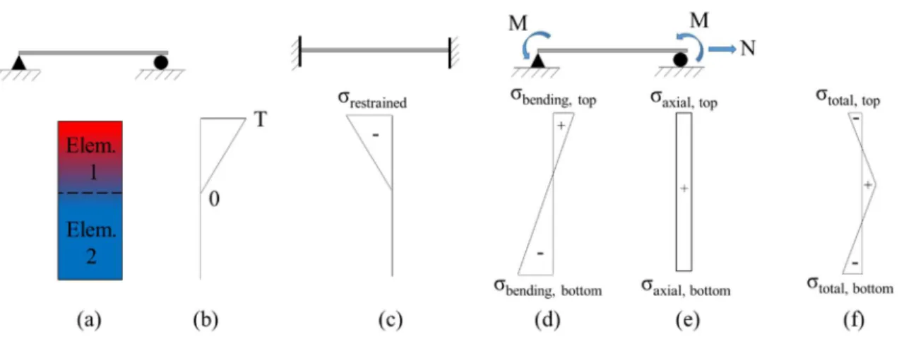
Figure 11: Stress Distributions for Thermal Gradients: a) Structure, b) Temperature Gradient, c) Restrained Stress, d) Bending Stress, e) Axial Stress, and f) Total Stress
Structures in reality are rarely this simple, but the same concept can be applied to more complex systems. For these systems, model calibration through TD St-Id can be used to determine unknown boundary conditions and/or continuity conditions. Once the boundary/continuity conditions have been identified, the structure and its behavior can be analyzed.
5. METHODOLOGY
As mentioned in Section 3, the St-Id method using either the single or multiple model approach can be accomplished with a variety of techniques for modeling, calibration, analysis, etc. This section explains the specific method used for the evaluation of two bridge structures within this study. Finally, an example of the technique is demonstrated on a simple structure exposed to a uniform temperature change.
5.1 Temperature-Driven St-Id using Single and Multiple Model Approach with Bayes Theorem
Overall, the method used in this research for TD St-Id is a probabilistic approach of Latin Hypercube Sampling and Bayes Theorem calibration of finite element structural models. Bayesian techniques have been used for the purpose of structural identification previously (Beck and Katafygiotis 1998; Ravindran et al. 2007). To adequately understand this method, the following sections present the overall process with additional explanation of how the structural evaluation was performed. For completeness, all aspects of the evaluation method are addressed; however, this section primarily focuses on the numerical models and analysis.
5.1.1 Field Experiment
The field experiments conducted for this research were completed according to Steps 1-4 of the SM St-Id process. The specific details of each experiment are discussed in detail later in their respective sections.
5.1.2 Numerical Models 5.1.2.1Model Parameters
The TD structural evaluation process requires a population of structural models with various defining characteristics. The model parameters are chosen based on their potential influence of the behavior of the structure with respect to the load scenario being applied (in this case, thermal loading). As evident from Equations 1-4, changes in many structural characteristics (such as cross-sectional area of bridge member or the properties of the construction materials, to name a few) have the potential to drastically alter the thermal responses of displacement and strain. As a result, these characteristics can be used as model parameters that define the various structural models. Each model parameter is associated with its own set of values (what these values actually are will be discussed later). These values make up what is called the sample space for that parameter.
5.1.2.2Development of Sample Space
For a multi-parameter study, the sample space for the structure becomes an n-th dimensional space, where n is the number of parameters. Imagining an n-th dimensional sample space can be difficult, so plots like the ones shown in Figure 12 through Figure 14 are used as visual aids to understand the sample space more clearly. Plots along the diagonal are histograms of the values of each respective parameter. The remaining plots show a two-dimensional slice of the sample space according to the parameters to the left of each row (y-axis) and below each column (x-(y-axis). Sample spaces for a structure can be developed either deterministically or probabilistically. While each approach has benefits and drawbacks, either can be more efficient depending on the goals and specifics of a particular project. Both approaches are described briefly below.
5.1.2.2.1 Deterministic Approach
The deterministic approach is an iterative, brute force method of sampling the parameters. First, a set of values is assigned to each parameter. Then, the sample space is developed by creating every possible combination of those parameters. An example of this type of sample space can be seen in Figure 12 below. In this figure, each parameter was assigned a set of values ranging from 0 to 100 in increments of 20. The number of samples is determined by the number of parameters and the size of their sets of values. For this scenario with three parameters and six potential values each, the number of combinations (or samples) is equal to 63 or 216.
The deterministic approach is incredibly useful if specific combinations need to be investigated. Also, this method is beneficial for developing the sample space for sensitivity studies, in particular, where one parameter is investigated at a time or compared to other parameters individually. The method can also be used to identify trends that do not need all the information in between but only information at particular intervals. The deterministic approach also has some substantial drawbacks. This method is an iterative process and typically requires more samples, and thus, more time to complete. Also, many samples may be nonsensical as some parameter combinations may produce structural behaviors that do not occur realistically. Another downside of this method is the large areas of parameter combinations that are not sampled. In this example, no samples are developed with values between 0 and 20, 20 and 40, and so on. This aspect significantly limits the application of this approach.
Figure 12: Sample Space of a Deterministic Approach
5.1.2.2.2 Probabilistic Approach
An alternative method of sampling is via a probabilistic approach. Unlike the deterministic method, the probabilistic method is not an iterative process. The number of samples desired is chosen rather than determined from the parameters, and the sample space for the structure is developed based on prior probabilities of each parameter.
Prior Probability Distributions of the Model Parameters
Ideally, structures have minimal uncertainty associated with parameters such as boundary conditions and material properties. In reality, however, these parameters can be difficult to identify with absolute certainty due to the complexity or assembly of the structure as well as the precision of the material manufacturer. In some cases, slight changes in these parameters can drastically alter the model responses. In order to account for these
uncertainties, a probability distribution is applied to each model parameter. For the purpose of better understanding this section, parameter distributions were arbitrarily chosen. Parameters #1 and #2 are normally distributed, and Parameter #3 is uniformly distributed. Once the prior probabilities for each parameter are determined, the sample space is developed by means of Monte Carlo simulations.
Monte Carlo (MC) Simulations
Monte Carlo (MC) simulation is a technique of randomly sampling values within a set domain. Within the probabilistic approach, values are randomly selected based on their respective probability distributions. This selection process determines the parameter combination for each sample before any analysis is conducted. For the parameters mentioned above, Monte Carlo simulations were used to develop the sample space shown in Figure 13 for a total of 500 samples.
Many sampling techniques have been derived from Monte Carlo simulations. One such technique is Markov Chain Monte Carlo (MCMC) simulations. MCMC uses informed decision-making to select the parameters of the sample combinations. In contrast to MC, the sampling and analysis of one sample is completed before the next sample is selected. The information gathered from the analysis of the previous sample is used to determine the parameter combination of the following sample. This process continues until convergence is achieved within all of the parameters. The informed decision-making ability of this technique allows for a smaller sample space thus decreasing computation time. While more efficient than the MC procedure, MCMC is more complicated and computationally involved. Therefore, a simple but efficient MC-derived technique called Latin Hypercube sampling (LHS) is used for this study.
Latin Hypercube Sampling (LHS)
Latin Hypercube Sampling (LHS) is an un-informed sampling technique that retains the defining feature of MC simulations in the fact that the sampling is random; however, LHS methods produce sample spaces that more accurately define the probability distributions of each parameter, as shown in Figure 14. In comparison to Figure 13, notice how the distributions of the LHS sample space in Figure 14 more accurately depict the probability distributions even though both methods use 500 samples. During LHS, the sample space of each parameter is divided into bins and then sampled randomly from within each of those bins. This allows the distributions to be defined more effectively with fewer samples. Furthermore, by implementing this method, a smaller sample space is required, and the time needed for model simulations is reduced. One drawback of the LHS method is that the number of samples needed for a particular project is unknown before conducting the
analysis of the structure. Therefore, a large initial sample size must be chosen at the beginning of the process, and a smaller number of samples required is determined by convergence later. Although not as efficient as the MCMC technique, the LHS technique is a viable option for creating the sample space as it is more efficient than MC and less computationally involved than MCMC. The sample space is then used to develop structural models via finite element analysis.
Figure 14: Sample Space for 500 Samples via Latin Hypercube Sampling (LHS)
5.1.2.3Structural Models via Finite Element Analysis
Once the sample space has been created, the structure must undergo a finite element analysis using the parameter combination from each sample. This task can be a meticulous and time-consuming process, especially if the parameters are addressed manually. However, one way of alleviating these hassles is automation. By using automation, the process has
little need for human intervention, is more efficient, and reduces errors. For this study, the process of automation is made possible by an application programming interface (API) between a programming software (Matlab) and the finite element software (Strand7). The Matlab program sets the model parameters within Strand7 as the parameter combination of the first sample of the sample space. Then, a finite element analysis of the structure is performed. In this case, the linear static solver within Strand7 is utilized to perform this task. Finally, desired structural responses are recorded as output in a results file. The Matlab program repeats the process with the parameter combination of the second sample and continues until all of the samples have completed a finite element analysis to form the structural models.
5.1.3 Single Model Analysis using Bayes Theorem 5.1.3.1Calibrated Model
5.1.3.1.1 Parameter Limits Check
The first task after the results file has been completed is to verify that the measured values are within the ranges of responses from the models. If the measured values are outside of these limits, the model parameters were not chosen properly and need to be adjusted. This result could be indicative of a missing mechanism, meaning an important model parameter was not included in the analysis or the bounds of a parameter were incorrect.
5.1.3.1.2 Posterior Probability for Each Model
Referring back to Figure 2, the ultimate goal of the evaluation process is to identify a structural model or multiple models that behave in a similar manner to a physical structure. For this study, the similarity of the structural models to the physical structure is quantified by their respective posterior probabilities. The posterior probability of each model