Sports Engineering manuscript No. (will be inserted by the editor)
A Three-Dimensional Forward Dynamic Model of the Golf
Swing Optimized for Ball Carry Distance
Daniel Balzerson · Joydeep Banerjee · John McPhee
Received: date / Accepted: date
Abstract A 3D predictive golfer model can be a valu-able tool for investigating the golf swing and designing new clubs. A forward dynamic model, which includes a four degree of freedom golfer model, a flexible shaft based on Rayleigh beam theory, an impulse-momentum impact model and a spin rate dependent aerodynamic ball model, is presented. The input torques for the golfer model are provided by parameterized joint torque gen-erators that have been designed to mimic muscle torque production. These joint torques are optimized to create swings and launch conditions that maximize carry dis-tance. The flexible shaft model allows for continuous bending in the transverse directions, axial twisting of the club and variable shaft stiffness as a function of the length. The completed four-part model with the default parameters is used to estimate the ball carry of a golf swing using a particular club. This model will be use-ful for experimenting with club design parameters to predict their effect on the ball trajectory and carry dis-tance.
Keywords Golf Drive·Forward Dynamics · Simula-tion·Ball Carry·Biomechanics ·Modelling
Daniel Balzerson
University of Waterloo, 200 University Ave. W, Waterloo, ON, Canada, N2L 3G1 Tel.: +1-519-888-4567 x33825 Fax: +1-519-4764791 E-mail: [email protected] Joydeep Banerjee University of Waterloo John McPhee University of Waterloo
1 Introduction & Background 1.1 Motivation
Computer simulations are used extensively in the design of multibody dynamic systems. In the past they have mostly been used for designing the mechanical and elec-trical components of systems, but improved techniques have allowed researchers to begin simulating humans in-teracting with larger systems in biomechatronic models [23]. Simulations of the golf swing have been used since the 1970s [12] to attempt to discover how to play more effectively. By modelling the golfer and club together, we can gain insights into how golfers should swing and the best ways to design their equipment.
Every year there are new claims made by manufac-turers about the performance of new clubs. They claim that ball carry distance can be improved by making the club lighter, increasing the moment of inertia of the clubhead, moving the centre of mass of the clubhead, or any number of other factors that may or may not affect the swing. These claims are difficult to evaluate as human tests are not repeatable and robot tests are not completely bio-fidelic. By constructing a validated computer simulation of the golfer and club, it is possi-ble to test the effect of golf club design parameters on the distance the ball can be struck, reliably and repeat-ably. Some of the questions that the model presented here could answer include: “Do lighter clubs results in longer distances?”, “Where should the centre of mass of the clubhead be located?”, “How does clubheadm mo-ment of inertia affect driving distance?” and “How long should the shaft of the club be?”
The goal of this project was to develop a golf swing model including the golfer and club that can be evalu-ated based on its performance in striking the ball. The
model includes variable parameters for the golfer to al-low for optimization of the swing and variable parame-ters for the golf club to test and evaluate different club designs.
1.2 Previous Golfer Models
Since Cochran and Stobbs initial scientific study of the golf swing in 1968 [3], many further attempts to model the golfer and club have been made. Many inverse dy-namic (diagnostic) studies have been performed where experimental measurements of golfers are used to drive the model and investigate the swing [26][10][2][37][31]. Fewer forward dynamic, or predictive, models of the swing have been developed.
In 1975, Lampsa used optimal control theory to op-timize a torque controlled two-link double-pendulum model of the swing for maximum clubhead speed [12]. Unfortunately, the joint torques produced by that model were dissimilar from those found using inverse dynamics [26]. Pickering and Vickers used the double-pendulum model to examine the release torque at the wrist and found that a natural release of the wrist required the least energy input [29]. More recently, Sharp produced a three-link planar model of the swing that could be optimized by changing parameterized input torques to produce the fastest clubhead speeds [34].
MacKenzie’s model from 2009 also used the concept of parameterized joint torques to improve the feasibility of optimizing the golf swing [15]. His model introduced a fourth degree of freedom to the model golfer allowing for 3-dimensional motion through the supination and pronation of the forearm. This model also included a simple flexible shaft model by dividing the shaft into four rigid sections with a spring and damper at each joint.
There remain significant opportunities for creating an improved golfer model that allows for new questions to be asked and answered. The model presented in this paper incorporates many of the features from previ-ous models along with the following novel elements: a golfer model including active and passive joint torques designed to mimic human muscle; a flexible shaft model that allows for continually varying stiffness parameters along the length of the shaft; and evaluation of each swing using an impact and aerodynamic ball trajectory model.
2 Golf System Model
To simulate the golfer and club and evaluate swings based on ball carry distance, a four-part model of the
Fig. 1 Golfer model with four degrees of freedom indicated
golf swing was constructed. This section will describe each part, its implementation, and its validation.
2.1 Golfer
The golfer portion of the mathematical model consists of three rigid bodies representing the torso, left arm, and left hand of the golfer. There are four degrees of freedom (DoF) for the golfer. The first DoF is the ro-tation of the torso. This represents the roro-tation of the shoulders during the golf swing and is activated by the power of the muscles of the legs and core. The second DoF allows transverse flexion and transverse adduction of the arm across the front of the body. The third DoF allows supination and pronation of the forearm and the final DoF allows for ulnar and radial deviation of the wrist. These four DoF are illustrated in Figure 1. This golfer model, based on the work of MacKenzie [15] was considered to be sufficient to apply the correct kinetics to the club shaft throughout the swing.
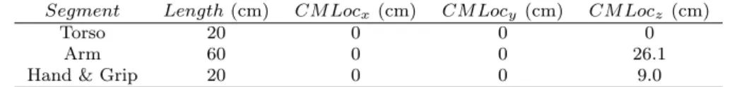
The mass and inertia properties for the torso and arm of the golfer were taken from the work of MacKen-zie [14] and are shown in Table 1. The mass and moment of inertia of the hand also takes into account the mass of the grip of the shaft and is also shown in Table 1. The segment geometries are shown in Table 2. Finally, the golfer’s torso was inclined 30 degrees from the vertical and the swing plane of the arms was inclined 50 degrees from the horizontal. Separate planes of rotation for the shoulder and arm rotation are better able to mimic the swing of a human golfer than single-plane models [8].
2.1.1 Active Torque Inputs
The input torques for the golfer model were defined by the same functions used by MacKenzie [16], taking into account both the activation and force-velocity curves
Table 1 Segment mass properties of the golfer.
Segment M ass(kg) Ixx(kg cm2) Iyy (kg cm2) Izz(kg cm2)
Torso 34.61 ... 3655 ...
Arm 3.431 1076 1096 58.06
Hand & Grip 0.6 10.24 10.24 6.04
Table 2 Segment geometry properties of the golfer.
Segment Length(cm) CM Locx(cm) CM Locy (cm) CM Locz (cm)
Torso 20 0 0 0
Arm 60 0 0 26.1
Hand & Grip 20 0 0 9.0
of human muscles. Each torque generator is controlled by 5 parameters as shown in Table 3. The arm gener-ator provides supination/pronation torques about the long axis of the arm while the shoulder generator pro-vides torque to rotate the arm in the swing plane. The generated torque is calculated as follows.
First, the pre-scaled torque, Tpre(t), is calculated
using Tpre(t) =Tm(1−e ton τa )−Tm(1−e toff τd ) (1)
whereTmis the maximum possible applied torque,τais
the time constant of activation, andτd is the time
con-stant of deactivation. The functionstonandtof fare the
amount of time that has passed since the torque was ac-tivated and deacac-tivated, respectively, and are calculated as piecewise ramp functions:
ton(t) = 0 :t < ta t−tactivate:t > ta (2) tof f(t) = 0 :t < td t−tdeactivate:t > td (3)
where ta is the time at which the joint torque is
acti-vated andtd is the time at which it is deactivated.
Then, the value ofTpre(t) is scaled based on the fact
that muscles cannot exert as much torque on limbs that are already moving quickly. As the angular speed (ω) of the segment increases, the torque provided is decreased based on the following scaling:
T(t, ω) =Tpre(t)
ωmax−ω
ωmax+Γ ω
(4)
This approach was selected because it accounts for both the activation dynamics and the force-velocity relation-ship for the muscles [27] while keeping the number of control parameters small. Since the maximum torque, activation constants, and shape parameters remain con-stant across swings, only the activation timings need to be determined for each torque generator in the model. This results in 8 muscle parameters that must be chosen during the optimization process, two for each DoF.
2.1.2 Passive Joint Torques
As an extension to the model proposed by Mackenzie, passive joint torques are included for the torso, shoul-der, and wrist that represent the energy stored during the backswing. These moments model the passive forces applied by the elastic tissue surrounding the joint at the limits of the range of motion. To model this passive torque, Yamaguchi [38] proposed the use of (5).
Tpassive(θ,θ˙) =k1e−k2(θ−θ−)−k3e−k4(θ+−θ)−c1θ˙ (5)
This function is able to approximate the restoring mo-ment at both extremes of the joint range of motion and offer a smooth transition in joint torque from the normal range of motion, where very little torque is ap-plied, to the large moments applied at the edges. The constantsk1 andk3 govern the magnitude of the force at the breakpoints (θ− andθ+) whilek2andk4govern the sharpness of the break. For this form, θ− and θ+ should be set well within the range of motion of the joint.
For each joint with a passive component, the values
k1,k2,k3,k4,θ−andθ+must be found. A careful search of the literature found explicit values of these parame-ters for ankle, knee, and hip moments [38] [18] [1] but no values for the upper body were found. Instead, the parameters were determined from experimental data [5] [7] [21]. The extracted parameters are given in Table 4. A sample of the fitted curve plotted against the exper-imental for the shoulder data is shown in Figure 2.1.2
2.1.3 Control of the Golfer
By replacing the golfer’s muscle dynamics with param-eterized joint torque functions in the form proposed by MacKenzie [17], control of the swing can be achieved by selecting appropriate values fortactivate andtdeactivate
in (2) and (3). It is assumed that the swing is quick enough that the golfer cannot turn their muscles on and off multiple times during the swing and that the golfer attempts to swing with maximum power. By modifying
Table 3 Parameters for the four active joint torque generators.
Generator Tm(N m) τa(s) τd(s) ωmax (rad s−1) Γ
Torso 200 0.02 0.04 30 4.0
Shoulder 160 0.02 0.04 30 4.0
Forearm 90 0.02 0.04 60 4.0
Wrist 90 0.02 0.04 60 4.0
Table 4 Parameters for passive joint torques at the torso, shoulder, and wrist joints.
Joint θ−(rad) θ+ (rad) k1 k2 k3 k4 c1
Torso 0.0618 -0.693 3.898 2.082 3.814 2.098 0.1 Shoulder -1.289 1.210 2.111 3.354 2.704 2.241 0.1 Wrist -1.171 1.185 4.301 2.732 3.895 2.891 0.1 Forearm -1.237 1.340 3.206 2.624 2.216 1.752 0.1 −3 −2 −1 0 1 2 3 −30 −20 −10 0 10 20 30 40 50 60
Joint Angle (rad)
Passive Moment (Nm)
From Yamaguchi Equation Measured (Engin & Chen, 1986)
Fig. 2 Passive torque for the shoulder joint. The measured experimental torques are marked by crosses and the fitted curve is shown as a solid line.
the relative timings of the joint torque activations, dif-ferent swings can be achieved. The process for selecting the optimal swing parameters for a particular club will be discussed in detail in Section 2.5.
2.1.4 Validation
The golfer model was validated using data from MacKen-zie by using the model to generate a swing similar to that of a human golfer [15]. The model was found to produce angular displacement curves for the torso, shoul-der, arm, and club that well matched the swing of the real golfer given the same initial starting configuration. This matching was performed by using the 8 control pa-rameters for the joint torques along with a scale factor for the maximum joint torque values and angular ve-locities for each joint. Mackenzie’s experiments showed that the four degree of freedom golfer model was able to adapt to match the swings of a human golfer through varying the control parameters. We compared the
mag-Fig. 3 Flexible beam model as proposed by Shi et al. [35]
nitude of the simulated passive forces to the values found in [5] [7] [21] and found good agreement.
2.2 Club
2.2.1 Flexible Shaft
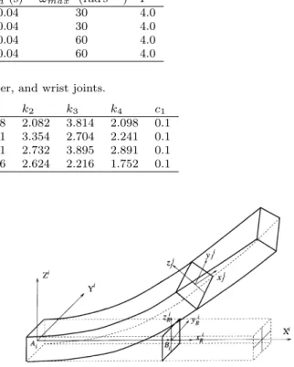
The club model consists of two parts, the flexible shaft and the clubhead. The flexible shaft used in the model is based on the work of Sandhu et al. and a detailed de-scription can be found in [32]. The model uses a flexible Rayleigh beam [35] to describe the flexing and twisting of the club as it is swung. The approach makes use of a complete second-order elastic rotation matrix for a Rayleigh beam and has been implemented in the simu-lation package MapleSim. Shear due to bending is ne-glected, but the model can account for large deflections in the transverse directions and torsion about the shaft that occur during the golf swing. The model can also account for changing stiffness, size, and density of ma-terial along the length of the shaft by defining each as a function of the distance from the bottom of the grip,
x. Figure 3 shows the types of deformations that can be modeled using this type of beam.
The parameters for the flexible shaft,E(stiffness),I
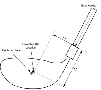
(po-Fig. 4 Front view of clubhead model.
lar moment of inertia), andA(cross-sectional area) are approximated using sixth-order polynomial functions of
x, the distance from the grip. For this work, stiffness for the flexible shaft was provided by a clubhead manufac-turer and polynomials fitting each of the manufacmanufac-turers curves were estimated. The shaft has higher stiffness near the grip and lower stiffness near the clubhead.
2.2.2 Clubhead
The clubhead is modeled as a rigid body fixed to the end of the flexible shaft. The important parameters for the clubhead are the mass, the location of the centre of mass, and the moment of inertia of the clubhead about the vertical axis. These properties were measured for a set of clubheads as part of a different project and one clubhead was selected for initial use in this work. The properties of the selected clubhead are shown in Ta-ble 5. To interpret the location of the centre of mass, Figures 4 and 5 show the corresponding frames of refer-ence. The moment of inertia of the club was measured in a reference frame with the horizontal x-axis out of the face of the club, the vertical y-axis upwards at ad-dress position, and the z-axis away from the golfer (see
xc yc zc in Figures 8 and 9).
Table 5 Clubhead geometry and mass properties ∆X (mm) ∆Y (mm) ∆Z(mm) M ass(g)
40.42 13.2 56.0 200
Fig. 5 Top view of clubhead model.
2.2.3 Club Aerodynamics
The aerodynamics of the clubhead have a small, but not insignificant effect on the swing. Recently, several golf club companies have claimed that they are able to reduce the drag on their clubheads through the addi-tion of small turbulators and other features that change the way the airflow affects the club [6]. To account for aerodynamic effects, drag on the clubhead is included in the model using the standard drag equation:
Fd=−( 1
2ρACd|Vc| 2)Vˆ
c (6)
whereρis the density of the air,Ais the cross-sectional area of the clubhead, andCdis coefficient of drag of the
clubhead.
Measurements ofCdwere provided from experiments
performed in a wind tunnel. A club was placed in the tunnel and rotated from a heel-first presentation to a face-first presentation at a variety of wind speeds. The
Cd value for the clubhead was found to vary with both
the presentation angle of the clubhead and the wind speed. The Cd values for each yaw angle at high
club-head speeds (greater than 33.5 m s−1) are shown in Ta-ble 6. At lower speeds,Cdwas found to be 50 % higher
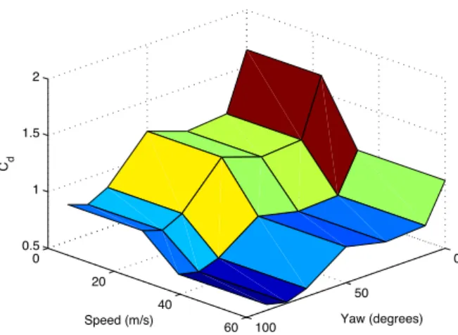
at 22.5 m s−1. The transition zone between high speeds and low speeds is approximated linearly. Figure 6 shows a linear interpolation of the values ofCd for a range of
values of the yaw angle and clubhead speed.
Table 6 Measured values ofCdfor a variety of yaw angles at
high clubhead speeds. A yaw angle of 0 degrees corresponds to a heel-first clubhead presentation (e.g., top of the backswing) while a yaw angle of 90 degrees corresponds to a face-first presentation (e.g., at impact).
Yaw Angle (deg) Cd
0 1.10 10 0.76 30 0.74 50 0.82 70 0.57 80 0.51 90 0.55
0 50 100 0 20 40 60 0.5 1 1.5 2 Yaw (degrees) Speed (m/s) Cd
Fig. 6 Cdvalues for the clubhead as modeled for different
combinations of clubhead speed and yaw angle.
Fig. 7 An illustration of the relevant frames and velocities for calculating the aerodynamic loads on the clubhead.
Since theCdvalue is dependent on both the yaw
an-gle and the velocity of the clubhead relative to the air, we need to define these two variables within the context of the model. This requires the definition of a new coor-dinate system which is body-fixed in the clubhead with the X-axis pointing out of the face, the Y-axis upward along the shaft of the club, and the Z-axis tangent to the club face. We use this coordinate system to define theX−Z plane in which the yaw angle of the club is calculated. To calculate the yaw angle, the velocity of the club is split into two components,vp in theX−Z
plane, and vy normal to the plane. The yaw angle (φ)
is the angle between vp and the −Z axis. The speed
of the airflow used in the calculation ofFd is then vp.
Figure 7 illustrates the both the yaw angle andvp. The
value of Cd at each moment is determined using
Fig-ure 7 and the current values of φand |vp|. Using this
information, we can rewrite our aerodynamic equation as Fd=−( 1 2ρACd(φ,|vp|)|vp| 2)ˆv p. (7)
Finally, the effective cross-sectional area of the club was provided as a constantA = 0.004805 m2 and the density of the air used in the simulations wasρ= 1.1839 kg m−3.
2.2.4 Validation
The flexible shaft model was validated using data from Sandhu et al [32]. Sandhu performed a motion capture experiment with four golfers in order to capture both the grip kinematics and the motion of the clubhead. This experiment captured both grip and clubhead kine-matics of four subjects in order to validate the model of the flexible club. The grip kinematics were then given to the flexible model of the club and the dynamic loft, droop, and clubhead speed compared between the an-alytical model, a finite element model, and the experi-mental data. The analytical model was able to achieve good agreement with the finite element model through-out the swing and good agreement with the experimen-tal results during the impact phase of the swing. The modelled dynamic loft, droop, and clubhead speed at impact were found to be within 10% of the experimental results [32]. The clubhead aerodynamics were compared to experimental data from [6] and found to be in good agreement with the modelled drag force peaking at 6 N compared to wind tunnel measurements of 6.5 N to 9 N.
2.3 Impact
The role of the impact model in this work was to calcu-late the ball launch conditions based on the clubhead velocity, orientation, and angular velocity at impact. The impact model should be realistic, resulting in slice and hook shots for hits with non-ideal clubhead condi-tions. It was important that the impact model simulate quickly as the impact and aerodynamics portion of the model must be used many times within each simulation to determine the optimal timing for striking the ball.
The impact model selected was based on the work of Petersen and McPhee [28] and is a three-dimensional impulse-momentum approach. In calculating the im-pact, the ball and clubhead each have 6 degrees of free-dom and therefore have 6 velocity components following the impact. The three impulses of the impact are also unknown and must be determined, leading to a total of 15 unknowns.
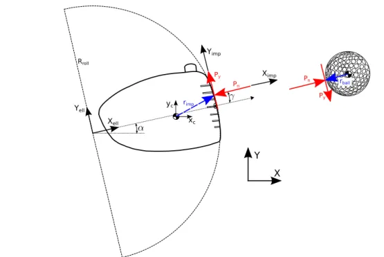
Figure 8 and Figure 9 shows the free body diagram and frames of reference used for developing the impulse
and momentum equations for the clubhead and the ball. There are four relevant reference frames. The first is the global frame (X, Y, Z) in which the clubhead velocity is determined from the swing model and the ball velocity is calculated. For this frame,X is the downrange direc-tion,Y is upwards, andZis outwards away from a right handed golfer. The second reference frame (xc, yc, zc) is
the clubhead frame which is coincident with the global frame when the club is at address position and is body fixed in the club at the centre of mass. The clubhead moments of inertia are defined in this frame. The third reference frame is the ellipsoid frame (xe, ye, ze) which
is used to define an analytical shape for the face of the clubhead. This frame has its origin at the center of an ellipsoid defined by the clubhead’s bulge and roll and is inclined from the clubhead frame by the loft angle (α) of the club so that thexe axis passes through the
centre of face of the club normal to the surface. The final frame of reference is the impact frame (xi, yi, zi)
which is normal to the clubface at the point of impact. The angles γ and β between the ellipsoid frame and the impact frame are caused for an off-centre impact by the bulge and roll of the club and are calculated us-ing the ellipsoid which approximates the surface of the clubface.
The system equations are resolved in the impact frame. By applying the principles of impulse and mo-mentum to the bodies involved, the 12 equations for the clubhead and ball can be written as
mcVc−mcvc=−P (8)
Ic·Ωc−Ic·ωc=rimp× −P (9)
mbVb−mbvb=P (10)
Ib·Ωb−Ib·ωb=rb×P. (11)
In these equations, capital letters stand for the velocity and spin of the ball and club after impact and lower-case letters will be used for the velocity and spin before impact. mc,Ic, mb, andIb represent the mass and
in-ertia tensors for the club and ball respectively.Pis the combined vector of the three impulses,Pn,Pz, andPy.
rimp is the vector from the center of mass of the club
to the impact point in the impact frame, andrb is the
vector from the center of mass of the ball to the impact point in the impact frame.
Three further equations are required to solve for the 15 unknowns. First, assuming the ball rolls without slipping on the face of the club, we have two kinematic constraints that restrict the point of contact on the ball and club to be moving in the same direction at the same speed after impact.
Vcy −Vby = 0 (12)
Vcz−Vbz = 0 (13)
And finally we have the coefficient of restitution equa-tion which accounts for energy lost during the impact due to the deformation of the ball and the vibration of the clubhead.
e=Vcx−Vbx
vcx−vbx
(14)
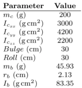
Solving all 15 equations simultaneously, the ball spin and velocity after impact can be found. The required parameters for the impact model can be found in Ta-ble 7.
Table 7 Required clubhead and ball parameters for the im-pact model. Parameter Value mc(g) 200 Icxx (g cm 2) 3000 Icyy (g cm 2) 4200 Iczz (g cm 2) 2200 Bulge(cm) 30 Roll(cm) 30 mb(g) 45.93 rb(cm) 2.13 Ib(g cm2) 83.35 2.3.1 Validation
Validation of the impact model was performed as part of the work of Petersen and McPhee [28]. In this work, the results of impulse-momentum impact model were compared to the results from a finite element model of the ball and club impact. For an impact at the sweet spot of the club, the velocity of the ball after impact was within 6% of the finite element model. Addition-ally, the impact model was compared to results from robot testing performed by Golf Labs. Using impact data from center hits on 4 different clubheads, the im-pact model was found to overestimate the amount of spin on the ball after impact by an average of 9% or about 250 RPM. This is due to the assumption that the ball rolls without slipping on the face of the club. Ball-slip would reduce the gear effect and reduce the spin of the ball. The ball launch velocity was under-predicted by an average of 3.5% or about 5 mph.
2.4 Ball Trajectory Model
After the ball launch velocity and spin has been cal-culated, the ball flight is computed using a trajectory model to allow for comparisons of impacts. By using a trajectory model, it is possible to evaluate the outcome
Rroll Xell Yell xc yc X Y Ximp Yimp rimp Pn Py P n Py rball
Fig. 8 Side view of the impact model illustrating impulses, frames of reference, and the clubhead ellipsoid.
Xell Zell Rbulge xc zc X Z Ximp Zimp rimp Pn Pz Pn Pz rball Shaft axis ΔY CG Location Center of Face
Fig. 9 Top view of impact model illustrating impulses, frames of reference, and the clubhead ellipsoid.
of a golf swing based on an intuitive measure of its suc-cess: the distance the ball travels. This model takes into account the lift, drag, and gravitational forces on the ball in flight. It also includes a decay term for the spin of the ball. A free body diagram of the ball in flight is shown in Figure 10. The aerodynamic model used is based on the work of Quintavalla [30] which provides equations and coefficients for calculating the forces on the ball in flight. It also includes the ability to include wind conditions and elevation data for the tee, but these factors were not included in the model.
The model is simple and uses the usual aerodynamic equations for calculating the lift and drag forces on the
Fig. 10 Free body diagram of the ball in flight.
ball [22]. The coefficientsCD, CL, and CM are
deter-mined experimentally and the values were found to be dependent on the spin rate of the ballSp.
Sp=
ωballD2
Vb
(15)
And the coefficients calculated as follows:
CD= 0.171 + 0.62Sp
CL= 0.083 + 0.885Sp
CM = 0.0125Sp
(16)
whereDis the diameter of the ball, andVbis the speed
of the ball. These values were given in imperial units so a unit conversion was performed before the aerody-namic calculations were performed.
Once the values of the aerodynamic coefficients were determined, the equations of motion for the ball were found by projecting the force equations onto the global coordinate system. The resulting equations of motion for the ball are numerically integrated within Matlab using an explicit Runge-Kutta(4,5) formula to deter-mine the ball trajectory.
2.4.1 Validation
Validation of the ball trajectory model was performed by comparing the results to robot testing data. In this comparison, ball launch conditions from 10 different swings were entered into the aerodynamic model and compared to their actual trajectories from robot test-ing. The mean carry distance was found to be 3.23 m less than the robot testing data with the mean dis-persion distance being only 0.36 m different. The ball model used in this work is from older ball data and could be updated to include modern coefficients if they were available. This would help to resolve the discrep-ancy between the model and the robot testing results.
2.5 Optimal Control
In order for the simulated golfer to adapt to differ-ent situations, it is important to control the swing to produce the best ball carry for each set of simulation parameters used. A human golfer would modify their swing for different clubs, and the simulated golfer should similarly adjust. The optimal control of the golf swing is a difficult problem to solve directly as there are many inputs and biological constraints on the inputs; instead of using conventional optimal control techniques (e.g., Pontryagin’s Minimum Principle or dynamic program-ming) the control of the model was achieved by the selection of parameters for the muscle torque genera-tors.
The optimal control of the golfer model was per-formed through the activation and deactivation tim-ing of the four torque generators in the biomechanical model. From (1) and (3), each torque generator is con-trolled by the timing parameterstactivateandtdeactivate.
Through the selection of these parameters, the opti-mal control of the swing is reduced from a free optiopti-mal control problem with arbitrary torques throughout the duration of the swing to a constrained parameter opti-mization problem.
The objective function is designed to use the most intuitive method for evaluating a swing: by examining the flight path of the ball. The goal is to maximize the distance the ball carries while minimizing the lateral deviation of its flight. The chosen function allows for a
small amount of lateral deviation without a significant penalty to simulate the ball landing in the fairway, but larger deviations are heavily penalized to simulate land-ing in the rough or out of bounds. The equation for the objective function is
M =X−W eZ2/Zmax2 (17)
whereX is the downrange carry,Z is the lateral devi-ation,Zmaxis the maximum acceptable deviation, and
W is a weighting term. The value of Zmax was chosen
to be 4.57 m (5 yards) and the value of W to be 9.14 m (10 yards).
2.5.1 Striking the Ball
One important question remains in choosing the opti-mal parameters for the swing: “Where should the ball be placed by the golfer?” or more accurately within the context of the model: “Where within the swing should the golfer strike the ball?”
To determine the best position within each swing for striking the ball, the simulation examines a range of points within the swing and tests them all to determine which ball position results in the best flight. For every point where the clubhead is within 4 cm of its lowest (approximately 900 points per swing), the impact and aerodynamic analysis is performed and the value of the objective function (17) calculated. The point with the highest value is selected as the ideal point of contact for that swing, and that ball carry and objective function value are considered to be the value for that particular swing. For all impact calculations, the ball is assumed to strike the clubface at the projected CoM location.
2.6 Implementation
The golfer and club model was implemented in Maple-Sim 7 [19]. This program generates the equations for multibody dynamic systems. After implementation, the generated equations were then exported to create a C-function that calculates the velocity and orientation of the clubhead throughout the swing given the mus-cle activations and initial conditions for the golfer’s joints. The integration is performed using a Runge-Kutta solver with a timestep of 10−5seconds. This func-tion was compiled into a.mex function in Matlab [20] where the optimization process was performed. A single swing simulation took around 10 seconds on an 8 core Intel Xeon CPU at 2.13GHz.
A number of different optimization techniques were attempted using Matlab includingfminsearch,patternsearch, and genetic algorithms (ga). In testing, patternsearch
was best able to avoid local minimums and find the global optimum solution. Also,patternsearchallows for simple parallelization as many simulations can be per-formed simultaneously within this scheme. The final optimizations were performed on a high performance computer with 16GB of RAM and 16 available cores at 2.13GHz. A complete optimization run took between 60 and 120 minute depending on the strength of the initial guess and the desired solutions.
Within the optimization, the activation times of the various torque generators were optimized simultane-ously with the starting joint angles for the golfer, for a total of 11 variables within the optimization. These variables along with their constraints and initial guess are shown in Table 8. In addition, the activation of each joint torque was constrained to occur before the deac-tivation. The optimization process was stopped when changes to the activations resulted in less than 1 cm changes to the final carry distance. To increase our con-fidence that a global optimum had been reached, the optimization for the golfer and club configuration pre-sented in this paper was run for a number of different initial guesses which all reached the same final config-uration.
3 Model Limitations
There are many elements of the golf swing that have been intentionally left out of the golfer model to de-crease its complexity. The most obvious omission is the entire lower body of the golfer. The omitted degrees of freedom include the lateral shifting of the pelvis and the independent rotation of the pelvis with respect to the torso. In the context of this model, the removal of hor-izontal shifting seems reasonable because the modern golf swing is primarily a rotational movement. While the golfer feels a significant shift of weight from one leg to the other during the swing, the actual translation of the pelvis is quite small during the swing [13].
The independent rotation of the pelvis has been cited as an indicator of golfer excellence [9] but it is not a degree of freedom that is required to capture the kinematics of the hands of the golfer gripping the club. The rotation of the upper torso will have to start ear-lier if the pelvis rotation is omitted, but the motion of the shoulder joint will remain the same. If the goal of the model was to determine what portion of the power is generated by different joints, this degree of freedom would be important, but since the goal is to evaluate club performance, pelvis rotation can be lumped in with upper torso rotation. This same simplification will also lead to a higher torque for the torso of the golfer as this
torque must provide all of the required angular accel-eration of the arms.
Another omission from the mechanical structure of the model is the omission of the trailing (right) arm of the golfer. The inclusion of this arm would have re-sulted in a closed kinematic loop within the model and complicated the equations that must be solved to de-termine its motion by introducing algebraic constraints to the differential equations. So instead, it is assumed that the golfer’s trailing arm plays a negligible role in providing power to the swing and is simply used for stabilization. Since the model golfer does not need to stabilize the swing (the joints used are inherently sta-ble), the second arm is unnecessary. Since the trailing arm has been removed from the golfer, any power pro-duction from it must be lumped into the leading arm and its strength has been slightly increased. In particu-lar, the pronation-supination strength is required to be larger to close the clubface.
The joint torque model described in Section 2.1.1 describes how the golfer model is activated in a way that approximates the muscles of a real golfer. This approximation of the muscle activity of the golfer sim-plifies the model and reduces the number of parameters that must be optimized to control the swing. A higher fidelity alternative is a model that includes individual muscles attached to a skeletal model of the golfer [23]. However, the inclusion of multiple muscles for each of the joints would require the solution of the muscle re-dundancy problem [4] and greatly increase the length of time required for simulations.
4 Results and Discussion
After running the optimization procedure outlined in Section 2.5, the results for a single representative swing were obtained. The following plots show the large range of swing characteristics that can be examined using this model.
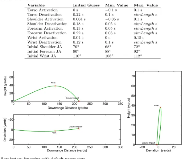
First, the optimized ball carry is 195.7 m (214 yards) with a lateral deviation of 1.8 m. After impact the ball has 3280 rotations per minute (RPM) of backspin, a launch angle of 18.1◦, and a ball speed of 60.8 m s−1 (136 mph). The trajectory results can be found in Fig-ure 11 corresponding to a slight draw. The higher than expected backspin causes a higher arcing trajectory, but this is the best carry result that can be obtained while satisfying the biomechanical constraints on the golfer’s swing.
The clubhead speed is shown in Figure 12. Peak clubhead speed is reached slightly before impact and the clubhead speed at impact is 41.5 m s−1(92.8 mph).
Table 8 List of the 11 variables that are optimized by thepatternsearch and their initial values and constraints.simLength means the end of the simulation time.
Variable Initial Guess Min. Value Max. Value
Torso Activation 0 s −0.1 s 0.1 s Torso Deactivation 0.22 s 0.1 s simLengths Shoulder Activation 0.004 s −0.05 s 0.1 s Shoulder Deactivation 0.18 s 0.05 s simLengths Forearm Activation 0.13 s 0.05 s simLengths Forearm Deactivation 0.22 s 0.05 s simLengths Wrist Activation 0.04 s 0 s 0.15 s Wrist Deactivation 0.12 s 0.1 s simLengths
Initial Shoulder JA 70◦ 68◦ 72◦ Initial Forearm JA 90◦ 88◦ 92◦ Initial Wrist JA 110◦ 108◦ 112◦ 0 50 100 150 200 250 300 350 0 20 40 60 Height (yards) Peak Ground Impact 0 50 100 150 200 250 300 350 20 0 −20
Downrange Distance (yards)
Deviation (yards)
Downrange Distance (yards)
Peak Ground Impact −20 0 20 0 10 20 30 40 50 60 70 Deviation (yards) Height (yards) Peak Ground Impact
Fig. 11 Ball trajectory for swing with default parameters.
This clubhead speed is similar to that observed by Macken-zie, 41.9 m s−1 [16], for a similar model and observed experimentally by Milne & Davis [24]. The clubhead speed at impact is slightly slower than the peak club-head speed to achieve better impact conditions with the ball. By delaying the impact slightly, the club has started to move upwards improving the attack angle of the swing and increasing the launch angle.
Figure 14 shows this delay illustrating how the club is moving upwards at impact (vy >0). Increasing the
delay further decreases the benefit since the clubhead is slowing down and clubhead speed is the most signifi-cant factor in the ball carry distance. The ball is struck near the low point of the swing at a position about 1 m along the z-axis in front of the golfer’s torso. The ball is struck 1.7 cm above the low point of the swing at a legal tee height. The inside-out pattern of the golf drive can also be observed in Figure 14 by noting that the ve-locity in the Z-direction is still positive (moving away from the golfer’s body) at impact. The inside-out pat-tern is suggested by many golf professionals as the best way to hit long straight drives [36]. This pattern also
0 0.05 0.1 0.15 0.2 0.25 0 5 10 15 20 25 30 35 40 45 time(s) Speed (m/s)
Fig. 12 Clubhead centre of mass speed for swing with de-fault parameters.
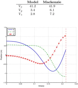
matches the observations of Mackenzie [16] using a sim-ilar model. At impact, Table 9 compares the clubhead speeds at impact of our model to those found in [16]. The velocity in the x-direction is very similar, but our
Table 9 Comparison of clubhead velocity at impact (m s−1) of our model to [16] Model Mackenzie Vx 41.2 41.9 Vy 3.4 6.1 Vz 2.8 7.2 0 0.05 0.1 0.15 0.2 0.25 −1.5 −1 −0.5 0 0.5 1 1.5 time(s) Position (m) X Y Z
Fig. 13 Clubhead centre of mass position
0 0.05 0.1 0.15 0.2 0.25 −30 −20 −10 0 10 20 30 40 50 time(s) Velocity (m/s) X Y Z
Fig. 14 Clubhead centre of mass velocity
velocities in the y and z-directions are quite a bit lower. This is likely because the inclusion of an impact model penalizes high lateral velocity at impact as too high a velocity will result in off-line trajectories.
The golfer’s kinematics are also available from the model. The joint angles are shown in Figure 15. This Figure clearly illustrates the kinematic sequencing of the swing. Att= 0, the torso starts its forward motion, followed by the shoulder around t= 0.05, the wrist at
t = 0.1 and finally the forearm aroundt = 0.15. This progression from the proximal to distal joints is similar to those found in experimental results [25] and previous modeling results [16]. 0 0.05 0.1 0.15 0.2 0.25 −2.5 −2 −1.5 −1 −0.5 0 0.5 1 1.5 2 time(s) Angle (rad) Torso Shoulder Arm Wrist
Fig. 15 Golfer joint angles.
The motion of the forearm degree of freedom is in-teresting and worth discussing further. While the mo-tion of the forearm begins at t = 0.15s the there is significant acceleration in the supination of the arm de-spite declining torque t = 0.17s. This acceleration oc-curs because as the wrist joint brings the club into line with the forearm, the effective moment of inertia of the arm about its long axis is reduced as the mass moves closer to the central axis. The speed of rotation then increases until impact. The combination of the passive and active torques for each joint is shown in Figure 16. This Figure shows the joint torque at each joint peak-ing as the motion begins and fallpeak-ing off as the joint is accelerated.
Figure 17 shows the active portion of the joint torques applied to the model. The torso torque was initiated at t = 0 and peaked at 164 N m which is below the maximum reported in the literature [33]. The shoulder torque was initiated att= 0.022 and peaked at 91 N m which is slightly above the reported value in the litera-ture [11]. This is because the maximum shoulder torque was increased to account for including only the lead arm in the swing model. The wrist torque was initiated at
t = 0.11 and deactivated at t = 0.12. This short ac-tivation is enough to help bring the club in line with the arm for the rest of the swing. Finally the forearm torque is activated to square the clubface at t= 0.14. This torque remains active untilt= 0.17. The sequence of these timings match the experimental timings found in [25].
The model is especially sensitive to changes in the timing of the forearm torque as it is difficult to square the face of the club at impact without precise timing of the forearm torque. Too early a torque will close the face at impact and too late a torque will open the face at
0 0.05 0.1 0.15 0.2 0.25 −100 −50 0 50 100 150 200 time(s) Joint Torque (Nm) Torso Shoulder Arm Wrist
Fig. 16 Total joint torques
0 0.05 0.1 0.15 0.2 0.25 −100 −50 0 50 100 150 200 time(s) Joint Torque (Nm) Torso Shoulder Arm Wrist
Fig. 17 Active portion of joint torques
impact and both of these scenarios lead to large lateral deviations in the ball trajectory.
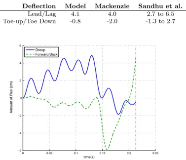
Finally, the model is able to incorporate the flexing and bending of the shaft during the swing. This is easi-est to see in Figure 18. The forward and backward flex-ing of the shaft clearly shows the club bend backwards during the swing and then flex forward for impact. This is the expected result as shown in previous experiments [24]. For the representative golfer and shaft, the club is bent forward 4 cm at impact. The droop oscillates more than expected (possible due to a lack of damping in the shaft model) but does exhibit downward bending (negative droop) at impact. This compares favourably with the experimental results obtained by Sandhu et al. [32] which showed a similar trend in the club droop. Table 10 compares the measured club deflection at im-pact of the model to Mackenzie [16] and experimental results from Sandhu et al.
Table 10 Comparison of club deflection at impact (cm) to [16] and [32]
Deflection Model Mackenzie Sandhu et al.
Lead/Lag 4.1 4.0 2.7 to 6.5 Toe-up/Toe Down -0.8 -2.0 -1.3 to 2.7 0 0.05 0.1 0.15 0.2 0.25 - 6 - 4 - 2 0 2 4 6 time(s) Amount of Flex (cm) Droop Forward/Back
Fig. 18 Club flexing as measured from the grip.
5 Conclusions
A three-dimensional, forward dynamic model of the golfer and club that can be evaluated using ball trajectories computed by an impact and aerodynamics model was created and used to simulate a representative golfer and club. The swing of a simulated golfer is optimized to produce the longest ball carry. In addition to combin-ing four separate models into a scombin-ingle comprehensive model, passive joint forces and club aerodynamics were added to the golfer and club model. The model golfer swings with a clubhead speed of 41.5 m s−1 (92.8 mph) while striking the ball 196 m (214 yards). The model golfer’s joints follow the expected kinematic chain from the torso rotation starting at t = 0s, the shoulder at
t= 0.03s, and the wrist att= 0.12s.
The combined model is a significant contribution to our ability to test golf club design parameters and golf swing biomechanics in simulatio as it could be used to answer many questions of interest in golf club design. By changing the parameters of the club head, the effects of clubhead mass, moment of inertia, and centre of mass position of the clubhead can be investigated. Similarly, other club parameters including the length and stiffness properties of the shaft could be investigated.
Acknowledgements We thank Mike Stachura of Golf Di-gest for providing robot testing results carried out by Gene Parente of Golf Laboratories. Financial support by the Nat-ural Sciences and Engineering Research Council of Canada is also gratefully acknowledged.
References
1. Audu, M., Davy, D.: The influence of muscle model com-plexity in musculoskeletal motion modeling. Journal of biomechanical engineering107(2), 147–57 (1985) 2. Betzler, N.F.: The Effect of Differing Shaft Dynamics on
the Biomechanics of the Golf Swing. Ph.D. thesis, Edin-burgh Napier University (2010)
3. Cochran, A., Stobbs, J.: Search for the Perfect Swing, 2nd edn. Triumph Books, Chicago (2005)
4. Crowninshield, R.D., Brand, R.A.: A physiologically based criterion of muscle force prediction in locomotion. Journal of Biomechanics14(11), 793–801 (1981) 5. Engin, A., Chen, S.M.: Statistical Data Base for the
Biomechanical Properties of the Human Shoulder Com-plex - II:Passive Resistive Properties Beyond the Shoul-der Complex Sinus. Journal of biomechanical engineering
108(3), 222–227 (1986)
6. Henrikson, E., Wood, P., Hart, J.: Experimental inves-tigation of golf driver club head drag reduction through the use of aerodynamic features on the driver crown. Pro-cedia Engineering72, 726–731 (2014)
7. Hirashima, M., Ohgane, K., Kudo, K., Hase, K., Oht-suki, T.: Counteractive relationship between the inter-action torque and muscle torque at the wrist is predes-tined in ball-throwing. Journal of Neurophysiology90(3), 1449–63 (2003)
8. Iwatsubo, T., Adachi, K., Kitagawa, T.: A study of link models for dynamic analysis of swing motion. In: S. Uji-hashi, S.J. Haake (eds.) Engineering of Sport 4, pp. 701– 707. Blackwell Publishing, Kyoto (2002)
9. Joyce, C., Burnett, A., Ball, K.: Methodological consider-ations for the 3D measurement of the X-factor and lower trunk movement in golf. Sports Biomechanics - Inter-national Society of Biomechanics in Sports9(3), 206–21 (2010)
10. Kenny, I.C., McCloy, A.J., Wallace, E.S., Otto, S.R.: Segmental sequencing of kinetic energy in a computer-simulated golf swing. Sports Engineering 11(1), 37–45 (2008)
11. Kuhlman, J., Ianotti, J., Kelly, M., Riegler, F., Gevaert, M., Ergin, T.: Isokinetic and isometric measurement of strength of external rotation and abduction of the shoul-der. Journal of Bone and Joint Surgery74(9), 1320–1333 (1992)
12. Lampsa, M.A.: Maximizing Distance of the Golf Drive: An Optimal Control Study. Journal of Dynamic Systems, Measurement, and Control97(4), 362 (1975)
13. Lindsay, D.M., Mantrop, S., Vandervoort, A.A.: A Re-view of Biomechanical Differences Between Golfers of Varied Skill Levels. International Journal of Sports Sci-ence and Coaching3, 187–197 (2009)
14. MacKenzie, S.J.: Understanding the Role of Shaft Stiff-ness in the Golf Swing. Ph.D. thesis, University of Saskatchewan (2005)
15. MacKenzie, S.J., Sprigings, E.J.: A three-dimensional forward dynamics model of the golf swing. Sports Engi-neering (Springer Science & Business Media B.V.)11(4), 165–175 (2009)
16. MacKenzie, S.J., Sprigings, E.J.: Understanding the role of shaft stiffness in the golf swing. Sports Engineering
12(1), 13–19 (2009)
17. MacKenzie, S.J., Sprigings, E.J.: Understanding the mechanisms of shaft deflection in the golf swing. Sports Engineering12(2), 69–75 (2010)
18. Mansour, J.M., Audu, M.L.: The Passive Elastic Moment at the Knee and its Influence on Human Gait. Journal of Biomechanics19(5), 369–373 (1986)
19. MapleSim: Version 6.4. MapleSoft, Waterloo, ON (2014) 20. MATLAB: Version 8.2.0.701 (R2013b). The MathWorks
Inc., Natick, Massachusetts (2013)
21. McGill, S., Seguin, J., Bennett, G.: Passive stiffness of the lumbar torso in flexion, extension, lateral bending, and axial rotation. Effect of belt wearing and breath holding. Spine19(6), 696–704 (1994)
22. McPhee, J.J., Andrews, G.C.: Effect of sidespin and wind on projectile trajectory, with particular application to golf. American Journal of Physics56(10), 933 (1988) 23. Mehrabi, N., Razavian, R.S., McPhee, J.: A
Physics-Based Musculoskeletal Driver Model to Study Steering Tasks. Journal of Computational and Non-Linear Dy-namics (2014)
24. Milne, R.D., Davis, J.P.: The role of the shaft in the golf swing. Journal of biomechanics25(9), 975–983 (1992) 25. Neal, R., Lumsden, R., Holland, M., Mason, B.: Body
Segment Sequencing and Timing in Golf. International Journal of Sports Science & Coaching2(0), 25–36 (2007) 26. Nesbit, S.M.: A three dimensional kinematic and kinetic study of the golf swing. Journal of Sports Science & Medicine4, 499–519 (2005)
27. Nigg, B.M., Herzog, W.: Biomechanics of the Musculo-skeletal System, 3rd edn. John Wiley & Sons, Chichester (2006)
28. Petersen, W., McPhee, J.: Comparison of Impulse-Momentum and Finite Element Models for Impact be-tween Golf Ball and Clubhead. In: Science and Golf V: Proceedings of the World Scientific Congress of Golf. Phoenix, USA (2008)
29. Pickering, W.M., Vickers, G.T.: On the double pendulum model of the golf swing. Sports Engineering2, 161–172 (1999)
30. Quintavalla, S.J.: A generally applicable model for the aerodynamic behavior of golf balls. In: E. Thain (ed.) Science and Golf IV: Proceedings of the 2002 World Sci-entific Congress of Golf, pp. 341–348. Routledge, St. An-drews, Scotland (2002)
31. Reyes, M., Mittendorf, A.: A Mathematical Swing Model for a Long-Driving Champion. In: M.R. Farrally, A.J. Cochran (eds.) Science and golf III: proceedings of the 1998 World Scientific Congress of Golf, pp. 13–19. Human Kinetics, St. Andrews, Scotland (1999)
32. Sandhu, S., Millard, M., McPhee, J., Brekke, D.: 3D dy-namic modelling and simulation of a golf drive. Procedia Engineering2(2), 3243–3248 (2010)
33. Schultz, a., Cromwell, R., Warwick, D., Andersson, G.: Lumbar trunk muscle use in standing isometric heavy ex-ertions. Journal of orthopaedic research : official publica-tion of the Orthopaedic Research Society5(3), 320–329 (1987). DOI 10.1002/jor.1100050303
34. Sharp, R.S.: On the mechanics of the golf swing. Pro-ceedings of the Royal Society A: Mathematical, Physical and Engineering Sciences465(2102), 551–570 (2009) 35. Shi, P., McPhee, J.: Dynamics of flexible multibody
sys-tems using virtual work and linear graph theory. Multi-body System Dynamics4, 355–381 (1999)
36. Suttie, J.: How to fix a faulty swing path. Golf Magazine
51(8), 55 (2009)
37. Vena, A., Budney, D., Forest, T., Carey, J.: Sports Engi-neering (Springer Science & Business Media B.V.)13(3), 105–123 (2011)
38. Yamaguchi, G.: Dynamic Modeling of Musculoskeletal Motion. Springer Science and Business Media, New York NY (2006)