Retaining principal components for discrete variables

2011, vol. 41, nº 1-3, 33-50 © 2011, Facultat de Psicologia Universitat de Barcelona

Retaining principal components for discrete variables

Antonio Solanas

Rumen Manolov

David Leiva

University of Barcelona

María Marta Richard’s

National University of Mar de Plata, Argentina

The present study discusses retention criteria for principal components analysis (PCA) applied to Likert scale items typical in psychological question-naires. The main aim is to recommend applied researchers to restrain from re-lying only on the eigenvalue-than-one criterion; alternative procedures are suggested for adjusting for sampling error. An additional objective is to add evidence on the consequences of applying this rule when PCA is used with discrete variables. The experimental conditions were studied by means of Monte Carlo sampling including several sample sizes, different number of var-iables and answer alternatives, and four non-normal distributions. The results suggest that even when all the items and thus the underlying dimensions are independent, eigenvalues greater than one are frequent and they can explain up to 80% of the variance in data, meeting the empirical criterion. The conse-quences of using Kaiser’s rule are illustrated with a clinical psychology ex-ample. The size of the eigenvalues resulted to be a function of the sample size and the number of variables, which is also the case for parallel analysis as previous research shows. To enhance the application of alternative criteria, an R package was developed for deciding the number of principal components to retain by means of confidence intervals constructed about the eigenvalues corresponding to lack of relationship between discrete variables.

Keywords: principal components analysis, eigenvalues, parallel analy-sis, discrete items.

*_{This research was partially supported by the Generalitat of Catalonia’s Ministry of Universities, Research and the} Information Society, grant 2009SGR1492.

Correspondencia:Antonio Solanas, Departament de Metodologia de les Ciències del Comportament, Facultat de Psico-logia. Universitat de Barcelona, Passeig de la Vall d’Hebron, 171, 08035, Barcelona. Correo electrónico: [email protected]

Retención de componentes principales para variables discretas

Palabras clave: análisis de componentes principales, autovalores, para-llel analysis, reactivos discretos.

Introduction

Psychological research often deals with understanding the structure of corre-lations among measured variables and even obtaining indirect measurements of underlying dimensions for applied and theoretical purposes. For instance, a psy-chological test assesses anxiety as a construct (or latent variable) by means of observable variables such as the items of a questionnaire referring to physiological measurements, cognitive aspects, etc. Regarding the identification of constructs, it has been argued that exploratory factor analysis (EFA) is the proper statistical procedure for such an aim (Fabrigar, Wegener, MacCallum & Strahan, 1999), at least if there is not enough foundation to specify an a priori model. According to Preacher and MacCallum (2003), an often followed routine in applied and theoret-ical research consists of using a variation of EFA wherein researchers carry out principal components analysis (PCA), retaining components with eigenvalues greater than 1.0, and obtaining new orthogonal dimensions by varimax rotation, a bundle of procedures termed “Little Jiffy”. However, although PCA has been applied in many psychological studies, it is not a reasonable substitute of EFA (Fabrigar et al., 1999; Preacher & MacCallum, 2003). In fact, PCA does not seem

to be a suitable statistical method to identify latent structures since principal compo-nents are linear composites of the measured variables and, thus, include common and unique variance. That is, PCA and EFA have different mathematical models and conceptual meanings and the choice among the two should be based on re-searcher’s aims and on the characteristics of the techniques. The present study focuses on the use of PCA due to the wide use of this statistical technique in ap-plied and theoretical research, although it is not an appropriate substitute of EFA. PCA is a statistical technique applied to a set of measured variables when researchers are concerned with identifying which variables in the set form coher-ent subsets that are independcoher-ent among them. Hence, if the number of measured variables equals p, the specific goal of PCA is to summarise patterns of covari-ances or correlations among variables to a usually smaller number q of underlying dimensions. One of the most difficult decisions that analysts have to make is to choose the number of principal components to retain. In general, researchers us-ing PCA decide on the basis of the absolute and relative size of eigenvalues, alt-hough there are other rules such as including enough principal components to account for, say, 80 percent of the total variance (i.e., the “empirical criterion”) or basing the decision on the graph called “scree plot” (Cattell, 1966). Accordingly, and as a rule-of-thumb, many statistical packages specify a default option in which the number of retained principal components is equal to the quantity of eigenvalues greater than one. This rule, suggested by Kaiser (1960), states that the number of reliable principal components is as large as the number of the existing eigenvalues greater than one. That is, an eigenvalue less than one implies that the scores on the principal component would have negative reliability, although Kai-ser’s reasoning has been shown to be unsuitable (Cliff, 1988). Additionally, the eigenvalues-greater-than-one rule also means that only principal components that account for a greater variance than measured variables do have some summariz-ing power. These rules can be used and specifically adapted when either correla-tion or covariance matrices are used to obtain the eigenvalues.

The eigenvalues-greater-than-one rule may, however, be unsuitable since sam-pling effects may often lead to increasing the number of eigenvalues greater than one. That is, measured variables that are independent among themselves frequently lead to retaining a principal component, although it may not be useful to understand the meaning of the global phenomenon. Zwick and Velicer (1982) studied 48 population correlation matrices and systematically varied the number of measured continuous variables, number of components, sample size, and component saturation. The study showed that the eigenvalues-greater-than-one rule consistently overestimates the number of principal components retained. Interestingly, the number of principal com-ponents retained often fell between one-third and one-fifth of the number of measured variables included in the correlation matrix for low saturation and it increased as the number of measured variables became larger. Hence, it can be argued that in general, the use of the eigenvalues-greater-than-one rule cannot be recommended.

As a potential solution to the overestimation of the number of principal com-ponents, Horn (1965) proposed a statistical procedure, called parallel analysis, for determining the number of principal components to retain. According to this crite-rion, the eigenvalues of a population correlation matrix of independent measured variables are all equal to 1.0. However, if random samples are obtained from such a population correlation matrix, most initial eigenvalues will probably exceed 1.0

whereas the last eigenvalues will be lower than 1.0. Hence, eigenvalues of empirical correlation matrices of p observed variables and n participants should be compared with those obtained from correlation matrices on uncorrelated random data, given that the population matrix corresponds to the identity matrix. Thus, principal com-ponents of empirical correlation matrices for which eigenvalues are significantly greater than those of random correlation matrices would be retained. It should be noted that applying this rule means that researchers are not interested in principal components that do not account for more variance than the corresponding compo-sites from distributions of random and independent numbers. Also note that the rationale can be extended to covariance matrices. It should be mentioned that spe-cific and free software for carrying out parallel analysis in PCA and even EFA is easily available on internet (Patil, Singh, Mishra & Donavan, 2008) and it can be also obtained by well-known computer programs (Ledesma & Valero-Mora, 2007).

It has been found that parallel analysis commonly leads to accurate decisions when applied to PCA (Zwick & Velicer, 1986). Parallel analysis has been studied assuming multinormal distributions or other continuous distribution functions (Dinno, 2009), but Likert scales need to be considered due to their frequent use in applied psychology. Accordingly, recent research has focused on both studying the performance of parallel analysis for binary data (Weng & Cheng, 2005) and adapting it to deal with items with categorical responses (Liu & Rijmen, 2008). Hence, although parallel analysis has also been used for analysing Likert scales (Hayton, Allen & Scarpello, 2004), systematic research on the parallel analysis technique with PCA has to be conducted for this kind of scales, as it is a common procedure in analysing questionnaires.

Statistical descriptive analysis is not sufficient for making inferences to pop-ulations when psychological scales are developed and inferential procedures are needed to obtain statistical significance for eigenvalues. However, in studies where psychological questionnaires require participants to answer items choosing one alternative among the k available and ordered options, the discrete nature of these Likert scales does not allow assuming the observed variables follow a p -variate normal distribution and probably leads to floor and ceiling effects (Nanna & Sawilowsky, 1998). Hence, the asymptotic confidence intervals for eigenvalues and hypothesis testing methods proposed for making statistical decisions are not suitable for most psychological research involving psychometric data analysis. Moreover, asymptotic probability distributions have been mainly derived for the eigenvalues and eigenvectors of a sample covariance matrix (Flury, 1988; Jollife,

1986). Regarding correlation matrices, asymptotic distribution theory of the char-acteristic roots and vectors is more complicated than that of covariance matrices (Morrison, 1976). Due to the reasons mentioned above, it seems that specific sta-tistical tests should be developed to assign stasta-tistical significance to eigenvalues and, thus, make decisions regarding eigenvalues for discrete random variables.

The present investigation focuses on studying the eigenvalues-greater-than-one rule, as we expected that this rule may improperly lead to extract a number of irrelevant principal components for spherical population matrices. This effect can be explained by sampling error if sample correlation matrices are analysed. In addition, the research was also intended to study how that rule may lead to flawed statistical conclusions since its use may suggest retaining an only and artificial principal component for independent observable variables. This fact becomes problematic in those studies in which researchers try to develop one-dimensional scales and are interested in obtaining some empirical support. As applied psy-chometric data are often ordinal level Likert scale data, the simulation study fo-cuses on this sort of measured variables since we were interested in finding some useful results for applied psychological research. Several multivariate techniques, including dimensionality reduction procedures, have already been investigated in relation to non-quantitative variables (Bernaards & Sijtsma, 1999; Ferrando & Lorenzo-Seva, 2001; Jöreskog & Moustaki, 2000; Lee, Song & Lu, 2007; Linting, Meulman, Groenen & van der Kooij, 2007; Meara, Robin & Sireci, 2000; Millsap & Yun-Tein, 2004) and thus the research on such variables is relevant.

Method

Data generation

Given that the objective of the present study was to examine the functioning of PCA applied to psychological measurements, the simulated data consisted of participants by items matrices. Several characteristics of empirical studies were investigated, including the common values available in applied studies. In order to select matrix size simulation values, we carried out a non-systematic review of applied studies1 _{and also considered the findings of previous and more extensive}

studies (Fabrigar et al., 1999; Henson & Roberts, 2006; Weng & Cheng, 2005). Thus, the sample sizes included in the simulation study were 100, 300, 500, 700, and 1000. Our review allowed us to set the number of items to be explored (i.e.,

10, 30, 50, 70, and 100 items). Items were supposed to be answered according to

k-point ordinal scales, whose values ranged from 1 to k. Several values were

tigated for k (3, 4, 5, 6, and 7), representing different intensities of disagreement/ agreement to the items’ statements, as it could have an effect on the decision rules.

For all experimental conditions, data were generated from a population in which the correlation matrix among observed variables was set equal to the identity matrix. That is, the observed variables, which represent items of psychological scales, were supposed to be orthogonal. For each experimental condition defined by the combina-tions of the abovementioned condicombina-tions, data were generated to represent four patterns of items’ mass probability distributions: discrete uniform, discrete triangular, discrete skewed, and mixed. A total of 500 experimental conditions were specified, generating

100,000 data matrices for each of them. A mathematical model was developed to es-tablish the specific probabilities for the discrete distribution functions in order to guarantee some objective criterion. Previous studies were also taken into considera-tion to determine the mass probability funcconsidera-tions to be included in the simulaconsidera-tion study (Micceri, 1989; Nanna & Sawilowsky, 1998; Sawilowsky & Blair, 1992).

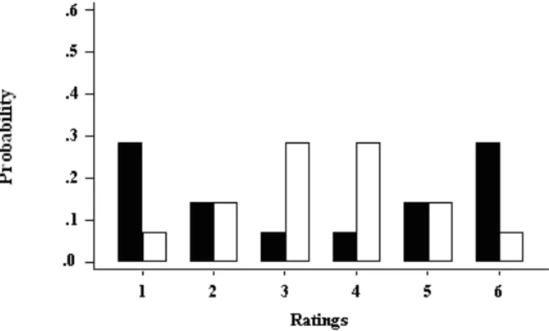
A discrete uniform distribution of answers represents the case where all alter-natives are equally attractive to the participants and the mass probability value of each alternative is equal to 1/k, where k denotes the number of answer options. The mass probability distribution for skewed conditions (figure 1) represents those cases in which alternatives of one extreme are more attractive to the participants. An exam-ple of such a distribution is the case in which each mass probability is equal to twice the previous one when moving towards the heavier tail. For instance, considering the black bars of figure 1, the mass probability of rating 6 is .0159, for rating 5 is twice .0159 and so on until rating 1 where the mass probability is 32 times .0159. For the white bars representing a negatively skewed distribution, the probabilities are the mirror image of the ones for the positively skewed distribution.

Figure 1. Two mass probability functions illustrating positively and negatively skewed distributions.

For discrete triangular distributions, which correspond to symmetric distribu-tions, all items’ mass probability values linearly increased from the extremes to the centre rates (as the white bars show on figure 2). This condition was studied since individuals may avoid extreme answers in favour of more moderate ones. An example of such a distribution is the case in which each mass probability is equal to twice the previous one when moving towards the centre. For instance, considering the white bars of Figure 2, the mass probability of ratings 1 and 6 is approximately .0714285, for rating 2 and 5 it doubles that value and for ratings 3

and 4 it is four times the same value. It is also possible to consider a distribution which is bimodal at the extremes (see the black bars of figure 2). For this distribu-tion, the mass probabilities for rating 1 and 6, on one hand, and for ratings 3 and

4, on the other hand, are inverted with respect to the ones mentioned above. The mixed condition was defined as a combination of discrete uniform, dis-crete triangular, and disdis-crete skewed items’ mass probability functions, different types of items being represented as far as possible by a third of each sort of distri-bution. For questionnaires consisting of 10, 70, and 100 items, the number of them following a discrete uniform distribution was set equal to int(p/3) + 1, where p denotes the number of items. In the case of 50 items, the amount of them which are uniformly and triangularly distributed equalled int(p/3) + 1.

Figure 2. Two mass probability functions showing bimodal at extremes and triangular distributions.

Data analysis

Given that the eigenvalues of population matrices were equal to 1 and the eigenvalues obtained in simulated samples were expected to be close to 1, the empirical eigenvalues were compared to the expected ones. In fact, departures from sphericity were expected due to sampling error.

The fact the items are independent means that the percentage of variance ac-counted for by each principal component should theoretically be equal to 100 divided by the number of items. Hence, the expected variance accounted for by each prin-cipal component was compared to the values obtained in the simulation study.

R and C codes were developed for generating data matrices according to the mass probability functions abovementioned (using the runif R function), to speci-fy correlation matrices, and to obtain eigenvalues (by means of the dsyev Lapack routine). All computations were verified comparing the results to the output pro-vided by common statistical software.

Results

Data features’ influence on eigenvalues

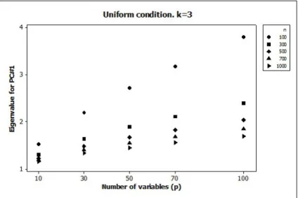
Out of the four factors studied (n, p, k, and type of distribution) only sample size and the number of variables proved to affect eigenvalues. The estimates cor-responding to different number of alternatives only diverge at third decimal, which was also observed in the four distributions studied. Accordingly, the results presented are applicable to all values of k and to all the discrete distribution func-tions studied. As shown on figure 3, a greater number of items are associated with larger first principal component (PC#1) eigenvalues. In contrast, for larger n the eigenvalues corresponding to PC#1 are smaller. The average eigenvalues obtained for each combination of n and p studied are presented in table 1.

Figure 3. Mean eigenvalues for the first principal component (PC#1) for different sample sizes (n) and questionnaire sizes (p). The case of k = 3 alternatives and a uniform distribution is represented.

TABLE1.AVERAGE EIGENVALUE AND PERCENTAGE OF VARIANCE ACCOUNTED FOR BY THE FIRST PRINCIPAL COMPONENT FOR EACH COMBINATION OF N

(NUMBER OF PARTICIPANTS) AND P (NUMBER OF VARIABLES).

Complementarily, the results show that even when the variables are inde-pendent, as much as 50% of the principal components have eigenvalues greater than one (see table 2). In general, it can be seen that an eigenvalue greater than one does not necessarily imply that there is a relationship between the variables and that they can be reasonably summarised by principal components.

TABLE 2.PROPORTION OF PRINCIPAL COMPONENTS HAVING AN EIGENVALUE GREATER THAN ONE (Λ>1) AND VARIANCE ACCOUNTED FOR BY THOSE COMPONENTS FOR EACH

COMBINATION OF N (NUMBER OF PARTICIPANTS) AND P (NUMBER OF VARIABLES). n p =10 p =30 p = 50 p = 70 p = 100 cell content 100 1.530 2.199 2.716 3.172 3.79 eigenvalue

15.30% 7.33% 5.43% 4.53% 3.79% variance accounted for 300 1.295 1.640 1.893 2.111 2.399 eigenvalue

12.95% 5.47% 3.79% 3.02% 2.40% variance accounted for 500 1.226 1.483 1.669 1.827 2.034 eigenvalue

12.26% 4.94% 3.33% 2.61% 2.03% variance accounted for 700 1.190 1.403 1.555 1.683 1.850 eigenvalue

11.19% 4.67% 3.11% 2.40% 1.85% variance accounted for 1000 1.158 1.333 1.457 1.560 1.695 eigenvalue

11.58% 4.44% 2.91% 2.22% 1.69% variance accounted for

n p = 10 p = 30 p = 50 p = 70 p = 100 cell content 100 .5000 .4333 .4200 .4143 .3900 proportion λ > 1

62.60% 66.09% 71.48% 76.26% 80.40% variance accounted for 300 .5000 .4667 .4600 .4429 .4400 proportion λ > 1

57.27% 59.82% 63.09% 64.54% 68.22% variance accounted for 500 .5000 .4667 .4600 .4571 .4500 proportion λ > 1

55.62% 56.85% 59.25% 61.43% 63.80% variance accounted for 700 .5000 .4667 .4800 .4714 .4600 proportion λ > 1

54.75% 55.27% 59.20% 60.43% 61.91% variance accounted for 1000 .5000 .4667 .4800 .4714 .4700 proportion λ > 1

Data features’ influence on the amount of variance accounted for

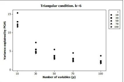
Since the amount of variance accounted for is related to eigenvalues, it varies only as a function of n and p. The amount of variance accounted for by the princi-pal components decreases both for larger samples and for questionnaires with more items, as illustrated on figure 4. For instance, in the case of PC#1 as much as 15% of the information contained in the data can be accounted for when the questionnaire is short (see Table 1). Therefore, the fact that a principal component explains more than 100/p % of the variance should not be taken as an indicator that it has to be retained, since such values can be obtained in presence of random fluctuation. In addition, the amount of variability accounted for by the principal components with λ > 1 ranges from 53% to 80% (table 2), values that can be found frequently in applied studies justifying the principal components retained. In summary, the percentage of variance accounted for may also indicate relevant principal components in presence of independent items.

Figure 4. Variance accounted for by the first principal component (PC#1) for different sample sizes (n) and questionnaire sizes (p). The case of k = 6

alternatives and a triangular distribution is represented.

R code for making decisions on the number of principal components to retain

In order to offer applied psychologists a user-friendly procedure that yields both critical values and confidence intervals, an R package was constructed ( dis-crete_pca, available upon request). Efforts have been made to develop specific

software incorporating the findings of recent research on multivariate techniques (e.g., Kaufman & Dunlap, 2000; Lorenzo-Seva & Ferrando, 2006; O’Connor, 2000). The procedure developed consists of the following steps:

1. Compute the proportions of answers given to each alternative.

2. Generate data matrices of the same size as the original one using the pro-portions obtained in the previous step as mass probability.

3. Compute eigenvalues in the original and the simulated data matrices. 4. Compute the mean and standard deviation of the sampling distribution obtained in the previous step.

5. Print the critical eigenvalue and its corresponding confidence intervals at a specified confidence level.

Therefore, the output of the program helps applied researchers to decide whether to retain a principal component or not, considering the eigenvalues that could have been obtained solely by chance. Regarding the use of the package, once it is installed and loaded in the R working session, it can be used following the steps presented in the Appendix.

An illustrative example of the effects of sampling error

In order to illustrate the inappropriateness of the eigenvalue-greater-than-one rule, the previously presented evidence gathered via simulation will be summa-rised in a contextualised example. Suppose that the psychological inventory of interest is the World Health Organization Disability Assessment Schedule II (WHO-DAS II; World Health Organization, 2000), specifically the shorter 12 -item version, which has not been tested as extensively as the original 36-item instrument. The 12 questions that participants need to answer using a five-point scale (from 1 = none disability during the previous 30 days to 5 = extreme disabil-ity) are: 1. Standing for long periods such as 30 minutes? 2. Taking care of your household responsibilities? 3. Learning a new task, for example, learning how to get to a new place? 4. How much of a problem did you have in joining in com-munity activities (for example, festivities, religious or other activities) in the same way as anyone else can? 5. How much have you been emotionally affected by your health condition? 6. Concentrating on doing something for ten minutes? 7. Walking a long distance such as a kilometre or equivalent? 8. Washing your whole body? 9. Getting dressed? 10. Dealing with people you do not know? 11. Maintaining a friendship? 12. Your day to day work/school?

Although the items have been chosen to represent evenly six different do-mains, it is possible to study how the items group in an exploratory manner until further evidence is available. In fact, there is a recent study (Luciano et al., 2010)

in which exploratory Principal Components Analysis (PCA) followed with an improper oblique rotation is applied to the instrument. Suppose that the results obtained from a sample of 100 participants were the following: 5 eigenvalues greater than one (2.15, 1.53, 1.22, 1.17, and 1.03) with 17.92%, 12.75%, 10.17%,

9.71% and 8.66% variance accounted for, respectively (adding up to a total of

59.21%). Now, suppose that researchers may wish to follow Kaiser’s rule and to

additionally retain a sixth component (whose eigenvalue is .93) given the expecta-tion of the items belonging to 6 subscales (i.e., Understanding and communi-cating, Getting around, Self-care, Getting along with people, Life activities, and Participation in society). In that case, the amounted of variance account for is almost 67%, which could be used as another justification for retaining as many factors.

At that moment, the reader should assess the previous decision on the number of components to retain and their interpretation from the perspective that the 12

variables were actually simulated to be unrelated to each other and, thus, the eigen-values greater than one are only due to sampling error. In the study previously referenced, among the retaining criteria used, Luciano et al. (2010) mention the interpretability of the components, Kaiser’s criterion, and the scree plot. In their study, the PCA yielded two factors with eigenvalues greater than 1.0 (5.54 and

1.22), that accounted for 46.15% and 10.20% of the total variance, respectively. Note that the combined variance accounted for is lower than the one of the five components to be retained (due to sampling error) in the example. The scree plot, however, suggested retaining a single factor, which, in this case, apparently served as a filter for any possible overestimation of the initial eigenvalues, espe-cially for the second principal component (whose eigenvalue in this case coinci-dentally is equal to the one of the third component in the simulated example).

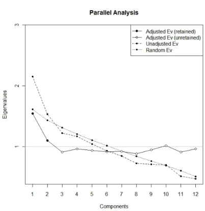
Relying solely on the frequently used eigenvalue-greater-than-one criterion would have led to retaining a second component whose contribution is not un-doubtedly beyond chance levels. In the present simulated example a scree plot can be consulted on figure 5. The original eigenvalues are the unadjusted ones and, in this case, there is no evidence of such drastic difference between the components’ eigenvalues as in the study by Luciano et al. (2010) and so the scree plot would not be as useful.

However, parallel analysis can be used, assessing whether the original eigen-values are greater than the ones expected only by chance. An analyst can proceed in two equivalent ways: a) to retain the components whose unadjusted eigenvalue is greater than the random eigenvalue for the corresponding rank; or b) to retain the components whose adjusted eigenvalue is greater than 1.0. Such decisions can be made via the scree plot on figure 5. In this case, parallel analysis would indi-cate that two components are to be retained instead of five, as the original PCA suggested. The fact that not all the overestimation of the eigenvalues is corrected may be due to the example being an extreme case.

INSERT FIGURE 5 ABOUT HERE

Figure 5. Results obtained via principal components analysis (unadjusted eigenvalues) and parallel analysis (random and adjusted eigenvalues) as applied on a data matrix

with 100 participants and 12 items with 5 alternatives each. The R package paran

(Dinno, 2009) was used to produce the results and the graph.

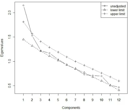
Another alternative is to base the decision on confidence intervals instead of the mean of the random eigenvalues. The limits for the confidence interval for a nominal significance of .05 are represented on figure 6, along with the observed unadjusted eigenvalues. As it can be seen, only the first component’s eigenvalue is clearly beyond what is expected by chance, but the remaining ones are filtered as not significantly different from what is expected for unrelated items. That is, the effects of sampling error are reduced, with the exception of the first eigenval-ue, which is apparently an extreme result. To summarize, it is preferable to use the alternative adjusting for sampling error (i.e., comparing the obtained eigen-values to the expected ones at random or to confidence intervals) rather than the original eigenvalue-greater-than-one rule.

Figure 6. Results obtained via principal components analysis (unadjusted eigenvalues) and confidence interval upper and lower limits obtained through the proposed method

based on Monte Carlo sampling generating 99,999 samples for data matrices with 100 participants and 12 independent items with 5 alternatives each.

The R package discrete_pca was used to produce the results.

Conclusions

The present study focused on the eigenvalue-greater-than-one rule for retaining principal components, as the most frequently used criterion (Henson & Roberts, 2006). A related indicator, the percentage of variance accounted for by the princi-pal components, was also assessed. Both criteria are applied to discrete data rep-resenting participants’ answers to Likert scale psychological questionnaires. The results show that even unrelated variables may lead to eigenvalues and variance accounted for percentages suggestive of retainable principal components. There-fore, alternatives should be considered for retaining components, for instance, comparing the observed eigenvalues with the ones expected by chance and with confidence intervals about these chance values.

The procedure based on confidence intervals that is proposed can be applied through the discrete_pca R package to decide the number of principal

compo-nents to retain which is available upon request from the authors. Confidence in-tervals, as an interval estimator, ensure to a greater extent than point estimators (i.e., the eigenvalues themselves) that the summary variables reflect something more than random fluctuations. Concurringly, for parallel analysis it has been found that the 95th- and 99th-percentile eigenvalues lead to better solutions than mean eigenvalues (Weng & Cheng, 2005). Nevertheless, the eigenvalue criterion can and should be complemented by other decision rules (Thompson & Daniel, 1996), taking into consideration especially the interpretability of the principal components. It is important not to use solely the default options of common statis-tical packages (e.g., the matrix of association used for extraction, the rule for components retention) without a reasonable justification.

Most studies regarding the number of principal components to be retained are concerned with continuous random variables for representing observed measure-ments, as normal and exponential distributions (e.g., Bernstein & Teng, 1998; Peres-Neto, Jackson & Somers, 2005), although psychologists often apply PCA for analy-sing ordinal data. Hence, the present simulation study focussed on questionnaires in which items are answered by Likert scales. The main result obtained shows that using the eigenvalue-greater-than-one rule may often lead to retain trivial axes, that is, un-derlying dimensions from a set of uncorrelated items. The most important explana-tion stems from the fact that principal components are also subjected to sampling error (Larsen & Warne, 2010). Therefore, as it has been previously suggested (Horn, 1965), parallel analysis should be used to prevent from retaining a number of trivial principal components. As regards, applied research can attain some benefit from applying parallel analysis to guarantee that psychological dimensions obtained are not statistical artefacts. However, it must be highlighted that PCA is not an ade-quate statistical technique if psychological researchers are concerned with extract-ing underlyextract-ing psychological dimensions, as EFA is the proper statistical method.

REFERENCES

Bernaards, C.A. & Sijtsma, K. (1999). Factor analysis of multidimensional polytomous item response data suffering from ignorable item nonresponse. Multivariate Behavioral Research, 34, 277-313. Bernstein, I.H. & Teng, G. (1998). Factoring items and factoring scales are different: Spurious evi-dence for multidimensionality due to item categorization. Psychological Bulletin, 105, 467-477. *Byrne, D.G., Davenport, S.C. & Mazanov, J. (2007). Profiles of adolescent stress: The

develop-ment of the adolescent stress questionnaire (ASQ). Journal of Adolescence, 30, 393-416. Cattell, R.B. (1966). The scree test for the number of factors. Multivariate Behavioral Research, 1,

245-276.

Cliff, N. (1988). The eigenvalues-greater-than-one rule and the reliability of components. Psycho-logical Bulletin, 103, 276-279.

*Davey, J., Wishart, D., Freeman, J. & Watson, B. (2007). An application of the driver behaviour questionnaire in an Australian organisational fleet setting. Transportation Research Part F: Traffic Psychology and Behaviour, 10, 11-21.

Dinno, A. (2009). Exploring the sensitivity of Horn’s parallel analysis to the distributional form of random data. Multivariate Behavioral Research, 44, 362-388.

Fabrigar, L.R., Wegener, D.T., MacCallum, R.C. & Strahan, E.J. (1999). Evaluating the use of exploratory factor analysis in psychological research. Psychological Methods, 4, 272-299. Ferrando, P. J. & Lorenzo-Seva, U. (2001). Fitting the normal-ogive factor analytic model to scores

on tests. Multivariate Behavioral Research, 36, 445-469.

Flury, B. (1988). Common principal components and related multivariate models. New York: John Wiley & Sons.

*Ghaderi, A. (2005). Psychometric properties of the Self-concept Questionnaire. European Journal of Psychological Assessment, 21, 139-146.

*Gude, T., Poum, T., Kaldestad, E. & Friis, S. (2000). Inventory of Interpersonal Problems: A three-di-mensional balanced and scalable 48-item version. Journal of Personality Assessment, 74, 296-310. Hayton, J.C., Allen, D.G. & Scarpello, V. (2004). Factor retention decisions in exploratory factor

analysis: A tutorial on parallel analysis. Organizational Research Methods, 7, 191-205. Henson, R.K. & Roberts, J.K. (2006). Use of exploratory factor analysis in published research:

Common errors and some comment on improved practice. Educational and Psychological Measurement, 66, 393-416.

*Hirani, S.P., Pugsley, W.B. & Newman, S.P. (2006). Illness representations of coronary artery disease: An empirical examination of the Illness Perceptions Questionnaire (IPQ) in patients undergoing surgery, angioplasty and medication. British Journal of Health Psychology, 11, 199-220. Horn, J.L. (1965). A rationale and test for the number of factor in factor analysis. Psychometrika,

30, 179-185.

Humphreys, L.G. & Ilgen, D.R. (1969). Note on a criterion for the number of factors. Educational and Psychological Measurement, 29, 571-578.

Jollife, I.T. (1986). Principal component analysis. New York: Springer-Verlag.

Jöreskog, K.G. & Moustaki, I. (2000). Factor analysis of ordinal variables: A comparison of three approaches. Multivariate Behavioral Research, 36, 347-387.

Kaufman, J.D. & Dunlap, W.P. (2000). Determining the number of factors to retain: A Windows-based FORTRAN-IMSL program for parallel analysis. Behavior Research Methods, Instru-ments & Computers, 32, 389-395.

Kaiser, H.F. (1960). The application of electronic computers to factor analysis. Educational and Psychological Measurements, 20, 141-151.

Larsen, R. & Warne, R. (2010). Estimating confidence intervals for eigenvalues in exploratory factor analysis. Behavior Research Methods, 42, 871-876.

Lee, S-Y., Song, X-Y. & Lu, B. (2007). Discriminant analysis using mixed, continuous, dichoto-mous, and ordered categorical variables. Multivariate Behavioral Research, 42, 631-645. Ledesma, R.D. & Valero-Mora, P. (2007). Determining the number of factors to retain in EFA: An

easy-to-use computer program for carrying out parallel analysis. Practical Assessment, Re-search & Evaluation, 12(2). Retrieved from: http://pareonline.net/getvn.asp?v=12&n=2. Linting, M., Meulman, J. J., Groenen, P. J. F., & van der Kooij, A. J. (2007). Stability of nonlinear

principal components analysis: An empirical study using the balanced bootstrap. Psychologi-cal Methods, 12, 359-379.

Liu, O.L. & Rijmen, F. (2008). A modified procedure for parallel analysis for ordered categorical data. Behavior Research Methods, 40, 556-562.

*Loas, G., Yon, V. & Brien, D. (2002). Dimensional structure of the Frankfurt Complaint Question-naire. Comprehensive Psychiatry, 43, 397-403.

Lorenzo-Seva, U. & Ferrando, P.J. (2006). FACTOR: A computer program to fit the exploratory factor analysis model. Behavior Research Methods, 38, 88-91.

Luciano, J.V., Ayuso-Mateos, J.L., Fernández, A., Serrano-Blanco, A., Roca, M. & Haro, J.M. (2010). Psychometric properties of the twelve item World Health Organization Disability

As-sessment Schedule II (WHO-DAS II) in Spanish primary care patients with a first major de-pressive episode. Journal of Affective Disorders, 121, 52-58.

Meara, K., Robin, F. & Sireci, S.G. (2000). Using multidimensional scaling to assess the dimen-sionality of dichotomous item data. Multivariate Behavioral Research, 35, 229-259.

Micceri, T. (1989). The unicorn, the normal curve, and other improbable creatures. Psychological Bulletin, 105, 156-166.

Millsap, R.E. & Yun-Tein, J. (2004). Assessing factorial invariance in ordered-categorical measures.

Multivariate Behavioral Research, 39, 479-515.

Morrison, D.F. (1976). Multivariate statistical methods (2nd ed.). New York: McGraw-Hill. Nanna, M.J. & Sawilowsky, S.S. (1998). Analysis of Likert scale data in disability and medial

reha-bilitation research. Psychological Methods, 3, 55-67.

O’Connor, B.P. (2000). SPSS and SAS programs for determining the number of components using parallel analysis and Velicer’s MAP test. Behavior Research Methods, Instruments & Com-puters, 32, 396-402.

*Oxlad, M., Miller-Lewis, L. & Wade, T.D. (2004). The measurement of coping responses: Validity of the Billings and Moos Coping Checklist. Journal of Psychosomatic Research, 57, 477-484. *Paivio, S.C. & Cramer, K.M. (2004). Factor structure and reliability of the Childhood Trauma

Questionaire in a Canadian undergraduate student sample. Child Abuse & Neglect, 28, 889-904. Patil, V.H., Singh, S.N., Mishra, S. & Donavan, T. (2008). Efficient theory development and factor

retention criteria: Abandon the ‘eigenvalue greater than one’ criterion’. Journal of Business Research, 61, 162-170.

*Pelle, A.J., Denollet, J., Zwisler, A-D. & Pedersen, S. (2009). Overlap and distinctiveness of psy-chological risk factors in patients with ischemic heart disease and chronic heart failure: Are we there yet? Journal of Affective Disorders, 113, 150-156.

Peres-Neto, P.R., Jackson, D.A. & Somers, K.M. (2005). How many principal components? Stop-ping rules for determining the number of non-trivial axes revisited. Computational Statistics & Data Analysis, 49, 974-997.

*Pietrantonio, F., De Gennaro, L., Di Paolo, M.C. & Solano, L. (2003). The Impact of Event Scale: Validation of an Italian version. Journal of Psychosomatic Research, 55, 389-393.

Preacher, K.J. & MacCallum, R.C. (2003). Repairing Tom Swift’s electric factor analysis machine.

Understanding Statistics, 2, 13-43.

Sawilowsky, S.S. & Blair, R.C. (1992). A more realistic look at the robustness and Type II error proper-ties of the t test to departures from population normality. Psychological Bulletin, 111, 352-360. Thompson, B. & Daniel, L.G. (1996). Factor analytic evidence for the construct validity of scores:

A historical overview and some guidelines. Educational and Psychological Measurement, 56, 197-208.

*Vistad, I., Fosså, S., Kristensen, G., Mykletun, A. & Dahl, A. (2007). The Sexual Activity Ques-tionnaire: Psychometric properties and normative data in a Norwegian population sample.

Journal of Women’s Health, 16, 139-148.

*Walsh, T.M., Stewart, S.H., McLaughlin, E. & Comeau, N. (2004). Gender differences in Child-hood Anxiety Sensitivity Index (CASI) dimensions. Anxiety Disorders, 18, 695-706.

Weng, L-J. & Cheng, C-P. (2005). Parallel analysis with unidimensional binary data. Educational and Psychological Measurement, 65, 697-716.

*Wool, C., Cerutti, R., Marquis, P., Cialdella, P. & Hervié, C. (2000). Psychometric validation of two Italian quality of life questionnaires in menopausal women. Maturitas, 35, 129-142. World Health Organization. (2000). Disability Assessment Schedule II (WHO-DAS II). WHO,

Geneva. Retrieved from: http://www.who.int/icidh/whodas/whodasversions/ 12int.pdf. Zwick, W.R. & Velicer, W.F. (1982). Factors influencing four rules for determining the number of

components to retain. Multivariate Behavioral Research, 17, 253-269.

Zwick, W.R. & Velicer, W.F. (1986). Comparison of five rules for determining the number of com-ponents to retain. Psychological Bulletin, 99, 432-442.

APPENDIX

The first required step is to specify the input matrix according a predefined format. If this matrix is in a text file (<filename>), it can be loaded in the working session as follows:

X <- matrix(<filename>,nrow=<number>,ncol=<number>)

where nrow is the number of individuals and ncol is the number of items.

Users have to specify the number of alternatives of the items of the questionnaire (maxinterv) and the number of iterations for the Monte Carlo sampling (rep) as follows:

maxinterv = <number of alternatives> rep = <number between 1 and 10000000>

Researchers can decide whether the program show results for the eigenvectors:

eigenvectors = <TRUE or FALSE>

Finally, the probability of the confidence interval (1 – α) for the eigenvalues has to be choosen (q):

q = < proportion greater than .0 and smaller than 1.>

The function mcpca carries out a Monte Carlo sampling in order to estimate mean and vari-ance for all eigenvalues and the varivari-ance accounted for by them. The function calls a C routine included in discrete_pca that generates rep matrices according to the estimates of probability masses computed by means of the original matrix X: