Entropy-based machine learning algorithms applied to genomics and pattern recognition

(1)

c

(2)

ENTROPY-BASED MACHINE LEARNING ALGORITHMS APPLIED TO GENOMICS

AND PATTERN RECOGNITION

BY

WOOYOUNG MOON

DISSERTATION

Submitted in partial fulfillment of the requirements

for the degree of Doctor of Philosophy in Physics

in the Graduate College of the

University of Illinois at Urbana-Champaign, 2019

Urbana, Illinois

Doctoral Committee:

Professor Karin Dahmen, Chair

Professor Jun S. Song, Director of Research

Assistant Professor Seppe Kuehn

(3)

Abstract

Transcription factors (TF) are proteins that interact with DNA to regulate the transcription of DNA to RNA and play key roles in both healthy and cancerous cells. Thus, gaining a deeper understanding of the biological factors underlying transcription factor (TF) binding specificity is important for understanding the mechanism of oncogenesis. As large, biological datasets become more readily available, machine learning (ML) algorithms have proven to make up an important and useful set of tools for cancer researchers. However, there remain many areas for potential improvements for these ML models, including a higher degree of model interpretability and overall accuracy. In this thesis, we present decision tree (DT) methods applied to DNA sequence analysis that result in highly interpretable and accurate predictions.

We propose a boosted decision tree (BDT) model using the binary counts of important DNA motifs to predict the binding specificity of TFs belonging to the same protein family of binding similar DNA sequences. We then proceed to introduce a novel application of Convolutional Decision Trees (CDT) and demonstrate that this approach has distinct advantages over the BDT modeil while still accurately predicting the binding specificty of TFs. The CDT models are trained using the Cross Entropy (CE) optimization method, a Monte Carlo optimization method based on concepts from information theory related to statistical mechanics. We then further study the CDT model as a general pattern recognition and transfer learning technique and demonstrate that this approach can learn translationally invariant patterns that lead to high classification accuracy while remaining more interpretable and learning higher quality convolutional filters compared to convolutional neural networks (CNN).

(4)

(5)

Acknowledgments

First, I would like to thank my research adviser, Professor Jun Song. He has shown me what it means to be a true mentor and has taught me to be a better researcher, scientist, student, coworker, professional, public speaker, teacher, and leader. He has demonstrated a great amount of patience and sacrifice, which I will always be thankful for.

I would also like to thank the many other educators that have helped me along the way: the members of my thesis and prelim committees, Prof. Seppe Kuehn , Prof. Karin Dahmen, Prof. Patrick Draper, Prof. Sergei Maslov, and Prof. Verena Martinez Outschoorn, for their insightful comments and perspectives; again, Professor Verena Martinez Outschoorn, who gave me the incredible opportunity to work on machine learning at CERN and travel throughout Europe; Prof. Lance Cooper, for his incredibly valuable guidance and kindness through the years; and Dr. John Dell, my high school physics teacher, who first inspired me to pursue physics.

I also sincerely thank the National Brain Tumor Society for their generous financial support.

I am also very thankful for all the Song group members: Alex Finnegan, Yi Zhang, Hu Jin, Chenchao Zhou, Minji Kim, Miroslav Hejna, Mohith Manjunath, Jialu Yan, Alan Luu, Jake Leistico, and Somang Kim, for all of the great conversations and for making the office a safe and enjoyable place to work and learn together. Furthermore, I would also like to thank the close friends in my life, who have been incredibly supportive over the past several years. To name a few in particular: Mazin Khader, Harry Mickalide, Michelle Victora, John Yoritomo, and Ainsley Faux.

Most importantly, I would like to thank my family for their unconditional love and support. This thesis is dedicated to them: my older brother, Joonyoung Moon, who taught me so much growing up together; my father, Ilryong Moon, who has always inspired me to pursue my passions; and my mother, Dr. Haewon Min, who has always been my deepest source of encouragement and comfort.

(6)

List of Tables

4.1 Motif abundances in non-SOX10-associated MITF and MYC-MAX binding sites. . . 39

5.1 Average training accuracy, test accuracy, and their difference for single CDTs trained using the CE method with both normal and grid initialization, simulated annealing (SA), and gradient descent (GD). . . 60

5.2 Average and standard deviation of final loss function values for the head node of CDTs trained using the CE method with both normal and grid initialization, simulated annealing (SA), and gradient descent (GD). . . 62

5.3 Protein-DNA binding prediction scores . . . 64

5.4 BCDT-CNN transfer learning accuracy scores . . . 66

A.1 List of all newly generated sequencing data used . . . 95

A.2 List of all public sequencing data used . . . 95

A.3 List of the most important features used by the Random Forest classifier. . . 95

A.4 Statistics of H3K27ac fold enrichments in all MITF binding sites and Responsive sites. . . 95

(10)

List of Figures

1.1 Central Dogma . . . 2

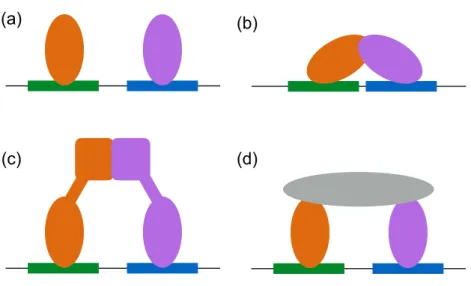
1.2 Mechanisms of cooperative TF (orange and purple) binding. (a) Binding of proximal TFs may cause changes in DNA structure that affect the binding of subsequent TFs. (b) Direct interactions between DNA binding domains, (c) other domains on the TFs, and (d) adaptor proteins (grey) also lead to cooperative TF binding. . . 6

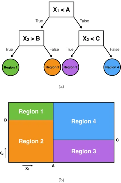
1.3 Univariate decision tree (DT) algorithm overview. (a) DT algorithms can be represented by a tree structure of decision functions. (b) Each leaf node of a DT represents a region in feature space with its own associated output value. . . 8

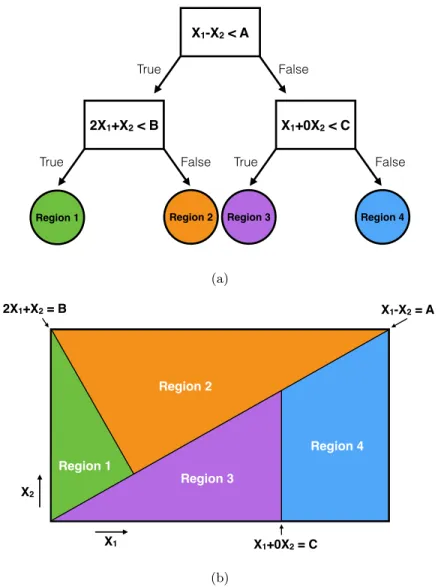
1.4 Oblique decision tree (DT) algorithm overview. (a) Oblique DTs differ from univariate DTs by using a linear combination of features for decision rules at each internal node. (b) The partitions between regions created by an oblique DT are not required to be parallel or per-pendicular to the feature axes. . . 9

3.1 Overview of DNA sequence representations. In the binary motif-count representation,m1. . . mk

denote thekdifferent motifs that are searched for in the DNA sequence. . . 22

3.2 Example of DNA sequence one-hot encoding interpreted as an image. Yellow boxes represent a value of one and purple boxes represent a value of zero. . . 22

4.1 Overview of BCDT interpretation method. . . 35

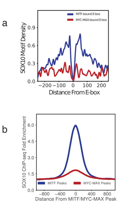
4.2 (a) Density of SOX10 motifs around MITF-bound and MYC-MAX-bound E-boxes. SOX10 motif shows a strong localization 30-150 bps from MITF-bound E-boxes, but does not co-localize with MYC-MAX E-boxes. (b) ChIP-seq read density of SOX10 enrichment around MITF ChIP-seq peaks and MYC-MAX ChIP-seq peaks. . . 38

4.3 Area under the receiver-operating characteristic (ROC) curve for three different models trained to classify between MITF- and MYC-MAX-bound sequences. From left to right: BDT model with bHLH motifs removed; BDT model with full set of motifs; BCDT model.. . . 39

4.4 Distribution of decision function output values for BDT models with bHLH motifs removed (left) and using the full set of motif features (right) demonstrating that sites bound by both MITF and MYC-MAX produce intermediate predictions compared to sites bound by either only MITF or only MYC-MAX.. . . 40

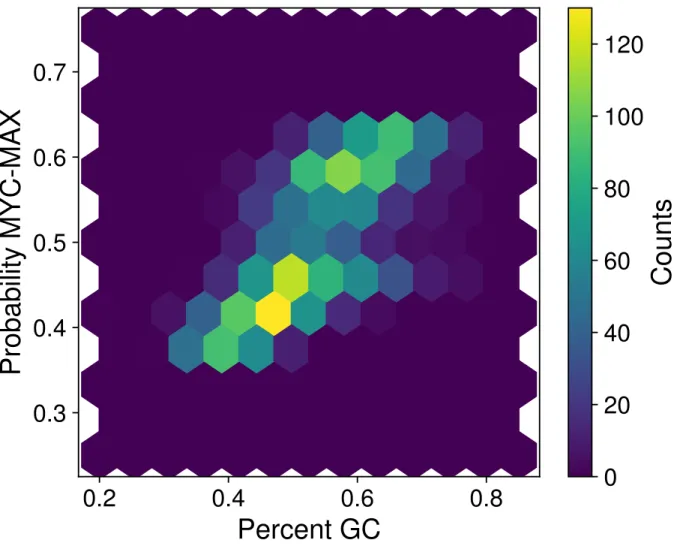
4.5 Density plot showing a positive correlation (Pearson r = 0.70) between percent GC content and the probability of a sequence being MYC-MAX-bound according to our BCDT model trained to classify between MITF- and MYC-MAX-bound sequences.. . . 41

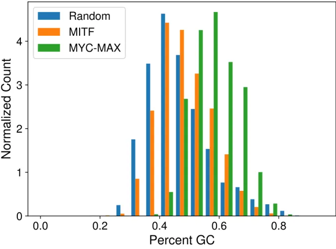
4.6 Normalized histogram of GC content percentage for MITF-bound, MYC-MAX-bound, and random DNase I hypersensitive sequences, demonstrating relative GC enrichment in MYC-MAX-bound sequences. . . 42

(11)

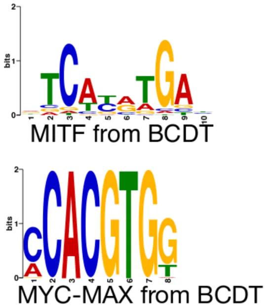
4.7 Visualization of the first CDT of BCDT trained to classify between MITF- and MYC-MAX-bound DNA sequences. The convolutional filterβ at each node is represented by a sequence logo where the height of the letters (A, C, G, T) represents the value of the weight correspond-ing to that nucleotide in the one-hot encodcorrespond-ing representation. The green and red arrows point to the child node that an input sample X is mapped to when a sequence pattern matching the convolutional filter of the parent node is found (green) or not found (red) inX . . . 43

4.8 E-box motifs discovered by the BCDT model in (a) MITF-bound and (b) MYC-MAX-bound sequences. . . 44

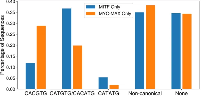
4.9 Bar chart of the fraction of MITF- and MYC-MAX-bound sequences containing the indicated E-box variants. Non-canonical E-boxes were defined using the position-specific scoring ma-trices of MITF and MYC-MAX from Fig. A.3 and TRANSFAC Ebox M01034. This chart demonstrates the relative enrichment of the CATGTG and CACATG motifs in MITF-bound sequences compared to MYC-MAX-bound sequences.. . . 45

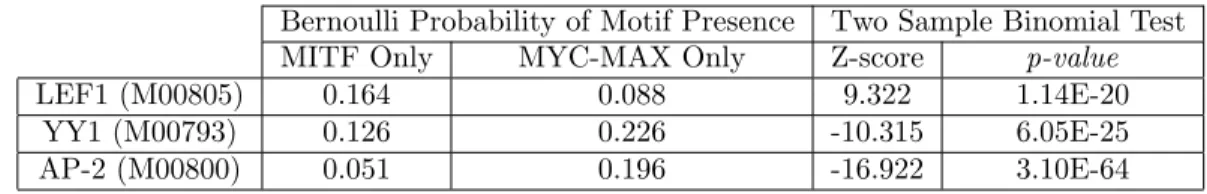
4.10 Partial Dependence plots of eight features having the greatest importance for the BDT mod-els with bHLH motifs removed (left) and using the full set of motif features (right). Positive slopes indicate a positive association between the presence of a particular motif and the mod-els prediction that a sequence is bound by MITF. The relevant TRANSFAC IDs are as fol-lows: (LEF1:M00805), (YY1:M00793), (TP53:M00761), (KLF12:M00468), (E2F-1:M00428), (TFE:M01029), (MYC: M00799). . . 47

4.11 Heatmap of the partial dependence slopes, ordered by slope, of the eight features with greatest importance for the BDT models with bHLH motifs removed (left) and using the full set of motif features (right). Positive (negative) slope values indicate a positive (negative) association between the presence of a particular motif and the models prediction that a sequence is bound by MITF (MYC-MAX). The relevant TRANSFAC IDs are as follows: (LEF1:M00805), (YY1:M00793), (TP53:M00761), (KLF12:M00468), (E2F-1:M00428), (TFE:M01029), (MYC: M00799). . . 48

4.12 Cumulative distribution functions (CDF) of ChIP enrichment in sites bound by MITF showing the percentage of sites with log enrichment scores below a given value. The CDF for sites bound by only MITF (blue) lies above the CDF for sites bound by both MITF and MYC-MAX (orange), suggesting that MITF tends to bind more strongly to the shared sites. . . 50

4.13 E-box motifs discovered by the BCDT model in (a) MITF-bound and (b) MYC-MAX-bound sequences that are non-SOX10-associated . . . 51

4.14 Histogram of BDT decision function output for non-SOX10-associated MYC-MAX-bound sequences that include the MYC-MAX favoring E-box CACGTGG (blue) and the same se-quences with SOX10 motif added in-silico (orange). The rightwards shift in the orange dis-tribution demonstrates that the addition of a SOX10 motif near a MYC-MAX binding site with the MYC-MAX-preferring E-box CACGTGG causes the model to be less certain that the site is in fact bound by MYC-MAX. . . 52

5.1 Schematic overview of the BCDT algorithm.. . . 59

5.2 Boxplots showing classification accuracy scores from CDT optimization method comparison study. The higher median accuracy scores of the CDTs using the CE optimization method demonstrates that using the CE optimization method more consistently leads to more accurate CDT models. . . 61

5.3 Boxplots showing differences between training set and test set classification accuracies from CDT optimization method comparison study. The CE method has the smallest differences between training and test accuracy, suggesting that it learns more biologically relevant con-volutional filters more consistently. . . 61

5.4 Loss function values for head node of CDT trained on ELF1 vs. GABP classification, as a function of optimization iteration for (a) CE method, (b) simulated annealing, and (c) gradient descent averaged over 150 iterations with different, randomized splits of training and test sets. The shaded regions represent the 5th and 9th percentile range of loss function values over the 150 iterations.. . . 63

(12)

5.5 Visualization of the first CDT of BCDT trained to classify between ELF1- and GABP-bound DNA sequences. The convolutional filter β at each node is represented by a sequence logo where the height of the letters (A, C, G, T) represents the value of the weight corresponding to that nucleotide in the one-hot encoding representation. The green and red arrows point to the child node that an input sampleX is mapped to when a sequence pattern matching the convolutional filter of the parent node is found (green) or not found (red) inX . . . 64

5.6 (a) Training and test set accuracies for ELF1 vs. GABP classification, as a function of training epoch for the three different CNN training strategies (Regular, Initialization Only, and Initialization + Freezing) averaged over 200 iterations with different, randomized splits of training and test sets. The shaded regions represent the 5th to 95th percentile range of classification accuracies over the 200 iterations. (b) Difference between the averaged training and test set accuracies as a function of training epoch for the three CNN training strategies. The significantly smaller difference for the Initialization + Freezing strategy suggests a smaller degree of overfitting. . . 66

5.7 Line plot showing the classification accuracies of various models on increasingly translated versions of the MNIST test set. In particular, the BCDT models classification accuracy decays substantially more slowly than the other models tested. . . 67

5.8 Examples of an MNIST test set image of a handwritten “2” with increasing amounts of translation. . . 68

A.1 Bar plot of the ratio of MITF mRNA levels between siMITF and control siRNA-treated cells determined by qPCR in two replicates (qPCR1 and qPCR2) and RNA-seq analysis of the two replicates using Tophat2 and CuffDiff2 [1] (RNA-seq). . . 87

A.2 (a) Distribution of average GC nucleotide frequency in 100 bp windows centered at E-boxes bound by both MITF and MYC and those bound by MITF exclusively. (b) Distribution of average CpG di-nucleotide frequency in 100 bp windows around E-boxes bound by both MITF and MYC and those bound by MITF exclusively. (c) Distinguishing characteristics of the overlapping E-box class, including H3K27ac, H3K4me3 histone modifications, gene expression response to siMITF knockdown, SOX10 co-localization, and E-box evolutionary conservation. Binomial test p-values for testing the difference between the two subclasses of E-boxes are indicated. . . 88

A.3 Motifs of (a) MITF, (b) MYC-MAX, and (c) SOX10 inferred from their respective ChIP-seq data . . . 89

A.4 E-box binding motifs discovered using MEME and DREME, where MITF and MYC-MAX peaks have been split in quintiles according to peak enrichment scores. Quintile 1 is the strongest, and quintile 5 is the weakest. MEME was used in quintiles 1-3 for MITF and quintiles 1-2 for MYC-MAX, while DREME was used for quintiles 4-5 for MITF and quintiles 3-5 for MYC-MAX. DREME was used only in instances where MEME was unable to find a motif. . . 90

A.5 Distribution of MITF and MYC-MAX peaks around transcription start sites (TSS). Both MITF and MYC-MAX show a strong enrichment of peak density around TSS compared to background. . . 91

A.6 Heatmap of log fold-enrichment (normalized to 0 to 1 range) of MITF, MYC-MAX, H3K27ac siCTR, H3Ks7ac siMITF, H3K4me3 siCTR, and H3K4me3 siMITF. Distribution of MITF and MYC-MAX peaks shows a trend of decreasing MITF occupancy with increasing MYC-MAX occupancy and vice versa. . . 92

A.7 (a) UCSC Genome Browser screenshots of representative locations showing binding of MYC-MAX only, (b) MITF and MYC-MYC-MAX co- localized, (c) binding MITF only, and (d) MITF and MYC-MAX sites co-localized with H3K27ac and H3K4me3. COLO829 MAX and MITF tracks show the number of raw sequencing reads after scaling the background noise to Input (Li et al., 2012). H3K27ac and H3K4me3 show fold-enrichment of ChIP-seq signal compared to Input, as determined by MACS2 (Zhang et al., 2008). Black bars beneath each wiggle track indicate the locations of peaks called by MACS2 (Zhang et al., 2008). . . 93

(13)

A.8 Clustering map of MITF, MAX, H3K27ac, and H3K4me3 ChIP-seq read density centered around MITF and MYC-MAX peaks, produced by seqMINER (Ye et al., 2011). MITF ChIP-seq data in melanocyte and 501-mel melanoma cell line are also shown for comparison. . . 94

B.1 Logo visualization of a learned convolutional filter throughout the CE optimization procedure with grid initialization.. . . 99

B.2 Logo visualization of a learned convolutional filter throughout the CE optimization procedure with normal point initialization.. . . 99

B.3 Logo visualization of a learned convolutional filter throughout the gradient descent optimiza-tion procedure. The iteraoptimiza-tion labels are counted in increments of 600 true iteraoptimiza-tions. . . 100

B.4 Logo visualization of a learned convolutional filter throughout the simulated annealing opti-mization procedure. The iteration labels are counted in increments of 500 true iterations. . . 100

B.5 CNN convolutional filters using “Regular” training: Sequence logo representation of all 30 convolutional filters learned by the CNN model trained to classify ELF1- and GABP-bound DNA sequences using the Regular training strategy described in the Results . . . 101

(14)

Chapter 1 Introduction

With the increasing availability of biological datasets and decrease in the cost of computational resources, machine learning (ML) algorithms have proven to be extremely useful tools for the field of genomics. How-ever, despite this progress, understanding the fine details of biological processes such as oncogenesis and cancer progression has proven still to be a difficult task, and much demand remains for improved analytical methods that can help address these problems. The statistical and mathematical nature of both biological systems and ML algorithms place physicists in a position to make contributions to these fields by approaching open questions with a probabilistic optimization perspective often used in statistical mechanics.

1.1 Cancer Biology

Cancer refers to a class of diseases in which abnormal cells divide uncontrollably and invade nearby tissues, often leading to the death of the whole organism. According to the American Cancer Society [2], there were 15.5 million living Americans with a history of cancer in 2016 and 1.7 million new cases are expected to be diagnosed in 2019. Although the rate of cancer-related deaths has steadily decreased 27% from 1991 to 2015 (largely due to a decrease in smoking as well as improved early detection and treatments), a deeper understanding of the genetic causes and mechanisms underlying cancer are important for continuing this trajectory. One particularly promising avenue of cancer genomics research is the application of ML methods to the wide range of large biological datasets that are becoming increasingly more accessible to researchers. Novel biological insights can be extracted from large and noisy datasets using algorithms that automatically learn patterns that may have been difficult for a human to do alone.

For example, ML has proven to be useful for the annotation of genomic elements, during which a ML model learns to identify and distinguish between functional genomic elements (e.g. promoters, enhancers, etc.). In this example, the ML model is trained to do this task by being presented with many examples of putative functional genomic elements, allowing the model to learn the distinguishing patterns and charac-teristics of the various genomic elements. Once the model has learned to perform this task, it can then be

(15)

DNA

RNA

Protein

Replication

Transcription

Translation

Figure 1.1 Central Dogma

used to make predictions on new locations in the genome [3,4,5].

Furthermore, the development of “Next Generation Sequencing” (NGS) technologies has made obtaining genetic and biological data cheaper and faster than ever before, leading to the rapid production of large datasets useful for ML algorithms. In particular, chromatin immunoprecipitation sequencing (ChIP-seq) is a method developed in 2007 [6,7,8] that combines chromatin immunoprecipitation with DNA sequencing, allowing for genome-wide identification of epigenetic modifications and DNA-associated protein-binding sites. Using this type of data, ML techniques have also been used for the prediction of gene expression levels [9], prediction of protein-DNA binding [10], and clustering cancer types [11].

The “Central Dogma” of molecular biology refers to the flow of genetic information within cells. It consists of three major parts: (1) transcription, (2) translation, and (3) DNA replication. Transcription refers to the process by which information stored as DNA becomes transcribed into RNA. Translation refers to the process by which information stored as RNA becomes translated into a sequence of amino acids (i.e. polypeptide), which then folds into a protein. DNA replication refers to the process by which information stored as DNA gets replicated so that daughter cells may have copies of the same DNA information after cell division. Figure1.1shows a simple overview of the three major ideas of the central dogma.

The central dogma plays a central role in almost all cellular functions, and thus, many diseases can be traced back to perturbations in one or more of its steps. For example, improper regulation of the transcription of DNA to RNA can often lead to developing cancer [12]. However, the fine details of the mechanisms of transcription regulation is still an active area of research with many open questions. This thesis focuses on

(16)

the function of proteins that regulate transcription with the ultimate goal of gaining a deeper understanding of how the overproduction or underproduction of these proteins can lead to cancer.

Although the word “cancer” refers to a broad category of diseases with a range of different causes, symptoms, and treatments, Hanahan and Weinberg have defined six common “hallmarks” that nearly all cancers share [13]:

1. Cancer cells stimulate their own growth

Normal tissues control the production and release of signals that promote growth and cell-division in order to maintain a homeostasis of cell number and thus maintain normal tissue function and architecture. In contrast, cancer cells deregulate these signals and acquire the capability for abnormally sustained growth and cell-division.

2. Cancer cells resist signals that are meant to inhibit their growth

Normal tissues react to signals that negatively regulate cell proliferation, often as a result of the action of “tumor suppressor genes.” However, cancer cells often inactivate these signals, leading to an abnormal amount of cell proliferation.

3. Cancer cells resist their own normal programmed cell death mechanisms

Programmed cell death by a process called “apoptosis” as a natural barrier from cancer development is a well-established concept. Cancer cells are often found to have avoided this natural process of apoptosis.

4. Cancer cells can multiply indefinitely

Normal cells have limited replicative potential and eventually reach senescence, a typically irreversible entrance into a nonproliferative state, or crisis, which leads to cell death. Cancer cells go through a transition called immortalization, allowing them to proliferate indefinitely without leading to senes-cence or crisis.

5. Cancer cells stimulate the growth of blood vessels to supply nutrients to the tumor

Like normal cells, cancer cells require a level of nutrients and oxygen as sustenance. In order to grow into a tumor, cancer cells induces “angiogenesis,” causing normally inactive blood vessels to begin sprouting new vessels that carry nutrients into the tumor.

(17)

“Metastasis” refers to the process of cancer cells spreading to and growing in other parts of the body. Understanding the mechanism underlying this process is an extremely important and active area of research due to the significance of cancer metastasis on patient outcomes.

1.2 Transcription Factor Biology

Much of the work within cancer biology is focused on gaining a better understanding of the underlying biological changes that lead to the hallmarks of cancer (Section 1.1) and developing therapies that combat these unwanted cellular behaviors. In particular, understanding the action of transcription factors (TF), proteins that interact with DNA to regulate the transcription of genes, is an area of high interest due to their critical role in maintaining healthy cell behavior [14,15,16]. Thus, significant efforts have been made to understand and characterize the biophysical processes governing the binding and action of TFs [17]. Many TFs function as “master regulators” that sit at the top of a gene regulatory hierarchy and exert control over processes including cell development and differentiation. Since mutations in TFs and their binding sites lead to many diseases, amino acid sequences, physiological roles, and target regulated DNA sequences are often conserved among metazoans [18].

TFs generally bind to DNA in a sequence-specific manner governed by its “DNA-binding domain,” that recognizes and binds specific DNA sequences called “binding motifs.” Extensive work has been done to discover and build databases (such as TRANSFAC [19], JASPAR [20], and UniPROBE [21]) of important TF DNA binding motifs. These DNA binding motifs are represented as position-specific scoring matrices (PSSM) of relative preferences of the TF for each nucleotide position of the binding site. Each of the four bases (A,C,G,T) have a score at each position and multiplying these scores for each base of a given sequence yields a value that represents the relative affinity of a particular TF to the given sequence. Thus, the relative affinity can be written as:

Relative Affinity =Y i

Mi(xi), (1.1)

wherexirefers to the nucleotide in positioniin sequencexandMi(z) is the PSSM value for positioniand nucleotidez.

It is important to note, however, that PSSMs implicitly carry an independence assumption between each position of the DNA binding motif, which has been shown to likely be untrue in many cases [22]. Furthermore, PSSMs do not include any information regarding other important factors such as methylation, cooperative factors, and DNA shape, which have all been shown to be important for predicting TF binding

(18)

[18]. However, despite these shortcomings, PSSMs remain the most popular model for analysis of TF binding. Although TF binding is largely determined by its DNA-binding domain, TFs actually bind only a small fraction of their DNA binding-motifs in the genome [23]. There are many instances of TF binding sites where its predicted binding motif is not present and even more instances of predicted TF binding motifs where the TF does not bindin vivo. This latter situation is often referred to as the “futility theorem” [24], the assertion that “essentially all predicted transcription-factor (TF) binding sites that are generated with models for the binding of individual TFs will have no functional role.” Furthermore, it has been demonstrated that TFs from the same family that share a common DNA-binding domain can still have distinct binding specificities determined by features beyond the TF DNA-binding domains [25].

The concept of cooperative binding provides a good explanation for the TF binding specificity that cannot be explained by DNA binding motifs alone. Cooperative binding is the process by which TFs collaborate in order to aid one another in binding to DNA and carrying out its function in regulating transcription. Studies have demonstrated that cooperative binding of TFs commonly involve the recognition of composite sites that are markedly different from the DNA-binding motifs of the individual TFs [26,27]. TF binding specificity can arise both from physical interactions between coordinating TFs themselves and also from DNA-mediated interactions in which one TF can bind DNA and influence the shape of DNA in a manner that promotes or inhibits the binding of a second TF [28, 18] (Figure 1.2). Furthermore, in addition to cooperative binding, other sources of TF binding specificity are individual TFs having the ability to bind to multiple distinct DNA motifs [29,30], GC composition [29,31], DNA methylation [32], DNA motif flanking sequences [29,33,31], and DNA shape [29,34]. Thus, it is clear that the action and ability of TFs to bind to specific locations is an important area of study because of the important role that TFs play in the regulation of healthy cells and the many open questions that remain regarding their action and regulation.

1.3 Machine Learning

Machine Learning (ML) is the study of algorithms and mathematical models that allow computers to au-tomatically learn to do a task by learning from data instead of being explicitly programmed. One of the earliest examples of ML in practice was demonstrated in 1952 when Arthur Samuel, who was working at International Business Machines Corporation (IBM) at the time and later coined the term “machine learn-ing,” wrote a computer program that played checkers and improved its strategy the more games it played. A few years later in 1957, Frank Rosenblatt designed the first neural network for computers at the Cornell Aeronautical Laboratory [35]. In 1997, IBM’s “Deep Blue” beat world champion Gary Kasparov in a

(19)

best-(a)

_(b)

(c)

(d)

Figure 1.2: Mechanisms of cooperative TF (orange and purple) binding. (a) Binding of proximal TFs may cause changes in DNA structure that affect the binding of subsequent TFs. (b) Direct interactions between DNA binding domains, (c) other domains on the TFs, and (d) adaptor proteins (grey) also lead to cooperative TF binding.

of-six Chess match. In 2016, Google’s “AlphaGo” beat Lee Sedol, a highly ranked professional player, four out of five matches in Go, commonly considered the most complex board game.

The field of ML is often split into two main paradigms, “unsupervised learning” and “supervised learning.” In unsupervised learning, a ML algorithm attempts to find patterns in data without any explicit labels on the individual samples. For example, the authors of [36] identified distinct subtypes of glioblastoma based on just gene expression signatures of cancer cells. Although, the field of unsupervised learning is an exciting and active area of research, this thesis will not be focusing on this particular area of ML and the rest of the discussion will be focused on supervised learning algorithms.

In contrast to unsupervised learning, supervised learning algorithms rely on data in which individual samples have output labels associated with them. A supervised learning algorithm uses a “training dataset” made up of individual input-output sample pairs to learn to approximate how to map a set of input features to an output target value. The output labels in the training set data represent “true” values for the output target values, which the algorithm uses to learn to predict the output values on new samples that are unlabeled. For example, a real estate company may build a model to predict the purchase price of a home based on attributes of that home (e.g. number of bedrooms) by using a training dataset of all previous home purchases in the last decade. In this example, the training dataset is considered labeled because the homes’

(20)

true purchase prices are included in the dataset. Once the model is finished being trained on the labeled data, it can then be used to make predictions on homes that have yet to be sold (i.e. unlabeled samples).

1.4 Decision Trees (DT)

One particularly practical and widely used class of ML algorithms are Decision Trees (DT). DT models are classification and regression algorithms that can be represented by a tree structure consisting of nodes and branches. The internal nodes are defined by decision rules that partition the feature space into disjoint regions and determine the final leaf node with which a given sample input is associated, thereby ultimately resulting in an output value or prediction. Thus, another way to describe a DT is as a series of nested if-then statements resulting in an output value. The most commonly used type of DTs are univariate DTs, which only thresholds a single feature at each internal node to define the decision rule. In contrast, oblique DTs (further discussed in section1.5), are able to use more than a single feature at each internal node at the cost of computational efficiency.

Typically, DTs are built by iteratively partitioning the feature space into disjoint regions such that some measure of the homogeneity of training data in each region is maximized. As a final step, the DT assigns an output value to each feature space partition based on the training set data inside the individual partitions. Predictions are then made by first determining which partition a new inputX belongs to and outputing the value that was assigned to that partition. Additionally, to add more distinguishing power, ensemble methods such as boosting and bagging are often applied to DT models to create boosted decision trees (BDT) and random forests (RF), which have both been widely used in diverse fields including biology, medicine, and particle physics [37,38,39,40]. The popularity and success of DT models may largely be attributed to their interpretability, speed, high level of performance, and ease of training.

Despite these strengths, however, current DT models have several weaknesses as well. One major short-coming is that ordinary DT models have difficulty classifying images from their raw pixel representation. Because ordinary univariate DTs split on individual features one at a time (e.g. individual pixel values in the case of raw images), DT-based models have difficulty learning generalizable or translationally invariant patterns required for robust classification rules. For this reason, DT models are generally used only on pre-processed images where the important features of an image have already been hand-curated or learned using some other method [41,42,43]. In Section3we present a BDT model that follows this idea of using hand-curated features by classifying DNA sequences using short DNA motifs gathered from motif databases. We then subsequently present a novel DT model able to classify DNA sequences by learning motifs directly

(21)

X

1

< A

X

2

> B

X

2

< C

Region 1 Region 2 Region 3 Region 4

True False

True False True False

(a) X1 X2 A B C

Region 1

Region 2

Region 4

Region 3

(b)

Figure 1.3: Univariate decision tree (DT) algorithm overview. (a) DT algorithms can be represented by a tree structure of decision functions. (b) Each leaf node of a DT represents a region in feature space with its own associated output value.

from the data without the need for pre-defined motifs.

1.5 Oblique Decision Trees

In contrast to ordinary univariate DTs, oblique DTs use a linear combination of all available features to make the decision rules at a given node. By doing so, this puts fewer restrictions on the orientation of the boundaries between the partitions in feature space created by the DT algorithm. For comparison, with univariate DTs, the boundaries between the partitions must be parallel or perpendicular to the axes in feature space due to the fact that the decision rules at individual nodes only use a single feature at a time.

(22)

In contrast, for oblique DTs, the boundaries between partitions no longer have that restriction and can be oriented in a diagonal direction (Figure1.3vs. Figure1.4).

X1-X2 < A

2X1+X2 < B X1+0X2 < C

Region 1 Region 2 Region 3 Region 4

True False

True False True False

(a) X1 X2 Region 4 Region 2 Region 1 Region 3 X1-X2 = A 2X1+X2 = B X1+0X2 = C (b)

Figure 1.4: Oblique decision tree (DT) algorithm overview. (a) Oblique DTs differ from univariate DTs by using a linear combination of features for decision rules at each internal node. (b) The partitions between regions created by an oblique DT are not required to be parallel or perpendicular to the feature axes.

It has been shown that adding this extra flexibility to the decision rules at each node or an oblique DT results in smaller and more accurate trees when compared to univariate DTs [44]. However, a major challenge in training an oblique DT is the time complexity of finding the optimal oblique split at a given node. Specifically, for a training set of n samples and p features, the time complexity for an exhaustive search for the best fit at any given node isO(2p n

p

) while it is justO(np) for an axis-parallel split [45]. The authors of [46] are one of the earliest to propose a method of inducing models from data that resemble oblique DTs by defining and splitting on “linear transgeneration units” that can be interpreted as

(23)

linear combinations of the inputs. Classification and Regression Trees - Linear Combination (CART-LC) [47] is often considered the first major oblique DT induction algorithm, which used a hill-climbing algorithm to search for the best oblique split at a given internal node. A weakness of CARL-LC is that there is no built-in mechanism to avoid getting trapped in local minima during optimization. To address this difficulty, Simulated Annealing Decision Tree (SADT) [48] uses the simulated annealing optimization algorithm to search for optimal splitting. The OC1 algorithm [45] combines ideas from both CART-LC and SADT by using a hill-climbing algorithm with randomization steps incorporated to avoid local minima. MIO-H [49] casts the training of a DT as a single mixed integer optimization problem instead of building the tree in a greedy manner. APDT [50] use the Aloplex optimization algorithm to optimize for “degree of linear separability” instead of sample homogeneity within nodes. Evolutionary algorithms have also proven useful and efficient method for the induction of oblique DT splits [51,52,53].

In addition to developing new optimization techniques to build oblique DTs, standard statistical tech-niques have also been used to create oblique splits in a DT. Fisher’s Decision Tree [54], QUEST [55], Ltree [56], Discriminant Trees [57], Fisher’s Sequential Classifiers [58], and the algorithm presented in [44] are based on linear discriminant analysis. LMDT [59] solves a set of discriminant functions at each that are collectively used to assign each sample to a class. Other oblique DT training procedures have included the use of logistic regression [60] and support vector machines [61,62].

Heuristics have also been used to avoid the need for the costly optimization procedures required in the previously mentioned examples. The HOT heuristics [63] create oblique splits using projects on a vector that is produced by joining the centroids of two adjacent regions discovered by a univariate DT. HHCart [64] and CARTopt [65] reflect samples using Householder matrices and then use axis-parallel splits on the reflected samples. The authors of [66] train a neural network with a single hidden layer and use the hidden unit activations to build a univariate DT. BUTIA [62] uses a “bottom-up” approach and employs an EM-based clustering algorithm to generate the initial leaves and then SVM to generate the splitting hyperplanes.

In this thesis, we demonstrate how the cross entropy (CE) method, a stochastic optimization algorithm inspired from rare-event simulation and based on concepts related to statistical mechanics, can be used to train a novel variant of an oblique decision tree called a convolutional decision tree (CDT). In Section5, we present the results of comparison studies, demonstrating how the CE optimization method can lead to more accurate CDT models compared to other common optimization algorithms.

(24)

1.6 DTs applied to images

Tree-based methods, including univariate DTs [67, 68, 69], RFs [70, 71, 72, 73], BDTs [74, 75, 76], and oblique DTs [77, 69, 78] have been used for image segmentation of remote sensing data where individual pixels are classified based on data from multiple different types of sensors (e.g. infrared cameras, RADAR, etc.). Similarly, [79] used pixel-wise image features such as gray-scale and local variation for general image mining and segmentation.

In 2014, the authors of [80] proposed Convolutional Decision Trees (CDT), a particular instance of an oblique decision tree, as an accelerated method for feature learning and image segmentation. In their method, a quasi-newton optimization algorithm is used to learn convolutional filters that classify individual pixels as belonging to a certain class. Despite the previous work that has applied tree-based algorithms to image-related tasks, tree-based models have yet to be effectively used for pattern recognition and whole-image classification based on raw pixel values. The BCDT approach that we introduce in Section 3 and use in Sections4 and5extends the concepts from Laptev’s CDT model originally used for image segmentation to classify whole images based solely on their raw pixel values.

1.7 Computer Vision and Neural Networks

Convolutional Neural Networks (CNN) attempt to solve the problem of learning translationally invariant patterns by using convolutional and pooling layers. The convolutional layers convolve a learned filter across an image to create a “feature map,” while the pooling layers define spatial neighborhoods on the feature map to consolidate and reduce its dimensionality by performing an operation such as keeping the maximum value within the pooling neighborhood, referred to as “max-pooling”. With the use of these principles, CNNs have produced state-of-the-art performance in various computer-vision tasks, such as image classification [81] and object detection [82].

Despite these strengths in performance, it has been demonstrated that CNNs are not actually transla-tionally invariant and that their outputs are sensitive to even small image translations and transformations [83, 84]. In addition to this lack of true translational invariance, CNNs often remain as black-box models, and developing methods for their interpretation is currently an active area of research [85,86]. Furthermore, deep neural networks with many hidden layers are notoriously difficult to train [87] and often require a great amount of expertise and experience to choose an architecture, tune hyperparameters, initialize weights correctly, and avoid the “vanishing gradient” and “exploding gradient” problems where the gradients for weights in early layers of a deep neural network become very close to zero or diverge to very large values

(25)

making training difficult. An additional drawback is that a CNN also requires the user to pre-specify the size of images to be modeled; consequently, any images of a different size must be re-sized accordingly to fit the specific pre-defined architecture of the CNN. The CDT model introduced in Section 3 addresses many of these weaknesses of CNN by using a much simpler model architecture with fewer hyperparameter choices, incorporating full translational invariance, and allowing for both training and testing on variable sized inputs. Section5 presents further discussion on these advantages of CDTs over CNNs.

1.8 Overview

Here, we present a BDT-based approach to understanding the binding specificity of TFs from the same family and show how such an approach can be used to accurately predict protein-DNA interactions and produce biological insight about the factors that lead to the binding specificity. We also present a novel application of Boosted Convolutional Decision Trees (BCDT) trained with the Cross Entropy (CE) optimization method that addresses many of the weaknesses of ordinary DT models and CNNs by using fully translationally invariant convolutional filters in a tree-like structure. We demonstrate that BCDT learns informative and interpretable convolutional filters, corresponding to DNA sequence motifs, that can be transferred to CNNs to improve their performance. We also demonstrate that BCDT is more robust against image translations compared to other models by applying the model to the well-known MNIST handwritten digit classification dataset and comparing the BCDT performance with other popular ML models.

The structure of the rest of this thesis is as follows: in Section2, we provide further theoretical background on topics that will be important for the reader to understand the methods and analyses presented in our studies. In Section3, we introduce general methods used in the analyses presented in Sections4 and5. In Section4, we demonstrate how DT models can be used to answer questions regarding TF binding specificity and present the results from our paper [10]. In Section5, we present further studies on the BCDT algorithm as a general pattern recognition technique and demonstrate its advantages over competing algorithms. Finally, in Section6, we conclude with an overview of our results and provide thoughts on potential areas for future studies.

(26)

Chapter 2 Theoretical Background

In this section, we present further background on key concepts that will be useful to the reader for the purpose of understanding the methods used and results in latter sections. We begin with an overview of the process of training a supervised ML algorithm. We then present mathematical details of DTs and boosting. Finally, we conclude with details regarding the CE optimization method.

2.1 Training ML Models

In the supervised learning paradigm, a modelF learns to approximate a function that maps a set of input “features” X to an output “target” y based on a set of input-output pair examples called the “training dataset.”

Parametric ML algorithms are ones in which a certain functional form of the model is assumed and the behavior of the model Fβ is parameterized by a set of parameters β. Parametric ML algorithms are useful because the behavior of the model Fβ is completely determined by its parameters β and thus, the burden of defining a model is reduced to choosing the optimal set of parameters. This process of choosing the optimal parameters is called “training” the ML model and is generally carried out with the following steps: (1) building the “training dataset,” (2) defining a loss function, and (3) choosing and carrying out an optimization algorithm to find the optimal set of parameters.

Building the training dataset generally involves splitting the available labeled data into a set of samples that the model will use to optimize its parameters and a different non-overlapping set of samples called the “test dataset” that is used post-training to test or validate the performance of the model. Additionally, sometimes a third set of samples called the “validation dataset” is partitioned for the purpose of validating a trained model without exposing it yet to the test set. Since the test and validation sets are used to assess how the model will perform on new, unseen samples, it is important that these sets of data have no overlap with the training set and each other.

(27)

target values. A loss function can generally be written as:

Loss =L( ˆy,y) (2.1)

ˆ

y= (F(X0), F(X1), . . . , F(XN)) (2.2)

y= (y0, y1, . . . , yN) (2.3)

and are designed to take on lesser values when the model’s outputs are more desirable. In the case of ML algorithms such as logistic regression and neural networks, the loss function is often a measure of model accuracy. Examples of such loss functions include mean squared error loss and negative log likelihood loss. Thus, a model that minimizes a loss function measuring accuracy is effectively attempting to minimize its errors. In contrast, DTs often use a loss function that measures sample heterogeneity in its internal nodes. Thus, DTs do not necessarily search for the set of parameters that minimize error, but instead attempt to maximize node homogeneity.

The next step in training a ML model is to choose and implement an optimization method to search the space of model parameters to find an optimal point β∗ _{that minimizes the chosen loss function. This}

problem can be stated as:

β∗= argmax β

L(Fβ(Xtrain),ytrain), (2.4) whereFβ(Xtrain) andytrain are the predicted and true output values for the training dataset, respectively.

In the case of simpler models such as logistic regression, the number of trainable parameters can be as low asp+ 1, wherepis the dimensionality of a sample’s input feature vectorX. However, more complex models such as neural networks can include thousands or even millions of trainable parameters. Thus, choosing a proper and efficient method of optimizing for the loss function over such a high dimensional parameter space is paramount to successful training of a ML model. A full review of optimization methods used in ML is out of the scope of this thesis, but a more comprehensive review on common optimization procedures used in ML may be found at [88].

A final and optional step for training a ML model is to tune “hyperparameters.” Hyperparameters are parameters of a ML model that is external to the model and are not estimated from the training dataset. Instead, they are chosen prior to the model being trained and affect the structure of the model as a whole. Hyperparameter tuning is often carried out by training many different models with different hyperaprameter values on the same training set and choosing the set of hyperparameters that lead to the best performance

(28)

on the validation dataset. Once the hyperparameters have been decided upon on this way, the model can be tested on the test dataset to obtain an estimate of the model’s true performance. The reason for choosing the hyparparameter values based on a validation set separate from the test set is to avoid an inflated estimate of model performance by potentially simply choosing the hyperparameter values that happen to lead to the best results on that particular test dataset.

2.2 Decision Trees (DT)

A DT modelFmaps a sampleXto an output target valueyby traversing through a series of nodes applying branching rules, ultimately resulting in a final output value determined by the terminal leaf node assigned to a sample. The decision rule at each node is defined by a function f(X), which takes a sample X as its argument and outputs a value which determines to which child node the sample gets assigned to. Each internal node has its own associated branching rule and a sample traverses down the tree by these branching rules until reaching a terminal leaf node, which has an associated output value instead of a branching rule. For example, in a univariate decision tree, which splits the data at each node using a single feature at a time, the decision function at a given node can be written as:

funi(X) =1(X(i)_{> T}₎_, _(2.5)

where X(i) _{is the} _i_{-th element of} _X _and _T _{is a threshold parameter. All samples that lead to an output} value of zero are then mapped to one child node while all samples that lead to an output value of one are mapped to the other child node.

The most commonly used training algorithms for decision trees learn the decision rules in a greedy manner, choosing the most optimal split at each node by maximizing some measure of homogeneity in the training samples assigned to the child nodes. The main disadvantage of training DTs in a greedy manner is that the algorithm generally searches for locally optimal (as opposed to globally optimal) parameters. The trade-off for searching for local optima is that these greedy methods are much more computationally efficient. Efficient, greedy algorithms such as ID3 [89], C4.5 [90], and CART [47] have allowed for fast training of classification and regression trees, largely contributing to the rise in popularity of DT models.

For classification trees, the measure of homogeneity can generally be written in terms of the sum of sample weights of each class in each of the child nodes.

(29)

ny,c= X i∈{j|Cj=c} wi1(yi=y), (2.6) nc= X y∈Y ny,c, (2.7) py,c= ny,c nc , (2.8)

The Gini indexGand Shannon entropy H are common measure of homogeneity used for training clas-sification trees and can be written in terms of thepy,c andnterms.

G= X c∈{L,R} _n_c nL+nR X y∈Y py,c(1−py,c) (2.9) H = X c∈{L,R} _n_c nL+nR X y∈Y

−py,clog(py,c) (2.10)

For regression trees, the mean squared error (MSE) and mean absolute error (MAE) are commonly used measures of homogeneity. nc= X i∈{j|Cj=c} wi (2.11) yc= 1 nc X i∈{j|Cj=c} wiyi (2.12) MSE = X c∈{L,R} _n_c nL+nR _X i∈{j|Cj=c} (yi−yc) 2 _(2.13) MAE = X c∈{L,R} _n_c nL+nR _X i∈{j|Cj=c} |yi−yc| (2.14)

DT models contain many hyperparameters that can greatly affect the performance of the model. The maximum depth of a decision tree determines when to stop building the decision tree. If no maximum depth is set prior to building a DT, the algorithm will build the DT until every node’s homogeneity of training samples is maximal (i.e. each child node is made up of samples from a single class). Since this may lead to an undesirable degree of overfitting, setting a maximum depth is often used to limit the DT training from getting to that point.

(30)

Algorithm 1Greedy DT Learning

1: Initialize empty stack data structureS 2: Push root node to stack S

3: while S not emptydo

4: nodeN ←pop head node from stackS 5: if Stopping criterion not met on node N then

6: Search for optimal branching rule that maximizes child node homogeneity 7: Push child nodes ofN to stackS

2.3 Boosting

Boosting refers to a class of meta-algorithms that iteratively creates an ensemble of “weak learners,” resulting in a “strong learner.” A weak learner is defined as a predictive model that is only slightly correlated with the true target value. In contrast, a strong learner is one that is highly correlated with the true target value. Most commonly, simple DT models with a small maximum depth are used as the weak learners that combined into an ensemble to make a strong learner called a Boosted Decision Tree (BDT).

A distinguishing characteristic of boosting compared to other ensemble methods such as bagging and stacking is the sequential manner by which it is carried out. In general, boosting algorithms train individual weak learners to correct the errors made by the previous weak learners in the ensemble. Consequently, the

i-th weak learner can only be trained once the 1, . . . ,(i−1)-th weak learners have been trained, making boosting algorithms intrinsically difficult to parallelize.

Two commonly used boosting algorithms are Adaboost and Gradient Boosting. Although it can be shown that Adaboost is equivalent to a special case of Gradient Boosting using an exponential loss function, the two algorithms are described here as distinct algorithms. In Adaboost, new weak learners are trained to correct the errors made by the existing weak learners by up-weighting training samples that were misclassified by the existing weak learners and down-weighting training samples that were correctly classified by the existing weak learners. By doing so, the loss function used to train the next weak learner will be more dominated by the samples with higher weights and thus, the new weak learner will attempt to fit the previously misclassified samples more strongly. In contrast, in Gradient Boosting, no changes are made to the sample weights. Instead, new weak learners are trained to fit the errors or residuals of the existing weak learners. Thus, instead of changing the weights and leaving alone the target values of the samples, Gradient boosting changes the target values and leaves alone the weights of the samples.

(31)

Algorithm 2Adaboost

1: Initialize the observation weights wi= 1/N, i= 1,2, . . . , N

2: form= 1, M do

3: Fit classifierGm(x) using weightswi. 4: Compute: errm= PN i wiI(yi6=Gm(x)) PN i wi

5: αm= log((1−errm)/errm)

6: wi←wi·exp(αm·I(yi 6=Gm(x)), i= 1,2, . . . , N.

7: G(x) =PM_m=1αmGm(x)

Algorithm 3Gradient Boosting

1: Initializef0(x) = argminγPN_i=1L(yi, γ)

2: form= 1, M do

3: rim=−[∂L(y_∂f(xi,f(xi)

i) ]f=fm−1, i= 1,2, . . . , N 4: Fit modelf∗(x) to the targetsrim

5: fi(x)←fi−1(x) +f∗(x)

6: F(x) =fM(x)

2.4 Cross Entropy (CE) Method

The Cross Entropy (CE) method [91] was originally proposed for rare-event sampling and was later adapted as an optimization algorithm for finding globally optimal solutions in non-convex optimization problems. The CE method relies on the minimization of the KullbackLeibler (KL) divergence, a common distance measure used in information theory that has been shown to be closely related to the maximum work available during the relaxation process of a system out of equilibrium (i.e. the “exergy” of a system) [92]. Based on the principle of importance sampling, the CE method searches for globally optimal parameter values by iteratively sampling points from a parametric distribution that gradually becomes more sharply centered around the optimal values. More precisely, at thei-th sampling step,M points in parameter space are drawn from a multivariate normal distribution G(µi,σi) estimated from the previous step. Subsequently, the loss function (for DT models, the loss function is some measure of label homogeneity of nodes) is computed for each of theM sets of parameter values, and only the topppercent of theM points is kept, while the rest is discarded. Finally, the new distribution G(µi+1,σi+1) for the next iteration is calculated by taking a weighted average of the current parameters (µi andσi) and the maximum likelihood estimates (µMLEi and σ_iMLE) obtained from using only the top points:

(32)

µi+1=αµMLEi + (1−α)µi, (2.15)

σi+1=ασMLEi + (1−α)σi, (2.16)

where αis a hyperparameter that takes a value between 0 and 1.

Algorithm 4Ordinary CE method

1: functionfind optimal filter(N, M, n, α, σinitial)

2: σ←σinitial1

3: µ←Random initialization

4: fori←1, N do

5: samples list =Sample Multivariate Normal(µ,σ, M)

6: top samples list =_{Get Top Scoring}(samples list, n) 7: µMLE_,_σMLE_←_MLE_{(top samples list)}

8: µ=αµMLE_{+ (1}₋_α₎_µ

9: σ=ασMLE_{+ (1}₋_α₎_σ

(33)

Chapter 3 General Methods

In this section, we present general methods used in the analyses presented in Section 4 and Section5. We begin by describing the different representations for DNA sequences used in later analyses. We then provide details regarding the BDT models and the different methods used to interpret those BDT models. We then introduce a novel application of convolutional decision trees (CDT) and the modified cross entropy (CE) optimization used to train CDT. Finally, we present a brief discussion regarding the major hyperparameters and model choices for CDT and

3.1 DNA sequence representation

The DNA sequences used for the ML models were represented in two ways: (1) One-hot encoding and (2) Binary motif counts. The one-hot encoding representation can be considered a raw representation of the DNA sequence, virtually equivalent to the DNA sequence string itself. In contrast, the binary motif counts represents a more processed and abstract representation of the DNA sequence where the presence or absence of pre-defined, important sequence patterns and motifs define a given DNA sequence.

3.1.1 Motif counts

In order to encode information regarding potential proteins and co-factors bound to a given DNA sequence, binary motif counts were chosen as a practical representation for DNA sequences. PSSMs representing TF motifs from the TRANSFAC [19] Human and JASPAR [20] databases were used to build a total of 435 binary features, each feature representing either the presence or absence of one of the 450 motifs in the given DNA sequence.

The natural questions that follows is: given a PSSM for a given motif and a DNA sequence X, how should X be labeled as either an instance of the PSSM or not? This process is often referred to as “motif calling.” One possible method is to take the highest probability nucleotide from each position/row of the PSSM to form a single stringsthat defines the motif and then to search the DNA sequenceX for an exact

(34)

match with s. However, this definition of the presence of a motif doesn’t take into account the fact that TFs can often bind to multiple similar sequences and thus, only considering a single particular string as the motif that the TF binds to may be too strict of a requirement. Furthermore, the different positions of a TF binding motif often have different levels of flexibility in terms of deviating froms. Thus, in order to address these weaknesses, we model the DNA sequences with a third-order Markov model and use an information theoretic approach for motif calling.

For a DNA sequenceX of lengthL, PSSM probability distributionP, and third-order background prob-ability distributionQ, the log likelihood ratioLof observing sequenceX under the probability distributions of P and Q was calculated. This log likelihood ratio was then thresholded using the relative entropy D

betweenP andQacross sequenceX. IfL is greater thanD, we considerX to be an instance of the motif defined by PSSMP. L(X) =X i logP(Xi) Q(Xi) (3.1) D(X) =X i Q(Xi) logP(Xi) Q(Xi) (3.2) The relative entropy can also be interpreted as the expected value of the log likelihood ratio under the background probability distribution. Thus, the intuition behind using the relative entropy as a thresh-old becomes clear; a log likelihood value greater than the one expected under the background probability distribution suggests that sequence X is more likely to have been generated by P than the background distribution.

3.1.2 One-hot encoding

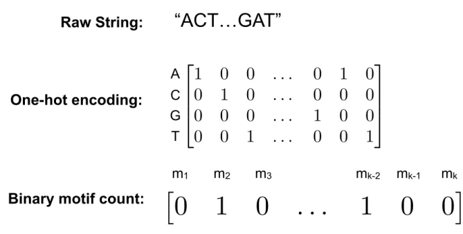
In order to use a DNA sequence representation that is more unbiased than using binary counts of predefined motifs, the one-hot encoding representation of DNA sequences were used. In this representation, a DNA sequence of length L was transformed into a 4×L matrix of 1’s and 0’s. In the one-hot encoding matrix representation, each column represents the nucleotide at a given position along the sequence and each row represents one of the four nucleotides (A, C, G, T).

Xi,j=        1, if nucleotide at positionj isN(i) 0, otherwise (3.3)

(35)

“ACT…GAT”

Raw String:

⇥

0

1

0 . . .

1

0

0 ⇤

m

1

m

2

m

3

m

k-2

m

k-1

m

k

2

6

4 1 0 0

. . .

0 1 0

. . .

0 0 0

. . .

1 0 0

0 0 1

. . .

0 0 1

3

7

5 A

C

G

T

One-hot encoding:

Binary motif count:

Figure 3.1: Overview of DNA sequence representations. In the binary motif-count representation,m1. . . mk denote thekdifferent motifs that are searched for in the DNA sequence.

Sequence Position

A C G T

Figure 3.2: Example of DNA sequence one-hot encoding interpreted as an image. Yellow boxes represent a value of one and purple boxes represent a value of zero.

Note that the resulting matrix can be treated as a two dimensional image of size 4×Lor a one dimen-sional image with four channels of length L (Figure 3.2). Thus, both standard and novel image/pattern recognition techniques can be used to classify sequences represented in this way. An overview of the different representations of DNA sequences is shown in Figure3.1.

3.2 Boosted Decision Trees (BDT) with Motif Counts

Using the binary motif count features, boosted decision tree models trained to classify between DNA se-quences bound by different TFs from the same family were built using the scikit-learn implementation of gradient boosted decision trees [93].

(36)

3.3 BDT Interpretation

An important advantage of DT models compared with others is their relative interpretability compared to other ML models. For a single DT of reasonably low depth, one is able to visually look at the tree structure and decision rules at each node making up the DT to understand what the model has learned. However, this is no longer the case once ensemble methods such as boosting and bagging have been applied to create BDT and RF models, which often consist of hundreds and even thousands of single DTs. Thus, it is important that there are other methods for the interpretation of these ensembles of DTs.

3.3.1 Feature Importances

Often when training a ML model, it is of high interest to know the relative importances of the available features for the construction of a given model. BDT feature importances can be estimated using the relative amounts that each feature reduced the impurity measure in the individual DTs making up the whole BDT model. Thus, for DT modeltand featurel, the importance scoreIl(t) is defined as

Il(t) = X n:Nl

i(n), (3.4)

where NL is the set of all nodes splitting on featureland i(n) is the improvement in measure of homo-geneity between that node and its child nodes. As previously mentioned this measure of homohomo-geneity is up to the user to choose, but examples include Gini index, shannon entropy, and mean squared error.

For an ensemble E of DTs, the importance score of feature l is calculated by taking a average of its importance score across all the individual DTs, weighted by the ensemble weight of each DT.

Il(E) = 1 W X t wtIl(t) (3.5) W =X t wt (3.6)

3.3.2 Partial Dependence

Once the most important features have been identified, it is often of great interest to understand how the BDT model’s output depends on the identified most important features. Partial dependence (PD) plots are a visual representation of the marginal effect that a set of features have on the output of a ML model. Since PD plots are generally inspected visually, the set of features usually consists of just one or two features. For

(37)

our description of partial dependence, we follow the same notation used in [94].

Consider the full input vector X = (X1, X2, . . . , Xp) of dimensionp, subvectorXS made up of l < pof the original features indexed by S ⊂ {1,2, . . . , p}, and subvector XC indexed byC, the complement of S, such thatS∪C={1,2, . . . , p}. The partial dependence of the modelf(X) onXS is defined as:

fS(XS) =EXC(f(XS,XC)) (3.7)

Equation 3.7 represents the marginal average of the model output f, which can be interpreted as the effect of the XS on f after accounting for the average effects ofXC onf. Note that this is not the same as the effect ofXS onf ignoring the effects ofXC altogether. PD plots are a general method that can be applied to any ML model, but is most often used with DTs due to a particularly efficient way of computing the PD plots in the context of DT models.

3.4 Convolutional Decision Trees (CDT)

A key weakness in using binary motif counts as features for distinguishing between different types of DNA sequences is that the approach requires a curated list of biologically relevant motifs to be available in the first place. Although this happens to be true in the case of TF motifs (e.g. TRANSFAC and JASPAR databases), this may not always be true in every situation, so a more general method that can learn the biologically relevant motifs on its own with minimal prior information is desired. Additionally, there is a level of bias introduced when using a binary counts of a predetermined set of motifs. Thus, a more agnostic method would alleviate concerns relating to this type of bias.

In order to address these concerns, we developed a novel application of Convolutional Decision Trees (CDT) for image classification and pattern recognition and applied it to DNA sequence classification and later test the novel model on the popular MNIST handwritten digit classification dataset. The code for CDT, which runs on Python 3.6, is available athttps://github.com/wmoon5/ConvDT.

CDT is a classification and regression DT model that uses learned, translationally invariant convolutional filters to define the decision rules at each internal node. More precisely, at nodekwith a convolutional filter

βk of fixed size (w1,w2), the following decision function is evaluated for each sample:

fβk(X) = max_i,j 1(βk·Xi:i+w1,j:j+w2> T) (3.8) where X is the full data matrix encoding the sample, Xi:i+w1,j:j+w2 is the submatrix of X with rows i

Entropy-based machine learning algorithms applied to genomics and pattern recognition