Passivity and synchronization of coupled complex-valued memristive neural networks

(1)

Passivity and Synchronization of Coupled

Complex-Valued Memristive Neural Networks*

1

st

Yanli Huang, 2

nd

Jie Hou

Tianjin Key Laboratory of Optoelectronic Detection Technology and System School of Computer Science and Technology

Tiangong University

Tianjin 300387, China

[email protected], JHou [email protected]

3

rd

Shunyan Ren

School of Mechanical Engineering Tiangong University Tianjin 300387, China [email protected]

4

th

Erfu Yang

Department of Design, Manufacture and Engineering Management

Faculty of Engineering University of Strathclyde

Glasgow G1 1XJ, Scotland, UK [email protected]

Abstract—The coupled complex-valued memristive neural net-works (CCVMNNs) are investigated in this study. First, we analyze the passivity of the proposed network model by designing an appropriate controller and using certain inequalities as well as Lyapunov functional method, and provide a passivity condition for the considered CCVMNNs. In addition, a criterion for guaranteeing synchronization of this kind of network is established. Finally, the effectiveness and correctness of the acquired theoretical results are verified by a numerical example. Index Terms—memristive neural networks, synchronization, passivity, state coupling

I. INTRODUCTION

Recently, coupled neural networks (CNNs) have been widely concerned owning to their extensive application in secure communication, chaos generator design, brain science, etc. As we all know, these applications heavily depend on the dynamic behaviors of CNNs, especially the synchronization and passivity of CNNs [1]–[5]. In [2], the impulsive synchro-nization of Markovian jumping randomly CNNs was consid-ered by using multiple integral approach. Some conditions for guaranteeing synchronization of CNNs were obtained in [3]. Ren et al. [5] analyzed the passivity of CNNs with directed and undirected topologies.

In 1971, Chua [6] first proposed the concept of mem-ristor. Unlike resistor, because the memristance depends on the amount of charge passing through it, the memristor can remember its past dynamic history. Therefore, the memristor is widespread used in signal processing as well as device modeling, especially in simulating synaptic behavior [7]–[11]. Moreover, memristive neural networks (MNNs) can better present the neural processes in the human brain [12]. In recent years, coupled memristive neural networks (CMNNs) have been extensively studied and numerous interesting studies on

This work was supported in part by the Natural Science Foundation of Tianjin City under Grant 18JCQNJC74300 and in part by China Scholarship Council (No.201808120044). Dr Yang is supported in part by the Advanced Forming Research Centre (AFRC) and Lightweight Manufacturing Centre (LMC) under the Route to Impact Programme 2019-2020 funded by Innovate UK High Value Manufacturing Catapult [grant no.: AFRC CATP 1469 R2I-Academy].

CMNNs have been reported [13]–[15]. In [13], the robust synchronization of CMNNs with uncertain parameters was discussed.

In fact, complvalued neural networks (CVNNs) are ex-tensions of real-valued neural networks in which the states, connection weights as well as activation functions are all complex-valued. Certain practical problems cannot be solved by real-valued neural networks but can be better solved with CVNNs. In addition, CVNNs have a wide range of applica-tions, including emotion analysis, analogy amplification, com-puter version, imaging, etc. Hence, a large number of studies have been conducted on the dynamic behavior of CVNNs [16]–[19]. Complex-valued MNNs (CVMNNs) can be also built by replacing resistors with memristor in VLSI circuits of CVNNs as described in [20], which is widely applied in image processing, engineering optimization and pattern recognition. Therefore, it is meaningful to study the passivity and synchronization in CVMNNs [20]–[23]. The authors in [20] considered the exponential stability of CVMNNs. The synchronization of uncertain fractional-order CVMNNs with multiple time delays was analyzed in [21]. To the best of our knowledge, the passivity and synchronization of coupled CVMNNs (CCVMNNs) has not yet been studied.

Accordingly, the principal goal in the present study is to investigate the passivity and synchronization problems of CCVMNNs. Firstly, a criterion for ensuring passivity of CCVMNNs is put forward by constructing an appropriate con-troller and using Lyapunov functional method. Secondly, we also establish a synchronization condition for the considered network. Finally, a numerical simulation is given to verify the correctness of the results.

II. PRELIMINARIES

RN _and CN _{respectively symbol the} N-dimensional real vector space and the N-dimensional complex vector space. λm(·),λM(·)denote the minimal and the maximal eigenvalue

of the corresponding matrix. Lete=eR₊_ieI _{be a complex}

number, where i symbols the imaginary unit, which satisfies

i = √−1 and eR_{, e}I

∈ R _{are the real and imaginary part} of e. The norm in CN _{is denoted as} _{k · k}_{. For any vector}

(2)

e(t) ∈ CN_, _k_e₍_t₎_k ₌ p

eH₍_t₎_e₍_t₎ _where _H _{denotes the}

conjugate transposition. Let eR₍_t₎_{, e}I₍_t₎ _∈ _RN _{be the real}

and imaginary part of e(t) ∈ CN_{, then one has} _k_e₍_t₎_k ₌ p

(eR₍_t₎₎T_eR₍_t_{) + (}_eI₍_t₎₎T_eI₍_t₎_.

III. PASSIVITY AND SYNCHRONIZATION OFCCVMNNS A. Network model

On the basis of the physical characteristics of memristor, a single CVMNN model can be described by

˙ zι(t) =−aιzι(t) + n X j=1 bιj(zι(t))hj(zj(t−τj(t))) + n X j=1 dιj(zι(t))fj(zj(t)), ι= 1,2,· · ·, n (1)

where zι(t) denotes the complex-valued state variable of ι-th neuron. aι > 0 is the self-inhibition. bιj(zι(t)) and dιj(zι(t))represent complex-valued memristors synaptic

con-nection weights. hj(·) and fj(·) stand for complex-valued

activation functions for the delayed configuration and non-delayed one of the j-th neuron. The time-varying delayτj(t)

satisfies06τj(t)6τj 6τ = max

j=1,2,···,n{τj},τ˙j(t)6γj<1.

Let zι(t), bιj(zι(t)), dιj(zι(t)), hj(·), and fj(·) be the

following: zι(t) =zRι (t) +iz I ι(t), bιj(zι(t)) =bRιj(z R ι (t)) +ib I ιj(z I ι(t)), dιj(zι(t)) =dRιj(zιR(t)) +idIιj(zιI(t)), fj(zj(t)) =fjR(z R j (t)) +if I j(z I j(t)), hj(zj(t−τj(t))) =hRj(zjR(t−τj(t))) +ihIj(zjI(t−τj(t))), wherezR ι (t), bRιj(zιR(t)), dRιj(zRι (t)), fjR(zjR(t)), hRj(zjR(t−

τj(t))) are the real parts of

zι(t), bιj(zι(t)), dιj(zι(t)), fj(zj(t)), hj(zj(t − τj(t))),

respectively.iis the imaginary unit which satisfies i=√−1. zI

ι(t), bIιj(zιI(t)), dIιj(zιI(t)), fjI(zjI(t)), hIj(zjI(t − τj(t))) are the imaginary parts of zι(t), bιj(zι(t)), dιj(zι(t)), fj(zj(t)), hj(zj(t − τj(t))),

respectively.

In accordance with the voltage-current characteristic of memristor, one has

bRιj(z R ι (t)) = (_ˆ bRιj, |z R ι (t)|6Γι, ˇ bR ιj, |zιR(t)|>Γι, bIιj(z I ι(t)) = (_ˆ bIιj, |z I ι(t)|6Γι, ˇ_bI ιj, |z I ι(t)|>Γι, dR ιj(z R ι (t)) = (_ˆ dR ιj, |z R ι (t)|6Γι, ˇ dRιj, |z R ι (t)|>Γι, dIιj(z I ι(t)) = ( _ˆ dIιj, |z I ι(t)|6Γι, ˇ dI ιj, |zιI(t)|>Γι, whereι, j_{∈ {}1,2,_{· · ·}, n_}; ˆbR ιj, ˆbIιj, bˇRιj, ˇbIιj, dˆιjR, dˆIιj, dˇRιj, dˇIιj

are all constants. Γι > 0 represents the threshold level.

Let ˜bR ιj = max{|ˆbRιj|,|ˇbRιj|}, b˜Iιj = max{|ˆbιjI|,|ˇbIιj|}, ˜ dR ιj = max{|dˆRιj|,|dˇRιj|}, d˜Iιj = max{|dˆιjI |,|dˇIιj|}, ¯_bR ιj = |ˆb R ιj −ˇb R ιj|, ¯b I ιj = |ˆb I ιj −ˇb I ιj|, d¯ R ιj = |dˆ R ιj −dˇ R ιj|, ¯ dI ιj = |dˆ I ιj − dˇ I ιj|, B¯ R _{= (¯}_bR ιj)n×n, B¯I = (¯bIιj)n×n, ˜ BR ₌ _diag(Pn j=1(˜b R 1j)2, Pn j=1(˜b R 2j)2,· · · , Pn j=1(˜b R nj)2), ˜ BI ₌ _diag(Pn j=1(˜bI1j)2, Pn j=1(˜bI2j)2,· · · , Pn j=1(˜bInj)2), ¯ DR ₌ _{( ¯}_dR ιj)n×n, D¯I = ( ¯dIιj)n×n, D˜R = diag(Pn j=1( ˜dR1j)2, Pn j=1( ˜dR2j)2,· · ·, Pn j=1( ˜dRnj)2), D˜I = diag(Pn j=1( ˜d I 1j)2, Pn j=1( ˜d I 2j)2,· · ·, Pn j=1( ˜d I nj)2).

In this section, we consider the following CCVMNNs consisting of N CVMNNs (1): ˙ Zs(t) =−AZs(t)+B(Zs(t))h(Zs(t))+D(Zs(t))f(Zs(t))+us(t) +g N X κ=1 GsκM Zκ(t) +xs(t), s= 1,2,· · ·, N, (2) where Zs(t) = (Zs1(t), Zs2(t),· · ·, Zsn(t)) ∈ Cn

represents the complex-valued state variable of the s -th node. 0 < A = diag(a1, a2,· · ·, an) ∈ Rn×n. Zs(t) = (Zs1(t − τ1(t)), Zs2(t − τ2(t)),· · · , Zsn(t − τn(t)))T ∈Cn. h(Zs(t)) = (h1(Zs1(t−τ1(t))), h2(Zs2(t−

τ2(t))),· · · , hn(Zsn(t − τn(t))))T ∈ Cn. f(Zs(t)) = (f1(Zs1(t)), f2(Zs2(t)),· · · , fn(Zsn(t)))T ∈ Cn; M ∈

Rn×n _{symbols the inner coupling matrix.} B(Zs(t)) = (bιj(Zsι(t)))n×n ∈ Cn×n, D(Zs(t)) = (dιj(Zsι(t)))n×n ∈

Cn×n

, where ι, j = 1,2,_{· · ·}, n. us(t) = uRs(t) +iuIs(t) = (us1(t), us2(t),· · ·, usn(t))T ∈ Cn is the controller to be

designed for obtaining a certain control objective. xs(t) =

xR

s(t) +ixIs(t) = (xs1(t), xs2(t),· · · , xsn(t))T ∈Cn denotes

the external input of the network. g > 0 is the overall coupling strength.G= (Gsκ)N×N stands for coupling weight

between nodes, where Gsκ = Gκs > 0 if and only if

there exists a connection between node s and nodeκ; if not, Gsκ=Gκs= 0(s6=κ); and Gss =− N X κ=1 κ6=s Gsκ, s= 1,2,· · ·, N.

Then, the network (2) can be separated into real and imaginary parts as follows:

˙ ZsR(t) =−AZ R s(t) +B R₍ ZsR(t))h R₍ ZR s(t)) +u R s(t) +x R s(t) −BI₍_ZI s(t))h I₍_ZI s(t))+D R₍_ZR s(t))f R₍_ZR s(t)) −DI₍_ZI s(t))f I₍_ZI s(t)) +g N X κ=1 GsκM ZκR(t), (3) ˙ ZI s(t) =−AZ I s(t) +B R₍_ZR s(t))h I₍_ZI s(t)) +u I s(t) +x I s(t) +BI(ZsI(t))h R₍ ZR s(t))+D R₍ ZsR(t))f I₍ ZsI(t)) +DI(ZsI(t))f R₍ ZsR(t)) +g N X κ=1 GsκM ZκI(t), (4) where hR₍_ZR s(t)) = (h1R(ZsR1(t − τ1(t))), hR2(ZsR2(t − τ2(t))),· · ·, hRn(ZsnR(t − τn(t))))T, hI₍_ZI s(t)) = (hI1(ZsI1(t − τ1(t))), hI2(ZsI2(t −

(3)

τ2(t))),· · ·, hIn(ZsnI (t − τn(t))))T, fR(ZsR(t)) = (fR 1(ZsR1(t)), f2R(ZsR2(t)),· · · , fnR(ZsnR(t)))T, fI(ZsI(t)) = (fI 1(ZsI1(t)), f2I(ZsI2(t)),· · · , fnI(ZsnI (t)))T, ZsR(t) = (ZR s1(t), ZsR2(t),· · ·, ZsnR(t))T, BR(·) = (bR ιj(·))n×n, ZsI(t) = (Z I s1(t), ZsI2(t),· · · , ZsnI (t)) T_{, D}R₍ ·) = (dR ιj(·))n×n, uRs(t) = (uRs1(t), uRs2(t),· · · , usnR(t))T, BI(·) = (bI ιj(·))n×n, uIs(t) = (uIs1(t), uIs2(t),· · ·, usnI (t))T, DI(·) = (dI ιj(·))n×n, xRs(t) = (xRs1(t), xRs2(t),· · · , xRsn(t))T, xIs(t) = (xI s1(t), xIs2(t),· · · , xIsn(t)) T_.

Assumption 1. For anyα1, α2∈R, the real part fsR(·) and the imaginary part fI

s(·) of function fs(·) and the real part

hR

s(·)and the imaginary parthIs(·)of functionhs(·)satisfy |fR s(·)|6FsR, |fsI(·)|6FsI, |hR s(·)|6H R s, |h I s(·)|6H I s, |fR s(α1)−f R s(α2)|6l R s|α1−α2|, |fsI(α1)−fsI(α2)|6lIs|α1−α2|, |hRs(α1)−hRs(α2)|6ηRs|α1−α2|, |hI s(α1)−hIs(α2)|6ηIs|α1−α2|, where FR s , FsI, HsR, HsI, lsR, lIs, ηRs, ηIs are positive constants. Suppose Z0(t) = (Z01(t), Z02(t),· · · , Z0n(t))T ∈ Cn is

an arbitrary solution of the network (2), then

˙

Z0(t) =−AZ0(t)+B(Z0(t))h(Z0(t))+D(Z0(t))f(Z0(t)), (5)

whereZ0(t) =Z0R(t)+iZ0I(t). Then, Eq. (5) can be separated

into real and imaginary parts as follows:

˙ Z₀R(t) =−AZ₀R(t)+BR(Z₀R(t))hR(Z₀R(t))−BI(Z₀I(t))hI(Z₀I(t)) +DR₍_ZR 0(t))fR(Z0R(t))−DI(Z0I(t))fI(Z0I(t)), ˙ Z0I(t) =−AZ0I(t)+BR(Z0R(t))hI(Z0I(t))+BI(Z0I(t))hR(Z0R(t)) +DR(Z₀R(t))fI(Z₀I(t)) +DI(Z₀I(t))fR(Z₀R(t)). Let es(t) =Zs(t)−Z0(t), then ˙ es(t) =−Aes(t) +B(Zs(t))h(Zs(t))−B(Z0(t))h(Z0(t)) +D(Zs(t))f(Zs(t))+us(t)−D(Z0(t))f(Z0(t)) +g N X κ=1 GsκM eκ(t) +xs(t), s= 1,2,· · ·, N (6) wherees(t) = (es1(t), es2(t),· · · , esn(t))T.

By separating (6) into real and imaginary parts, one has

˙ eR s(t) =−AeRs(t) +DR(ZsR(t))PR(eRs(t)) +xsR(t) +uRs(t) −DI₍_ZI s(t))P I₍_eI s(t)) +B R₍_ZR s(t))Q R₍_eR s(t)) −BI(ZsI(t))Q I₍ eI s(t)) +g N X κ=1 GsκM eRκ(t) + (DR₍_ZR s(t))−D R₍_ZR 0(t)))fR(Z0R(t)) + (BR(ZsR(t))−B R₍ Z0R(t)))hR(Z0R(t)) −(DI(ZsI(t))−D I₍ Z0I(t)))fI(Z0I(t)) −(BI(ZsI(t))−B I₍ Z₀I(t)))hI(Z₀I(t)), ˙ eIs(t) =−Ae I s(t) +D R₍ ZsR(t))P I₍ eIs(t)) +x I s(t) +u I s(t) +DI(ZsI(t))P R₍ eRs(t)) +B R₍ YsR(t))Q I₍ eI s(t)) +BI(ZsI(t))Q R (eR s(t)) +g N X κ=1 GsκM eIκ(t) + (DR(ZsR(t))−D R₍ Z0R(t)))fI(Z0I(t)) + (DI(ZsI(t))−D I (Z₀I(t)))fR(Z₀R(t)) + (BR₍_ZR s(t))−B R₍_ZR 0(t)))hI(Z0I(t)) + (BI₍_ZI s(t))−B I₍_ZI 0(̺, t)))hR(Z0R(t)), where eR s(t) = (eRs1(t), eRs2(t),· · · , eRsn(t))T, eIs(t) = (eI s1(t), eIs2(t),· · ·, eIsn(t))T, eRs(t) = (eRs1(t − τ1(t)), eRs2(t − τ2(t)),· · ·, eRsn(t − τn(t)))T, eIs(t) = (eI s1(t − τ1(t)), eIs2(t − τ2(t)),· · · , eIsn(t − τn(t)))T, PR₍_eR s(t)) = fR(ZsR(t)) − fR(Z0R(t)), PI(eIs(t)) = fI₍_ZI s(t)) − fI(Z0I(t)), QR(eRs(t)) = hR(ZsR(t)) − hR₍_ZR 0(t))andQI(eIs(t)) =h I₍_ZI s(t))−h I₍_ZI 0(t)).

Definition III.1. For any t2, t1 ∈ R+ and t2 > t1, if there

exists a constantρ >0 satisfy Z t2 t₁ [(yR(t))T xR(t) + (yI(t))T xI(t)]dt> V(t2)−V(t1)−ρ Z t2 t1 [(xR(t))T xR(t) + (xI(t))T xI(t)]dt,

where V(t) : R+ _→ R+ is the storage function, then the network (6)is called passive.

Definition III.2. The network(2)is synchronized if lim

t→∞kZs(t)−Z0(t)k= 0, s= 1,2,· · ·, N,

under the conditionxs(t) = 0, s= 1,2,· · ·, N. B. Passivity control

The following state feedback controller is designed for the network (2):            uR s(t) =−Υ R_eR s(t)−sign(e R s(t))( ¯D R_F_¯R_{+ ¯}_DI_F_¯I + ¯BRH¯R+ ¯BIH¯I), uIs(t) =−Υ I eIs(t)−sign(e I s(t))( ¯D R_¯ FI+ ¯DIF¯R + ¯BRH¯I+ ¯BIH¯R), (7) where s = 1,2,· · ·, N, ΥR _{= diag(}_υR 1, υ2R,· · · , υnR) ∈ Rn×n _and _ΥI _{= diag(}_υI 1, υ2I,· · · , υnI) ∈ Rn×n are the

positive definite controller gain matrices. R _∋ _υR ι > 0 and R _∋ _υI ι > 0. F¯R = (F1R, F2R,· · ·, FnR)T, ¯ FI _{= (}_FI 1, F2I,· · ·, FnI)T, H¯R = (H1R, H2R,· · · , HnR)T, and H¯I ₌ ₍_HI 1, H2I,· · · , HnI)T. sign(eRs(t)) = diag(sign(eR

s1(t)),sign(eRs2(t)),· · · ,sign(eRsn(t))) and sign(eI

s(t)) = diag(sign(e I

s1(t)),sign(eIs2(t)),· · · ,sign(eIsn(t))).

The output vectorys(t)∈Cnof the system (6) is described

as follows:

ys(t) =W1es(t) +W2xs(t),

(4)

For convenience, we denote eR₍_t_{) = ((}_eR 1(t))T,(eR2(t))T,· · ·,(eRN(t)) T₎T_, eI(t) = ((eI1(t))T,(eI2(t))T,· · ·,(eIN(t)) T₎T , eR₍_t_{) = ((}_eR 1(t)) T ,(eR 2(t)) T ,· · ·,(eR N(t)) T₎T , eI₍_t_{) = ((}_eI 1(t)) T ,(eI 2(t)) T ,· · ·,(eI N(t)) T₎T , LR= diag((l₁R)2_,₍_lR 2)2,· · · ,(l R n)2), LI _{= diag((}_lI 1)2,(l2I)2,· · · ,(lIn) 2₎_, ζR_{= diag((}_ηR 1)2,(η2R)2,· · ·,(ηnR) 2₎_, ζI = diag((η1I)2,(η2I)2,· · ·,(ηnI) 2₎ , x(t) = (xH1(t), x2H(t),· · ·, xHN(t)) H , y(t) = (y₁H(t), y₂H(t),· · · , yHN(t)) H , Γ =diag( 1 1−γ1 , 1 1−γ2 ,· · · , 1 1−γn ).

Theorem III.1. If there exists a constantρ >0such that ΨR 1 ΞR (ΞR₎T _ΨR 2 ! 60 and Ψ I 1 ΞI (ΞI₎T _ΨI 2 ! 60, (8) whereΨR 1 =IN⊗(−2A+ ˜DR+2LR+ ˜DI+ ˜BR+ ˜BI−ΥR+ 2ζR_{Γ) +}_gG_⊗₍_M ₊_MT_),_ΞR _{= Ξ}I ₌_I N ⊗(In−1₂W1T), ΨI 1=IN⊗(−2A+2LI+ ˜DR+ ˜DI+ ˜BI+ ˜BR−ΥI+2ζIΓ)+ gG⊗(M+MT_),_ΨR 2 = ΨI2=IN⊗(−1₂(W2T+W2)−ρIn), then the network(6)is said to be passive under the controller

(7).

Proof. We construct a Lyapunov functional as follows:

V(t) = N X s=1 (eRs(t)) T eRs(t) + 2 N X s=1 n X j=1 Z t t−τj(t) (ηR jeRsj(δ))2 1−γj dδ +2 N X s=1 n X j=1 Z t t−τj(t) (ηI je I sj(δ))2 1−γj dδ+ N X s=1 (eIs(t)) T eIs(t). Then, ˙ V(t)62 N X s=1 (eR s(t)) T₍ −AeR s(t)+D R₍_ZR s(t))P R₍_eR s(t))+x R s(t) −DI₍_ZI s(t))P I₍_eI s(t))+B R₍_ZR s(t))Q R₍_eR s(t))−Υ R_eR s(t) −BI₍_ZI s(t))Q I₍_eI s(t))+g N X κ=1 GsκM eRκ(t)+(D R₍_ZR s(t)) −DR₍_ZR 0(t)))fR(Z0R(t))−sign(eRs(t))( ¯DRF¯R+ ¯DIF¯I + ¯BR_H_¯R_{+ ¯}_BI_H_¯I₎ −(DI₍_ZI s(t))−D I₍_ZI 0(t)))fI(Z0I(t)) + (BR(ZsR(t))−B R₍ Z0R(t)))hR(Z0R(t))−(BI(ZsI(t)) −BI(Z0I(t)))hI(Z0I(t)))+2 N X s=1 (eIs(t)) T₍ −AeIs(t)+x I s(t) +DR₍_ZR s(t))P I₍_eI s(t))+D I₍_ZI s(t))P R₍_eR s(t))−Υ I_eI s(t) +BR(ZsR(t))Q I₍ eI s(t))+B I₍ ZsI(t))Q R₍ eR s(t))+(D R₍ ZsR(t)) −DR(Z0R(t)))fI(Z0I(t))+g N X κ=1 GsκM eIκ(t)+(D I₍ ZsI(t)) −DI(Z0I(t)))fR(Z0R(t)) + (BR(ZsR(t))−B R₍ Z0R(t))) ×hI(Z0I(t))−sign(eIs(t))( ¯D R_¯ FI+ ¯DIF¯R+ ¯BRH¯I+ ¯BIH¯R) +(BI(ZsI(t))−B I₍ Z₀I(t)))hR(Z₀R(t)))+2(eR(t))T₍ IN ⊗(ζR_Γ))_eR₍_t₎ −2(eR₍_t₎₎T₍_I N ⊗ζR)eR(t) + 2(eI(t))T ×(IN ⊗(ζIΓ))eI(t)−2(eI(t))T(IN ⊗ζI)eI(t). (9)

From Assumption 1, one has

2 N X s=1 (eR s(t)) T_DR₍_ZR s(t))P R₍_eR s(t)) 62 N X s=1 n X ι=1 n X j=1 |eRsι(t)|d˜ R ιj|f R j (Z R sj(t))−f R j (Z R 0j(t))| 6 N X s=1 n X ι=1 n X j=1 (eR sι(t))2( ˜dRιj)2+ N X s=1 n X j=1 (lR j )2(eRsj(t))2 =(eR(t))T₍ IN⊗D˜R)eR(t)+(eR(t))T(IN⊗LR)eR(t). (10) Similarly, −2 N X s=1 (eR s(t)) T_DI₍_ZI s(t))P I₍_eI s(t)) 6(eR₍_t₎₎T₍_I N⊗D˜I)eR(t) + (eI(t))T(IN⊗LI)eI(t), (11) 2 N X s=1 (eIs(t)) T DR(ZsR(t))P I₍ eIs(t)) 6(eI(t))T₍ IN ⊗D˜R)eI(t) + (eI(t))T(IN⊗LI)eI(t), (12) 2 N X s=1 (eIs(t)) T DI(ZsI(t))P R₍ eRs(t)) 6(eI₍_t₎₎T₍_I N ⊗D˜I)eI(t) + (eR(t))T(IN⊗LR)eR(t). (13) Moreover, 2 N X s=1 (eRs(t)) T BR(ZsR(t))Q R₍ eR s(t)) 6(eR(t))T₍ IN ⊗B˜R)eR(t)+(eR(t))T(IN ⊗ζR)eR(t). (14) Similarly, −2 N X s=1 (eR s(t)) T_BI₍_ZI s(t))Q I₍_eI s(t)) 6(eR₍_t₎₎T₍_I N ⊗B˜I)eR(t) + (eI(t))T(IN ⊗ζI)eI(t), (15) 2 N X s=1 (eIs(t)) T BR(ZsR(t))Q I₍ eI s(t)) 6(eI₍_t₎₎T₍_I N ⊗B˜R)eI(t) + (eI(t))T(IN⊗ζI)eI(t), (16) 2 N X s=1 (eIs(t)) T BI(ZsI(t))Q R₍ eR s(t)) 6(eI₍_t₎₎T₍_I N ⊗B˜I)eI(t) + (eR(t))T(IN⊗ζR)eR(t). (17) In addition, 2g N X s=1 N X κ=1 (eRs(t)) T GsκM eRκ(t)

(5)

=g(eR(t))T₍ G⊗(M+MT))eR(t), (18) 2g N X s=1 N X κ=1 (eIs(t)) T GsκM eIκ(t) =g(eI(t))T₍ G⊗(M+MT))eI(t). (19) What’s more, 2 N X s=1 (eRs(t)) T₍ DR(ZsR(t))−D R₍ Z0R(t)))fR(Z0R(t)) 62 N X s=1 n X ι=1 n X j=1 |eRsι(t)||dˆ R ιj−dˇ R ιj|F R j =2 N X s=1 |(eRs(t)) T |D¯RF¯R. (20) Similarly, 2 N X s=1 (eR s(t))T(DI(Z0I(t))−DI(ZsI(t)))fI(Z0I(t)) 62 N X s=1 |(eRs(t)) T |D¯IF¯I, (21) 2 N X s=1 (eIs(t)) T₍ DR(ZsR(t))−D R₍ Z0R(t)))fI(Z0I(t)) 62 N X s=1 |(eI s(t)) T |D¯R_F_¯I_, (22) 2 N X s=1 (eI s(t))T(DI(ZsI(t))−DI(Z0I(t)))fR(Z0R(t)) 62 N X s=1 |(eIs(t)) T |D¯IF¯R, (23) 2 N X s=1 (eRs(t)) T₍ BR(ZsR(t))−B R₍ Z0R(t)))hR(Z0R(t)) 62 N X s=1 |(eR s(t)) T |B¯R_H_¯R_, (24) 2 N X s=1 (eR s(t)) T₍_BI₍_ZI 0(t))−BI(ZsI(t)))h I₍_ZI 0(t)) 62 N X s=1 |(eRs(t)) T |B¯IH¯I, (25) 2 N X s=1 (eIs(t)) T₍ BR(ZsR(t))−B R₍ Z0R(t)))hI(Z0I(t)) 62 N X s=1 |(eI s(t)) T |B¯R_H_¯I_, (26) 2 N X s=1 (eI s(t)) T₍_BI₍_ZI s(t))−B I₍_ZI 0(t)))hR(Z0R(t)) 62 N X s=1 |(eIs(t)) T |B¯IH¯R. (27) Eqs. (9)-(27) yield ˙ V(t)6(eR(t))T IN ⊗(−2A+ ˜DR+2LR+ ˜DI+ ˜BR+ ˜BI−ΥR +2ζRΓ)+gG⊗(M+MT) eR(t)+(eI(t))T IN⊗( −2A+ 2LI_{+ ˜}_DR_{+ ˜}_DI _{+ ˜}_BI_{+ ˜}_BR −ΥI_{+ 2}_ζI_Γ) +gG⊗(M+MT) eI(t) + 2(eR(t))T xR(t) + 2(eI(t))T xI(t). Furthermore, ˙ V(t)−[(yR(t))T xR(t) + (yI(t))T xI(t)] −ρ[(xR(t))TxR(t) + (xI(t))TxI(t)] 6(ϕR(t))T Ψ R 1 ΞR (ΞR₎T _ΨR 2 ! ϕR(t) + (ϕI₍_t₎₎T Ψ I 1 ΞI (ΞI)T ΨI2 ! ϕI₍_t₎_, where ϕR₍_t₎ ₌ ₍₍_eR₍_t₎₎T_,₍_xR₍_t₎₎T₎T _and _ϕI₍_t₎ ₌ ((eI₍_t₎₎T_,₍_xI₍_t₎₎T₎T_{. From (8), it is easy to obtain}

˙

V(t)6(yR₍_t₎₎T_xR₍_t_{) + (}_yI₍_t₎₎T_xI₍_t₎ +ρ[(xR(t))T

xR(t) + (xI(t))T

xI(t)]. (28)

By integrating (28) abouttover the time period fromt1tot2,

one has V(t2)−V(t1)6 Z t2 t₁ [(yR(t))T xR(t) + (yI(t))T xI(t)]dt +ρ Z t2 t1 [(xR(t))T xR(t)+(xI(t))T xI(t)]dt, wheret2>t1. Namely, Z t2 t₁ [(yR₍_t₎₎T_xR₍_t_{) + (}_yI₍_t₎₎T_xI₍_t_)]_dt_>_V₍_t 2)−V(t1) −ρ Z t2 t₁ [(xR(t))T xR(t) + (xI(t))T xI(t)]dt

for anyt2, t1∈R+ andt2>t1.

According to Definition III.1, we can obtain that the network (6) is passive under the controller (7).

C. Synchronization control

Theorem III.2. The network (2) is synchronized under the controller (7)if ΨR 1 <0andΨI1<0, (29) where ΨR 1 =IN ⊗(−2A+ ˜DR+ 2LR+ ˜DI + ˜BR+ ˜BI − ΥR_{+ 2}_ζR_{Γ) +}_gG_⊗₍_M₊_MT_),_ΨI 1=IN⊗(−2A+ 2LI+ ˜ DR_{+ ˜}_DI_{+ ˜}_BI_{+ ˜}_BR₋_ΥI_{+ 2}_ζI_{Γ) +}_gG_⊗₍_M₊_MT_).

Proof. We construct the same Lyapunov functional as in Theorem III.1 in this subsection. Then, one obtains

˙ V(t)6(eR₍_t₎₎T _I N ⊗(−2A+ ˜DR+ 2LR+ ˜DI + ˜BR+ ˜BI −ΥR_{+ 2}_ζR_{Γ) +}_gG ⊗(M +MT₎ eR₍_t₎ +(eI(t))T IN ⊗(−2A+ 2LI+ ˜DR+ ˜DI+ ˜BI+ ˜BR

(6)

−ΥI_{+ 2}

ζIΓ) +gG⊗(M +MT)

eI(t)

6α_ke(t)k2, (30)

whereα= max{λM(ΨR1), λM(ΨI1)}.

According to (30) and the definition ofV(t), we can obtain V(t) is non-increasing and bounded. Hence, limt→+∞V(t) exists and satisfieslimt→+∞V(t)>0. In addition, from (30), we can get

ke(t)k26

˙ V(t)

α . (31)

From (31), it is easy to derive that limt→+∞R

t

0ke(δ)k 2_dδ

exists and is a nonnegative real number. Moreover,

06 lim t→+∞ N X s=1 n X j=1 Z t t−τj(t) 2(ηR j e R sj(δ))2 1−γj dδ 6 lim t→+∞ Z t t−τ (eR(δ))T₍ IN ⊗(2ζRΓ))eR(δ)dδ 6λM(IN ⊗(2ζRΓ)) lim t→+∞ Z t t−τk eR(δ)k2dδ =0. (32) Similarly, 06 lim t→+∞ N X s=1 n X j=1 Z t t−τj(t) 2(ηI jeIsj(δ))2 1−γj dδ= 0. (33)

From (32) and (33), we can easily know that

lim t→+∞

PN

s=1[(eRs(t))TeRs(t) + (eIs(t))TeIs(t)] exists and

is a nonnegative real number. Suppose that

lim t→+∞ N X s=1 [(eRs(t)) T eRs(t) + (e I s(t)) T eIs(t)] =β >0.

Then, there exists a real number ǫ >0satisfying

N X s=1 [(eR s(t))TeRs(t) + (eIs(t))TeIs(t)]> β 2 fort>ǫ.

Then, one has

ke(t)k2> β

2, t>ǫ. (34)

Combined (30) and (34), one has

˙ V(t)< αβ 2 , t>ǫ. (35) By (35), we can acquire −V(ǫ)6V(+∞)−V(ǫ) = Z +∞ ǫ ˙ V(t)dt < Z +∞ ǫ αβ 2 dt=−∞,

which is unreasonable. Therefore,

lim t→+∞ N X s=1 [(eRs(t)) T eRs(t) + (e I s(t)) T eIs(t)] = 0.

Then, we can obtain

lim

t→+∞ke(t)k= 0.

Consequently, the network (2) achieves synchronization.

IV. NUMERICALEXAMPLES

Example IV.1. Consider the following CCVMNN:

˙ Zs(t) =−AZs(t) +B(Zs(t))h(Zs(t)) +us(t) +xs(t) +D(Zs(t))f(Zs(t)) +g N X κ=1 GsκM Zκ(t), (36) wheres= 1,2,· · ·,6,fR i (ω) =fiI(ω) =hRi (ω) =hIi(ω) = |ω+1|−|ω−1| 4 (i = 1,2,3), A = diag(1.3,0.8,1.2), M = diag(0.5,0.4,0.6),g= 0.3,τj(t) = 1−₂₊1_je−t,τ = 1,γj = 1

2+j,j= 1,2,3, and the matricesB(Zs(t)), D(Zs(t)), G= (Gsκ)6×6 are selected as follows:

(7)

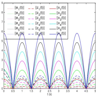
bI 32(zsI3(t)) = ( 0.14, _|zI s3(t)|61.5, −0.25, |zsI3(t)|>1.5, bI 33(zIs3(t)) = ( 0.31, |zIs3(t)|61.5, 0.25, |zIs3(t)|>1.5, dR 11(zRs1(t)) = ( −0.36, _|zR s1(t)|61.5, −0.15, _|zR s1(t)|>1.5, dR 12(zRs1(t)) = ( −0.26, _|zR s1(t)|61.5, −0.25, |zsR1(t)|>1.5, dR 13(zRs1(t)) = ( 0.24, |zsR1(t)|61.5, −0.13, |zsR1(t)|>1.5, dR 21(zsR2(t)) = ( 0.13, _|zsR2(t)|61.5, 0.25, _|zR s2(t)|>1.5, dR 22(zRs2(t)) = ( −0.25, _|zR s2(t)|61.5, −0.17, |zsR2(t)|>1.5, dR 23(zRs2(t)) = ( −0.12, |zsR2(t)|61.5, 0.23, |zsR2(t)|>1.5, dR 31(zRs3(t)) = ( −0.25, |zsR3(t)|61.5, 0.27, _|zR s3(t)|>1.5, dR 32(zsR3(t)) = ( 0.23, _|zR s3(t)|61.5, 0.11, |zsR3(t)|>1.5, dR 33(zRs3(t)) = ( −0.13, |zsR3(t)|61.5, −0.14, |zsR3(t)|>1.5, dI 11(zIs1(t)) = ( −0.16, |zsI1(t)|61.5, −0.26, _|zI s1(t)|>1.5, dI 12(zsI1(t)) = ( 0.26, _|zI s1(t)|61.5, 0.15, |zsI1(t)|>1.5, dI 13(zIs1(t)) = ( 0.21, |zsI1(t)|61.5, −0.13, |zsI1(t)|>1.5, dI 21(zsI2(t)) = ( 0.22, |zsI2(t)|61.5, 0.28, _|zI s2(t)|>1.5, dI 22(zIs2(t)) = ( −0.24, _|zI s2(t)|61.5, 0.16, _|zI s2(t)|>1.5, dI 23(zIs2(t)) = ( 0.22, |zsI2(t)|61.5, −0.11, |zsI2(t)|>1.5, dI 31(zIs3(t)) = ( −0.11, |zsI3(t)|61.5, −0.16, _|zI s3(t)|>1.5, dI 32(zIs3(t)) = ( −0.24, _|zI s3(t)|61.5, 0.11, _|zI s3(t)|>1.5, dI 33(zIs3(t)) = ( −0.34, |zsI3(t)|61.5, 0.25, |zsI3(t)|>1.5, t (s) 0 0.5 1 1.5 2 2.5 3 3.5 4 4.5 5 0 1 2 3 4 5 6 7 8 9 ||e₁(t)|| ||e₂(t)|| ||e₃(t)|| ||e₄(t)|| ||e 5(t)|| ||e 6(t)|| ||z₁(t)|| ||z₂(t)|| ||z₃(t)|| ||z₄(t)|| ||z 5(t)|| ||z 6(t)|| ||x₁(t)|| ||x₂(t)|| ||x₃(t)|| ||x₄(t)|| ||x 5(t)|| ||x 6(t)||

Fig. 1. The norms ofes(t),zs(t),xs(t), s= 1,2,_{· · ·},6.

H =         −0.6 0.2 0.1 0 0.2 0.1 0.2 −0.7 0.1 0 0.3 0.1 0.1 0.1 −0.9 0.1 0.5 0.1 0 0 0.1 −0.4 0.2 0.1 0.2 0.3 0.5 0.2 −1.4 0.2 0.1 0.1 0.1 0.1 0.2 −0.6         . Obviously, fR i (·), fiI(·), hRi (·), and hIi(·)(i = 1,2,3)

satisfy Assumption 1 with FR

i = FiI = HsR = HsI = 0.5 and lR s = l I s = η R s = η I s = 0.5. The input xs1(t) =

0.6scos(t) +i0.3scos(t), xs2(t) = 0.2scos(t) +i0.2scos(t),

xs3(t) = 0.4scos(t) + i0.5scos(t). The parameters in the

controller (7) are chosen as follows:ΥR_{= diag(0}_.₉_,₁_.₂_,₀_.₆₎_, ΥI _{= diag(0}_.₈_,₁_.₀_,₀_.₉₎_{. Take}_W 1 andW2 as follows: W1=   0 0.4 0 0.2 −0.5 0.2 0.3 0 −0.2  , W2=   −0.1 0.2 0.3 0 −0.4 0.1 0.2 0.5 −0.3  .

By using the MATLAB, it is easy to obtain thatρ= 3.7220

which satisfies the condition (8). On the basis of Theorem III.1, the system (36) is passive under controller (7). Fig. 1 shows the evolutions of error, output and input of six nodes when the system (36) is passive. Similarly, through a simple operation based on the above parameters by utilizing the MATLAB, we can obtain

λ(ΨR 1) ={−1.6951,−1.5403,−1.4313,−1.4060,−1.3738, −1.2863,₋1.2558,₋1.2236,₋1.1933,₋1.1625, −1.1547,−1.0496,−1.0448,−1.0245,−0.9988, −0.9288,₋0.9011,₋0.8297}, λ(ΨI 1) ={−1.8403,−1.5951,−1.5236,−1.4933,−1.4547, −1.3496,−1.3313,−1.3060,−1.2738,−1.2011, −1.1863,−1.0625,−1.0558,−0.8448,−0.8245,

(8)

t (s) 0 0.5 1 1.5 2 2.5 3 3.5 4 4.5 5 0 0.5 1 1.5 2 2.5 3 3.5 4 4.5 5 ||e₁(t)|| ||e₂(t)|| ||e 3(t)|| ||e 4(t)|| ||e 5(t)|| ||e 6(t)||

Fig. 2. Time evolutions ofes(t), s= 1,2,_{· · ·},6.

−0.7988,−0.7288,−0.6297},

which satisfy the condition (29). According to Theorem III.2, the system (36) achieves synchronization. Fig. 2 depicts the simulation result of synchronization.

V. CONCLUSION

This study has concerned with a type of CCVMNNs. By using certain inequalities, Lyapunov functionals as well as the design of suitable controller, a novel criterion for ensuring passivity of the considered network has been derived. Similarly, we have also carried out some discussion on the synchronization of CCVMNNs. A simulation example has been performed to confirm the correctness of our results at the end.

REFERENCES

[1] H. Lu¨, W. L. He, Q. L. Han, and C. Peng, “Fixed-time pinning-controlled synchronization for coupled delayed neural networks with discontinuous activations,” Neural Netw., vol. 116, pp. 139 - 149, August 2019. [2] A. Chandrasekar, R. Rakkiyappan, and J. Cao, “Impulsive synchronization

of Markovian jumping randomly coupled neural networks with partly unknown transition probabilities via multiple integral approach,” Neural Netw., vol. 70, pp. 27 - 38, October 2015.

[3] W. Wu and T. Chen, “Global synchronization criteria of linearly coupled neural network systems with time-varying coupling,” IEEE Trans. Neural Netw., vol. 19, pp. 319 - 332, Februrary 2008.

[4] S. R. Lin, Y. L. Huang, and S. Y. Ren, “Analysis and pinning control for passivity of coupled different dimensional neural networks,” Neurocom-puting, vol. 321, pp. 187 - 200, December 2018.

[5] S. Y. Ren, J. L. Wang, and J. G. Wu, “Generalized passivity of coupled neural networks with directed and undirected topologies,” Neurocomput-ing, vol. 314, pp. 371 - 385, November 2018.

[6] L. O. Chua, “Memristor-the missing circuit element,” IEEE Trans. Circuit Theory, vol. 18, pp. 507 - 519, September 1971.

[7] H. Shen, T. Wang, J. D. Cao, G. P. Lu, Y. D. Song, and T. W. Huang, “Non-Fragile dissipative synchronization for markovian memristive neu-ral networks: a gain-scheduled control scheme,” IEEE Trans. Neuneu-ral Netw. Learn. Syst., vol. 30, pp. 1841 - 1853, June 2019.

[8] L. M. Wang, Z. G. Zeng, M. F. Ge, and J. H. Hu, “Global stabilization analysis of inertial memristive recurrent neural networks with discrete and distributed delays,” Neural Netw., vol. 105, pp. 65 - 74, September 2018.

[9] L. M. Wang, Y. Shen, and G. D. Zhang, “Finite-time stabilization and adaptive control of memristor-based delayed neural networks,” IEEE Trans. Neural Netw. Learn. Syst., vol. 28, pp. 2648 - 2659, November 2017.

[10] Q. Xiao and Z. G. Zeng, “Lagrange stability for T-S fuzzy memristive neural networks with time-varying delays on time scales,” IEEE Trans. Fuzzy Syst., vol. 26, pp. 1091-1103, June 2018.

[11] Y. L. Huang, S. H. Qiu and S. Y. Ren, “Finite-time synchronization and passivity of coupled memristive neural networks,” Int. J. Control., doi: 10.1080/00207179.2019.1566640, January 2019.

[12] Y. V. Pershin and M. D. Ventra, “Experimental demonstration of associative memory with memristive neural networks,” Neural Netw., vol. 23, pp. 881 - 886, September 2010.

[13] S. F. Yang, Z. Y. Guo, and J. Wang, “Robust synchronization of multiple memristive neural networks with uncertain parameters via nonlinear coupling,” IEEE Trans. Syst. Man Cyber. Syst., vol. 45, pp. 1077 - 1086, July 2015.

[14] Z. Y. Guo, S. Q. Gong, S. F. Yang, and T. W. Huang, “Global exponential synchronization of multiple coupled inertial memristive neural networks with time-varying delay via nonlinear coupling,” Neural Netw., vol. 108, pp. 260 - 271, December 2018.

[15] Z. Y. Guo, S. F. Yang, and J. Wang, “Global exponential synchronization of multiple memristive neural networks with time delay via nonlinear coupling,” IEEE Trans. Neural Netw. Learn. Syst., vol. 26, pp. 1300 -1311, June 2015.

[16] Y. F. Yuan, Q. K. Song, Y. R. Liu, and F. E. Alsaadi, “Synchronization of complex-valued neural networks with mixed two additive time-varying delays,” Neurocomputing, vol. 332, pp. 149 - 158, March 2019. [17] S. Yang, J. Yu, C. Hu, and H. J. Jiang, “Quasi-projective synchronization

of fractional-order complex-valued recurrent neural networks,” Neural Netw., vol. 104, pp. 104 - 113, August 2018.

[18] Y. Kan, J. Q. Lu, J. L. Qiu, and J. G. Kurths, “Exponential synchro-nization of time-varying delayed complex-valued neural networks under hybrid impulsive controllers,” Neural Netw., vol. 114, pp. 157 - 163, June 2019.

[19] H. Zhang, X. Y. Wang, and X. H. Lin, “Synchronization of complex-valued neural network with sliding mode control,” J. Frankl. Inst., vol. 353, pp. 345 - 358, January 2016.

[20] H. M. Wang, S. K. Duan, T. W. Huang, L. D. Wang, and C. D. Li, “Exponential stability of complex-Valued memristive recurrent neural networks,” IEEE Trans. Neural Netw. Learn. Syst., vol. 28, pp. 766 -771, March 2017.

[21] W. W. Zhang, H. Zhang, J. D. Cao, Fuad E. Alsaadi, and D. Y. Chen, “Synchronization in uncertain fractional-order memristive complex-valued neural networks with multiple time delays,” Neural Netw., vol. 110, pp. 186 - 198, February 2019.

[22] R. Rakkiyappan, K. Sivaranjani, and G. Velmurugan, “Passivity and pas-sification of memristor-based complex-valued recurrent neural networks with interval timevarying delays,” Neurocomputing, vol. 144, pp. 391 -407, November 2014.

[23] X. D. Li, R. Rakkiyappan, and G. Velmurugan, “Dissipativity analysis of memristor-based complex-valued neural networks with time-varying delays,” Inf. Sci., vol. 294, pp. 645 - 665, January 2018.