A FAST ALGORITHM FOR THE NONPARAMETRIC MAXIMUM LIKELIHOOD ESTIMATE IN THE COX-GENE
MODEL
I-Shou Chang1, Chi-Chung Wen2, Yuh-Jenn Wu3 and Che-Chi Yang4 1National Health Research Institutes,
2Tamkang University, 3 Chung Yuan Christian University and 4 Lunghwa University of Science and Technology
Abstract: The Cox model with the gene effect for age at onset was introduced and studied by Li, Thompson and Wijsman (1998) and Li and Thompson (1997). This paper concerns the numerical performance of the nonparametric maximum likelihood estimate of the environmental effects and the genetic effect in this model. Based on the self-consistency equations derived from the score functions, we propose a fast iterative algorithm for the computations of the nonparametric maximum likelihood estimate and its asymptotic variance. Simulation studies conducted using these algorithms indicate that the profile likelihood-based normal approximations for the estimates are valid with reasonable sample sizes, and the bootstrap methods work well also for smaller sample sizes, and are computationally feasible.
Key words and phrases: Age at onset, bootstrap, frailty, gene effect, profile likeli-hood, self-consistency equations.
1. Introduction
Analysis of familial diseases with variable age at onset is common in hu-man genetics. Several papers have considered regression models where age at onset depends on observed individual environment effects and unobserved gene effect. See, for example, Vaupel, Manton and Stallard (1979), Meyer and Eaves (1988), Elston and George (1989), Abel and Bonney (1990), Mack, Langholz and Thomas (1990), Gauderman and Thomas (1994), Yashin and Iachine (1995), Li and Thompson (1997), etc. In particular, Li et al. (1998) and Siegmund and McKnight (1998) proposed maximum likelihood estimation of the gene effect for age at onset with semiparametric models for right censored data. These models study genetic effect at an individual level and extend classical semiparametric hazard models by the introduction of a binary frailty allowing for shared frailty within families. In order to implement this likelihood approach, Li et al. (1998) and Siegmund and McKnight (1998) studied Monte Carlo methods based on the
EM algorithm,then did some simulation studies. The model in Li et al. (1998) is called the Cox-gene model and is the main concern of the present paper.
Chang, Hsiung, Wang and Wen (2005) gave a theoretical justification of the maximum likelihood estimates in Li et al. (1998) and some of those in Siegmund and McKnight (1998). More precisely, it indicated conditions under which the parameters are identifiable and the estimate is consistent, asymptotically normal and efficient. Furthermore, it suggested that the characterization of the score functions developed for the asymptotic theory provides an alternative approach to the calculation of the nonparametric maximum likelihood estimates, hence-forth NPMLE, and that asymptotic variances can be estimated consistently using the theory of observed profile information. In this paper, we present numerical methods suggested by this theory and use them to illustrate the above likelihood methods through simulation studies.
The basis of our algorithms for the computations of the NPMLE and the asymptotic variance is a class of self-consistency equations derived from the score functions. That these are fast algorithms, as compared with the EM-algorithm implemented in Li et al. (1998) and Siegmund and McKnight (1998), is seen clearly in the simulation studies. The simulation studies in Li et al. (1998) involved one replicate only, and those in Siegmund and McKnight (1998) did not calculate variances.
To make the discussion more focused, we only consider families consisting of siblings. For this type of family, Chang et al. (2005) showed that the the-ory is valid when there are three or more siblings in each family and, in case there are observable environmental effects, it is valid even if there is only one member in each family. Our simulation studies indicate clearly that the normal approximation of the NPMLE holds with reasonable sample sizes.
To indicate that the likelihood methods do not require a fixed family size, we show by simulations that asymptotic normality seems also to hold for families with varying sizes. We note that Chang et al. (2005) assumes every family has the same number of individuals.
To take advantage of the speed of our algorithms, we also conducted boot-strap studies, and found that the bootboot-strap methods may provide better confi-dence interval when sample size is smaller and the normal approximation is not adequate.
This paper is organized as follows. Section 2 recapitulates the main results in Chang et al. (2005) and presents the self-consistency equations that lead to the algorithms presended in Section 3. Section 4 presents the simulations stud-ies, that examine the normal approximations for the NPMLE, the performance of the bootstrap methods for the Cox-gene model, and other properties of the
algorithms. Section 5 has some discussion. We give results concerning the con-vergence of the algorithms in the Appendix.
2. The Model and the Score
The notations and assumptions in this paper are consistent with those in Chang et al. (2005). In order to have a concise presentation, some of the regu-larity conditions are not stated here.
Let Tik, Cik, and Zik denote, respectively, the age at onset, the censoring time, and the covariate of theith individual in thekth family. Herei= 1, . . . , mk, k= 1, . . . , K. Let gik be the genotype of the ith individual in the kth family at a certain locus. Assume that there are two alleles at this locus and denote them
byAand a. Thus the genotype takes one of the three values, aa,aAorAA. Let
Sik =I[gik=aA or AA]denote the susceptibility type. Denote by q0 the population
allele frequency ofA.
Let Tk = (T1k, . . . , Tmkk), Ck = (C1k, . . . , Cmkk), Zk = (Z1k, . . . , Zmkk) and Sk = (S1k, . . . , Smkk). Assume that, given Zk and Sk, T1k, . . . , Tmkk, C1k, . . .,
Cmkk are conditionally independent, and for an individual having covariate z
and susceptibility type s, the hazard of disease onset at aget is
λ0(t) exp(βT0z+µ0s). (1)
Here,λ0(·) is a non-negative deterministic baseline function,β0 ∈ ℜD,Zik ∈ ℜD, andµ0 >0. Assume further that (Ck, Zk) and Skare independent, and that the distribution of (Ck, Zk) does not involve λ0(·), β0, µ0, and q0. Assume Zik is non-degenerate for everyiand k. LetXik =Tik∧Cik, the minimum ofTik and Cik, and δik=I[Tik≤Cik].
Assume that the (Tk, Ck, Zk, Sk) are independent,k= 1, . . . , K. The statis-tical problem is to estimate (Λ0, β0, µ0, q0) based on {Xk, δk, Zk|k = 1, . . . , K}, whereXk= (X1k, . . . , Xmkk),δk= (δ1k, . . . , δmkk), and Λ0(t) =
Rt
0λ0(u)du. The NPMLE (ˆΛ,β,ˆ µ,ˆ q) studied in Li et al. (1998), Siegmund and McKnightˆ (1998) and Chang et al. (2005) is the maximizer of the likelihood
LK(Λ, β, µ, q) ≡ K Y k=1 X s∈S p(s, q) mk Y i=1
[△Λ(Xik)eβTZik+µSik]δikexp[−Λ(Xik)eβTZik+µSik]
!
. (2)
Here △Λ(t) = Λ(t)−Λ(t−), Λ is a non-decreasing function with Λ(0) = 0, p(s, q) ≡ p(s1, . . . , smk, q) is the probability that the susceptibility vector takes
the value (s1, . . . , smk) when the dominant alleleAhas frequency q, andS is the
on the family structure and is calculated here under the assumptions of random mating and Mendelian segregation. To simplify the notation, we suppress the subscript k in p(s, q). For the purpose of computation, the parameter space we consider is Θc = { (Λ, β, µ, q) | Λ ∈ Lc, β ∈ B, µ ∈ U, q ∈ Q }. Here, Lc ={ Λ : [0, τ]→ [0,∞) | Λ(0) = 0, Λ(τ) ≤ c, Λ is non-decreasing and right continuous }for some τ >0 andc >0;B andU are compact subsets of ℜD and (0,∞), respectively; andQ is a closed subinterval of (0,1). The true parameters β0,µ0, andq0are assumed to be interior points ofB,U, andQ, respectively, and Λ0(τ) is assumed to be less thanc.
It follows from Theorem 4.1 and Theorem 5.1 in Chang et al. (2005) that √
K( ˆβK−β0)T,µKˆ −µ0,qKˆ −q0 T
is asymptotically normal with mean 0 and variance Σ−1, and that Σ can be estimated consistently as follows. Let
MK(β, µ, q) = 1 K Λsup∈Lc logLK(Λ, β, µ, q). (3) Then νTΣν is approximately −2MK(( ˆβ T K,µK,ˆ qK)ˆ T +γKνK)−MK(( ˆβKT,µK,ˆ qK)ˆ T) γK2 (4)
for every sequence νK, in ℜD+2, converging in probability to ν, and for every sequence γK satisfying (√KγK)−1 =Op(1) and γK =op(1).
We now introduce notations so that we can state several equations that are useful in proposing the algorithms. These equations are derived from the score functions. Let fk(Λ, β, µ, q, s) =p(s, q) mk Y i=1 eµsiδikexp[−Λ(X ik)eβ TZ ik+µsi] ! , WK(Λ, β, µ, q;u) = 1 K K X k=1 mk X i=1 P sfk(Λ, β, µ, q, s)eβ TZ ik+µsi P sfk(Λ, β, µ, q, s) I(0,Xik](u), GK(u) = 1 K K X k=1 mk X i=1 I[Tik,∞)(u∧Cik), bk(Λ, β, µ, q, s) =fk(Λ, β, µ, q, s)/p(s, q). Knowing that ∂
∂qp(s, q) is a polynomial inq, we delete the monomials in
∂ ∂qp(s, q) having negative coefficients and denote the resulting polynomial byp′+(s, q). Let p′−(s, q) =p
′
+(s, q)− ∂q∂p(s, q). Let e T
1 = (1,0,0, . . . ,0), eT2 = (0,1,0, . . . ,0), . . ., eTD = (0,0,0, . . . ,1). The NPMLE (ˆΛ,β,ˆ µ,ˆ q) satisfies the following.ˆ
Proposition 1. (i) ˆ Λ(t) = Z t 0 1 WK(ˆΛ,β,ˆ µ,ˆ qˆ;u)dGK(u); (5) (ii) ˆ βTej= log K P k=1 mk P i=1 δikeTjZik K P k=1 mPk i=1 P sfk(ˆΛ,β,ˆˆµ,q,s)(eˆ TjZikΛ(Xˆ ik)exp( ˆβT(Zik−ej)+ˆµsi)) P sfk(ˆΛ,β,ˆµ,ˆˆq,s) forj = 1, . . . , D; (6) (iii) ˆ µ= log K P k=1 mk P i=1 P sfk(ˆΛ,β,ˆˆµ,ˆq,s)(δiksi) P sfk(ˆΛ,β,ˆµ,ˆˆq,s) K P k=1 mk P i=1 P sfk(ˆΛ,β,ˆˆµ,ˆq,s)(siΛ(Xˆ ik)exp( ˆβZik+ˆµ(si−1))) P sfk(ˆΛ,β,ˆµ,ˆˆq,s) ; (7) (iv) ˆ q= K P k=1 P sˆqp ′ +(s,ˆq)bk(ˆΛ,β,ˆµ,ˆˆq,s) P sfk(ˆΛ,β,ˆˆµ,ˆq,s) K P k=1 P sp ′ −(s,q)bˆ k(ˆΛ,β,ˆµ,ˆq,s)ˆ P sfk(ˆΛ,β,ˆˆµ,ˆq,s) . (8)
Remarks. We note that part (i) in Proposition 1 is just the first part of Lemma 2.1 in Chang et al. (2005), and (ii), (iii), and (iv) are derived, respectively, from the score functions (2.4), (2.5), and (2.6) there. Although the proof of Proposition 1 is straightforward and hence omitted, we would like to point out that it is the basis of the following algorithms, the main ideas of which are explained in the Appendix. In fact, part (ii), (iii), and (iv) of Proposition 1 are motivated by Proposition 3 in the Appendix. Specifically, suppose the score function is represented as the derivative η′
1 of a function η1, with η1′(α0) = 0 and α0 >0. If η′
1 = η2 −η3 for two positive functions η2 and η3, α1 is close to α0, and αJ+1 = αJ[η2(αJ)/η3(αJ)], then αJ converges to α0 under certain regularity conditions. With suitably chosen η2 andη3, we get (ii), (iii), and (iv). Consider (iv), for example. We set
η2= K X k=1 P sqpˆ ′ +(s,q)bk(ˆˆ Λ,β,ˆ µ,ˆ q, s)ˆ P sfk(ˆΛ,β,ˆ µ,ˆ q, s)ˆ , η3 = K X k=1 P sp ′ −(s,q)bk(ˆˆ Λ,β,ˆ µ,ˆ q, s)ˆ P sfk(ˆΛ,β,ˆ µ,ˆ q, s)ˆ . Thenη2−η3is the score function and step (5) in Algorithm 3.1 is an implementa-tion ofαJ+1=αJ[η2(αJ)/η3(αJ)]. We note that although the Newton-Ralphson
method is also an iterative procedure and applicable here, our (unreported) sim-ulation studies indicate that it is very slow.
3. Algorithm
Let L(ˆΛ,β,ˆ µ,ˆ q)(t),ˆ Bj(ˆΛ,β,ˆ µ,ˆ q),ˆ M(ˆΛ,β,ˆ µ,ˆ q), andˆ Q(ˆΛ,β,ˆ µ,ˆ q) denote,ˆ respectively, the right hand sides of (5), (6), (7) and (8). Let B(ˆΛ,β,ˆ µ,ˆ q) =ˆ (B1(ˆΛ,β,ˆ µ, ˆˆ q),. . . ,BD(ˆΛ,β,ˆ µ,ˆ q))ˆ T.
3.1. Algorithm for Estimating ˆΛ, ˆβ, ˆµ, ˆq, and ˆΣ
(1) Choose starting values Λ1,β1,µ1, and q1. (2) Set J = 1. (3) βJ+1 =B(ΛJ, βJ, µJ, qJ). (4) µJ+1=M(ΛJ, βJ+1, µJ, qJ). (5) qJ+1 =Q(ΛJ, βJ+1, µJ+1, qJ). (6) ΛJ+1(t) =L(ΛJ, βJ+1, µJ+1, qJ+1)(t). (7) J =J + 1.
(8) Repeat (3) for a suitable number N of iterations once there is evidence of convergence.
(9) The estimates of Λ, β,µ,q are given by ˆΛ = ΛN, ˆβ=βN, ˆµ=µN, ˆq =qN, respectively.
(10) Set γK = 1/ √
K. (11) The (i, j)-entry of ˆΣ is
−hMK(( ˆβT,µ,ˆ q)ˆT +γKei+γKej)−MK(( ˆβT,µ,ˆ q)ˆT +γKei)
−MK(( ˆβT,µ,ˆ q)ˆT+γKej)+MK(( ˆβT,µ,ˆ q)ˆT)i.γK2.
3.2. Algorithm for Computing MK(β, µ, q)
(1) Choose a starting value Λ1, set L1=logLK(Λ1, β, µ, q). (2) Set J = 1.
(3) ΛJ+1(t) =L(ΛJ, β, µ, q)(t), set LJ+1 =logLK(ΛJ+1, β, µ, q). (4) J =J + 1.
(5) Repeat (3) for a suitable number N of iterations once there is evidence of convergence.
(6) MK(β, µ, q) = LN/K.
4. Simulation Studies
The purpose of this section is to assess the numerical performance of the NPMLE computed using the algorithms in Section 3. There are four parts in this section. The first part examines the normal approximation claimed in
Chang et al. (2005), the second part studies the bootstrap methods, the third part gives some idea of the dependence of the estimates on the starting values used in the algorithms, and the fourth part remarks on the computations needed for large pedigrees.
All the data are generated according to (1) withR0tλ0(s)ds= log(100/(100− t)), for t ∈ [0,100), and several different values of β0, µ0, and q0; the censoring variable is uniform(0,100); and P(Zik = 0) =P(Zik = 1) = 1/2. Except for the studies in Table 2, the number of iterations in using Algorithm 3.1 is set at 100, and that for Algorithm 3.2 is 10. In Table 2, we consider bootstrap coverage and the number of iterations in using Algorithm 3.1 is set at 50.
4.1. Normal Approximation
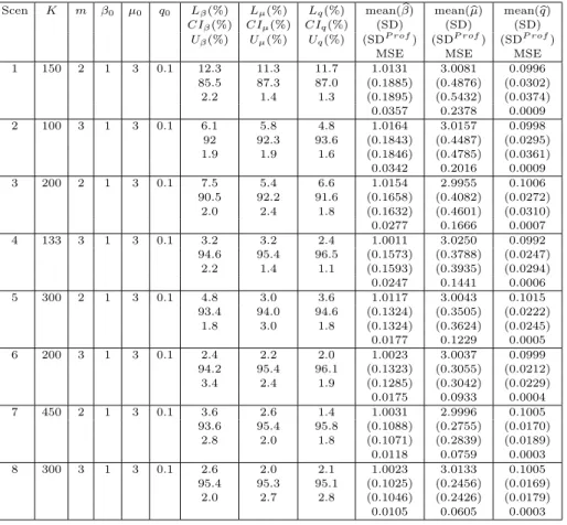
Our simulation studies indicate that the normal approximations for β,b µ,b and qbare generally quite satisfactory. They also suggest that a relatively larger sample size is needed whenq0 is near 0 orµ0is small, and a much smaller sample size is needed in case there are more siblings in each family. Among other things, Table 1A seems to suggest that if the total number of individuals is fixed, studies having larger family size tend to provide better estimates in terms of mean-squared error and confidence interval coverage. In fact, the purpose of Table 1A is to demonstrate this phenomenon.
Each study in this subsection consists of 1,000 random samples of different sample sizes. For each sample, we first use the algorithms in Section 3 to compute
b
β,µ,b q, andb Σ, and then use the asymptotic normality to get a 0.95 confidenceb
interval. The number of these 1,000 samples for which the true parameter falls in its 0.95 confidence interval is recorded; these numbers are then used to get the 95% confidence interval coverage, which is expressed in percentiles in the seventh, eighth and ninth columns of Table 1. We useCIβ, CIµ,andCIq to indicate the columns for β,µ, and q, respectively. The percentages of the samples for which the true parameter β0, µ0,and q0 falls below (above) its 0.95 confidence interval are also contained in these columns and denoted byLβ(Uβ), Lµ(Uµ),andLq(Uq) respectively. Each row in Table 1 represents the results for one simulation study scenario. We use Scen-a to denote the study presented in the ath row in Table 1. Here a= 1, . . . ,15.
Each family in our studies consists of siblings. The second and third columns are, respectively, the sample sizeK and the numbermof siblings in each family. The next three columns contain, respectively, the true parameter values β0, µ0 andq0used in the data generation. The tenth, eleventh, and twelfth columns give the sample mean, sample standard deviation (SD), averaged standard deviation computed by profile likelihood (SDP rof) of the 1,000 estimates, and sample mean-squared error (MSE) forβ0,µ0, and q0, respectively.
We note that the family sizes in the last two rows in Table 1B are random, 2 + Bi(4, 0.3) where Bi(4, 0.3) is the binomial random variable with parameters 4 and 0.3, implying that the average family size is 3.2.
The starting values used in the algorithms for each study in this section are Λ1(t) =t/80,β1= 0.9,µ1 = 3.55, andq1 = 0.16.
In some of the studies,µ0is equal to 4.6052. We note that exp(4.6052) = 100, which is the genetic relative risk used in Siegmund and McKnight (1998), and studied in Mack et al. (1990).
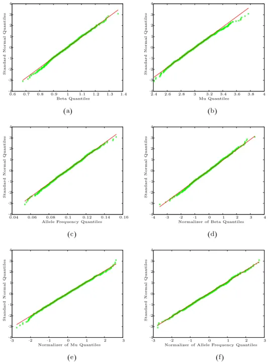
Figure 1 presents the Q-Q plots for the experiment in Scen-14. Figure 1 strongly suggests an asymptotic normality theory for family with varying sizes, which was not discussed in Chang et al. (2005).
Table 1. 0.95 confidence interval coverage, expressed in percentile, sample mean, sample standard deviation (SD), averaged standard deviation
com-puted by profile likelihood (SDP rof), and sample mean-squared error (MSE),
for 15 simulation study scenarios.
Scen K m β0 µ0 q0 Lβ(%) Lµ(%) Lq(%) mean(βb) mean(µb) mean(qb)
CIβ(%) CIµ(%) CIq(%) (SD) (SD) (SD)
Uβ(%) Uµ(%) Uq(%) (SDP rof) (SDP rof) (SDP rof)
MSE MSE MSE
1 150 2 1 3 0.1 12.3 11.3 11.7 1.0131 3.0081 0.0996 85.5 87.3 87.0 (0.1885) (0.4876) (0.0302) 2.2 1.4 1.3 (0.1895) (0.5432) (0.0374) 0.0357 0.2378 0.0009 2 100 3 1 3 0.1 6.1 5.8 4.8 1.0164 3.0157 0.0998 92 92.3 93.6 (0.1843) (0.4487) (0.0295) 1.9 1.9 1.6 (0.1846) (0.4785) (0.0361) 0.0342 0.2016 0.0009 3 200 2 1 3 0.1 7.5 5.4 6.6 1.0154 2.9955 0.1006 90.5 92.2 91.6 (0.1658) (0.4082) (0.0272) 2.0 2.4 1.8 (0.1632) (0.4601) (0.0310) 0.0277 0.1666 0.0007 4 133 3 1 3 0.1 3.2 3.2 2.4 1.0011 3.0250 0.0992 94.6 95.4 96.5 (0.1573) (0.3788) (0.0247) 2.2 1.4 1.1 (0.1593) (0.3935) (0.0294) 0.0247 0.1441 0.0006 5 300 2 1 3 0.1 4.8 3.0 3.6 1.0117 3.0043 0.1015 93.4 94.0 94.6 (0.1324) (0.3505) (0.0222) 1.8 3.0 1.8 (0.1324) (0.3624) (0.0245) 0.0177 0.1229 0.0005 6 200 3 1 3 0.1 2.4 2.2 2.0 1.0023 3.0037 0.0999 94.2 95.4 96.1 (0.1323) (0.3055) (0.0212) 3.4 2.4 1.9 (0.1285) (0.3042) (0.0229) 0.0175 0.0933 0.0004 7 450 2 1 3 0.1 3.6 2.6 1.4 1.0031 2.9996 0.1005 93.6 95.4 95.8 (0.1088) (0.2755) (0.0170) 2.8 2.0 1.8 (0.1071) (0.2839) (0.0189) 0.0118 0.0759 0.0003 8 300 3 1 3 0.1 2.6 2.0 2.1 1.0023 3.0133 0.1005 95.4 95.3 95.1 (0.1025) (0.2456) (0.0169) 2.0 2.7 2.8 (0.1046) (0.2426) (0.0179) 0.0105 0.0605 0.0003
Table 1B.
Scen K m β0 µ0 q0 Lβ(%) Lµ(%) Lq(%) mean(βb) mean(µb) mean(bq)
CIβ(%) CIµ(%) CIq(%) (SD) (SD) (SD)
Uβ(%) Uµ(%) Uq(%) (SDP rof) (SDP rof) (SDP rof)
MSE MSE MSE
9 1400 1 1 3 0.1 3.1 16.3 6 1.0076 3.0184 0.1018 94 74.7 92.4 (0.0897) (0.3025) (0.0187) 2.9 9 1.6 (0.0886) (0.2713) (0.0182) 0.0081 0.0918 0.0004 10 2400 1 1 3 0.1 2.8 12.5 4.5 1.0031 3.0118 0.1008 94.4 78.5 93.2 (0.0678) (0.2287) (0.0133) 2.8 9 2.3 (0.0676) (0.2319) (0.0141) 0.0046 0.0524 0.0002 11 300 3 1 4.6052 0.05 2.1 4 0.7 1.0077 4.6319 0.0495 96.1 93.2 98.5 (0.0902) (0.3830) (0.0087) 1.8 2.8 0.8 (0.0950) (0.3649) (0.0107) 0.0082 0.1474 0.0001 12 500 3 1 4.6052 0.01 2.3 3.4 1.1 1.0082 4.5278 0.0105 94.9 90.3 97.5 (0.0732) (0.6233) (0.0042) 2.8 6.3 1.4 (0.0714) (0.4115) (0.0065) 0.0054 0.3945 0.0000 13 700 3 1 4.6052 0.01 2.4 3.2 1.1 1.0009 4.5955 0.0103 95.6 92.5 98.7 (0.0571) (0.4565) (0.0037) 2.0 4.3 0.2 (0.0602) (0.3340) (0.0050) 0.0033 0.2085 0.0000 14 300 3.2 1 3 0.1 2.5 2.4 1.6 0.9991 3.0033 0.0994 95.1 95.9 96 (0.1032) (0.2210) (0.0159) 2.4 1.7 2.4 (0.1004) (0.2257) (0.0171) 0.0107 0.0489 0.0003 15 400 3.2 1 4.6052 0.01 2.6 3.3 2.3 1.0024 4.5421 0.0107 95.2 90.9 96.5 (0.0770) (0.6650) (0.0051) 2.2 5.8 1.2 (0.0770) (0.4186) (0.0071) 0.0059 0.4462 0.0000 4.2. Bootstrap
These studies confirm the expected benefits of the bootstrap (Efron and Tibshirani (1993)): when the normal approximation is satisfactory, bootstrap methods seem to perform as well; when the normal approximation fails, bootstrap methods may still offer reasonable solutions.
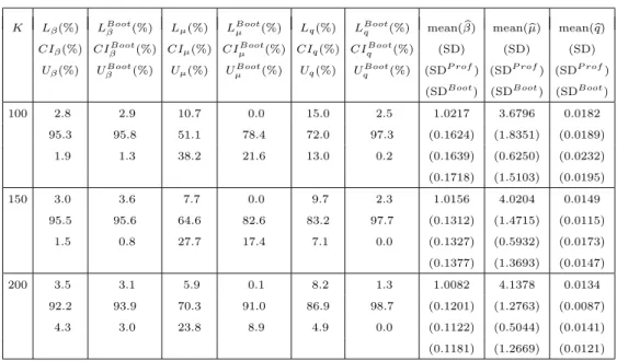
The bootstrap results are reported in Table 2. In Table 2, the first column is the sample size; the second, fourth, and sixth columns report, respectively, the same statistics reported in the seventh, eighth, and ninth columns in Table 1; the third, fifth, and seventh columns are, respectively, the bootstrap counterparts of the second, fourth, and sixth columns; the eighth, ninth, and tenth columns, re-spectively, report the same statistics in the tenth, eleventh, and twelfth columns in Table 1, except for the replacement of MSE by SDBoot, which is the aver-aged standard deviation calculated by the bootstrap method. We note that the bootstrap sample size is 1,000 and the coverage is based on 200 replicates.
It is seen from Table 2 that normal approximation and bootstrap are compa-rable and satisfactory for β,normal approximation is less satisfactory than the bootstrap for µ and q; in particular, SDBoot is much closer to SD for µ than is SDP rof.
( ) ( ) -- - - ( ) ( ) - - -- - ( ) ( ) 0.6 0.7 0.8 0.9 1.1 1.2 1.3 1.4 2.4 2.6 2.8 3.2 3.4 3.6 3.8 a b c d e f 0 0 0 0 0 0 0 0 0 1 1 1 1 1 1 1 1 1 1 1 1 1 1 1 1 1 1 1 2 2 2 2 2 2 2 2 2 2 2 2 2 2 2 2 2 2 3 3 3 3 3 3 3 3 3 3 3 3 3 3 3 3 3 3 3 4 4 4 4 4 4 4 4 4 4 4 4 4 4 4 Mu Quantiles S t a n d a r d N o r m a l Q u a n t il e s Beta Quantiles S t a n d a r d N o r m a l Q u a n t il e s
Allele Frequency Quantiles
S t a n d a r d N o r m a l Q u a n t il e s
Normalizer of Beta Quantiles
S t a n d a r d N o r m a l Q u a n t il e s Normalizer of Mu Quantiles S t a n d a r d N o r m a l Q u a n t il e s
Normalizer of Allele Frequency Quantiles
S t a n d a r d N o r m a l Q u a n t il e s 0.04 0.06 0.08 0.1 0.12 0.14 0.16
Figure 1. Q-Q plots for the study in Scen-14. (a) Q-Q plot of ˆβvs. standard
normal. (b) Q-Q plot of ˆµ vs. standard normal. (c) Q-Q plot of ˆq vs.
standard normal. (d) Q-Q plot of normalizer of ˆβ vs. standard normal. (e)
Q-Q plot of normalizer of ˆµvs. standard normal. (f) Q-Q plot of normalizer
Table 2. Comparison of normal approximation and the bootstrap methods
form= 3, β0= 1, µ0= 4.6052, q0= 0.01.
K Lβ(%) LBootβ (%) Lµ(%) LBootµ (%) Lq(%) LBootq (%) mean(βb) mean(bµ) mean(bq)
CIβ(%) CIβBoot(%) CIµ(%) CIµBoot(%) CIq(%) CIBootq (%) (SD) (SD) (SD)
Uβ(%) UβBoot(%) Uµ(%) UµBoot(%) Uq(%) UqBoot(%) (SDP rof) (SDP rof) (SDP rof)
(SDBoot) (SDBoot) (SDBoot)
100 2.8 2.9 10.7 0.0 15.0 2.5 1.0217 3.6796 0.0182 95.3 95.8 51.1 78.4 72.0 97.3 (0.1624) (1.8351) (0.0189) 1.9 1.3 38.2 21.6 13.0 0.2 (0.1639) (0.6250) (0.0232) (0.1718) (1.5103) (0.0195) 150 3.0 3.6 7.7 0.0 9.7 2.3 1.0156 4.0204 0.0149 95.5 95.6 64.6 82.6 83.2 97.7 (0.1312) (1.4715) (0.0115) 1.5 0.8 27.7 17.4 7.1 0.0 (0.1327) (0.5932) (0.0173) (0.1377) (1.3693) (0.0147) 200 3.5 3.1 5.9 0.1 8.2 1.3 1.0082 4.1378 0.0134 92.2 93.9 70.3 91.0 86.9 98.7 (0.1201) (1.2763) (0.0087) 4.3 3.0 23.8 8.9 4.9 0.0 (0.1122) (0.5044) (0.0141) (0.1181) (1.2669) (0.0121) 4.3. Starting Values
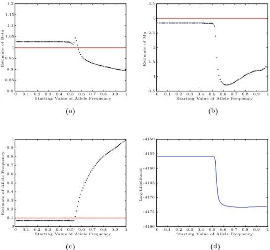
Since the NPMLE and the algorithms we use are local in nature, the esti-mates may depend on the starting valuesβ1,µ1, andq1. Based on our simulation studies, it seems that the dependence on the starting values is not a serious prob-lem forβ and µ, and even forq we need only set the starting value less than 0.5. Using data of Scen-8, we report the results regarding the dependence on q1. With the starting values for Λ1,β1, andµ1 being fixed, we calculateβ,b bµ, qbfor q1 = 0.01,0.02, . . . ,0.99. Plots for (q1,β), (q1,b µ), (q1,b q), and a plot forb q1 vs. log-likelihood are presented in Figure 2.
4.4. Remarks on Pedigree Size
Examining (2) closely, we know that the numerical performance of our method depends on pedigree structure only through the number of individuals in the pedi-gree and the susceptibility probability p(s, q). Becausep(s, q) is a polynomial in q,the computation for sibship data is no easier than that for other pedigree data with the same number of individuals in one pedigree. With this understanding, we consider only sibship data in the following.
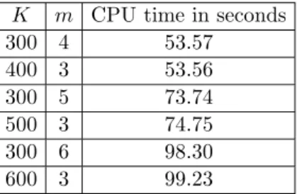
We report in Table 3 the average computing time needed for analyzing one set of simulated sibship data under the parameter values β0 = 1, µ0 = 3, q0 = 0.1
and Λ0(t) = log(100/(100−t)), and using the algorithms in Section 3. More precisely, for each replicate, we calculate the NPMLE and their asymptotical variances; we report the average of the computing times based on ten replicates. It seems clear from Table 3 that the computing time needed depends mainly on the total number of individuals in the study, not on the size of the pedigree. This, together with Table 1A, indicates that it is more desirable to conduct studies having relatively larger pedigree when the total number of individuals in the study is fixed. We do not recommend a study of only one pedigree, because this offers little possibility to study the variance of the estimates.
( ) ( )
( ) ( )
a b
c d
Starting Value of Allele Frequency
E s t im a t e o f B e t a
Starting Value of Allele Frequency
E s t im a t e o f M u
Starting Value of Allele Frequency
E s t im a t e o f A ll e le F r e q u e n c y
Starting Value of Allele Frequency
L o g -L ik e li h o o d 0 0 0 0 0 0.1 0.1 0.1 0.1 0.1 0.2 0.2 0.2 0.2 0.2 0.3 0.3 0.3 0.3 0.3 0.4 0.4 0.4 0.4 0.4 0.5 0.5 0.5 0.5 0.5 0.5 0.6 0.6 0.6 0.6 0.6 0.7 0.7 0.7 0.7 0.7 0.8 0.8 0.8 0.8 0.8 0.8 0.85 0.9 0.9 0.9 0.9 0.9 0.9 0.95 1 1 1 1 1 1 1 1.05 1.1 1.15 1.2 1.5 2 2.5 3 3.5 -4180 -4175 -4170 -4165 -4160 -4155 -4150
Figure 2. Starting value study in Scen-8. Dotted lines are the estimates;
solid lines are true parameters. (a) Plot ofq1 vs. ˆβ. (b) Plot ofq1 vs. ˆµ.
Table 3. Computing time needed for sibship data whenβ0= 1, µ0= 3, q0=
0.1,and Λ0(t) = log(100/(100−t)). Here K is the number of families and
mis the number of individuals in one family.
K m CPU time in seconds
300 4 53.57 400 3 53.56 300 5 73.74 500 3 74.75 300 6 98.30 600 3 99.23 5. Discussion
We have presented a fast algorithm for computing the NPMLE through the Cox-gene model, and used it to study the likelihood theory and the bootstrap methods for the Cox-gene model through simulation studies. Our simulation studies indicate that the normal approximations of the NPMLE work well with reasonable sample sizes. In case of smaller sample sizes for which normal ap-proximation does not work well, we find that bootstrap methods provide a useful alternative.
The algorithms we use in this paper are based on the self-consistency equa-tions derived from the score funcequa-tions. We studied several other algorithms based on the score functions and found that the one in Section 3 is the best in terms of both accuracy and speed. In particular, the algorithms that replaceii),iii), and iv) in Proposition 1 by Newton-Ralphson methods do not perform comparably. In fact, among the computation procedures we studied, the one in the Section 3 is the only one that makes variance estimation and bootstrap methods feasible. The software, prepared with Matlab, is available from the author upon request. We have also prepared software for nuclear families consisting of parents and children.
Although this method seems satisfactory for the Cox-gene model of Li et al. (1998), we understand this work represents only a initial study toward the understanding of the mechanisms of genetic diseases. Serious efforts are needed to take into account multiple genes and environmental factors.
Acknowledgements
We are grateful to Professor Naisyin Wang and two referees for comments that led to improvement of the paper. This work is partially supported by NSC Grant 93-3112-B-400-007-Y.
Appendix
In this Appendix, we provide some heuristic ideas concerning the convergence of Algorithm 3.1 and 3.2. We do not present a rigorous and complete statement, as this is laborious. We assumemk =m for everyk to ease the presentation.
Proposition 2. For given (Λ1, β, µ, q) in its domain, let ΛJ+1(t) =
Z t 0
1
WK(ΛJ, β, µ, q;u)dGK(u)
for J = 1,2, . . ., and t∈ [0, τ]. Then there exists Ω1 with P(Ω1) = 1 such that for every ω in Ω1, there exists a constant K(ω) such that for everyK > K(ω), ΛJ(·) has a convergent subsequence, and the limit ˜Λ of any of its convergent subsequences satisfies ˜ Λ(t) = Z t 0 1 WK(˜Λ, β, µ, q;u) dGK(u). (A.1)
Proof. It follows from the definition ofWK that there exists a constant c2>0 such that WK(Λ, β, µ, q;u)≥ c2 K K X k=1 m X i=1 1(0,Xik](u)
for every K and for every (Λ, β, µ, q, u) in its domain. Hence, using the Law of Large Numbers, we getW(Λ, β, µ, q;u)≥c2
m P i=1
P(Xi1 ≥τ),whereW is the limit
of WK. This indicates that
Z τ 0
1
W(Λ, β, µ, q;u)dG(u)<∞, (A.2) for every (Λ, β, µ, q) in its domain. Using (A.2) and Lemma 3.3 in Chang et al. (2005), we know that there exists a constantc3 such that
lim K→∞ Z τ 0 1 WK(Λ, β, µ, q;u)dGK(u)< c3, (A.3)
for every (Λ, β, µ, q) in its domain. It follows from (A.3) that there exists Ω1 withP(Ω1) = 1 such that for every ω in Ω1, there is a constantK(ω) such that for everyK > K(ω),
Z τ 0
1
WK(Λ, β, µ, q;u)dGK(u)< c3.
Thus we know from Helly’s Lemma that ΛJ(·) has a convergent subsequence, and hence, (A.1) holds. This completes the proof.
Note that the convergence of Algorithm 3.2 follows from Proposition 2. Al-though Proposition 2 does not by any means imply the convergence of Algorithm 3.1, it together with the following Proposition 3 does provide relevant informa-tion. We note that there are extensions to Proposition 3, and they may also be useful in other places.
Proposition 3. Letη1 : (a, b)→ ℜbe a function possessing bounded continuous second derivative. Letα0 >0 be an isolated local maximum ofη1andη′′1(α0)<0. Letη2 andη3 be two positive and continuously differentiable functions satisfying
η1′ = η2 −η3. Then there exist constants ε > 0 and n0 ≥ 0, such that if
|α1−α0|< ε andαJ+1=αJ[(η2(αJ) +n0)/(η3(αJ) +n0)] for J = 1,2, . . ., then αJ converges toα0.
Remarks. The idea behind Proposition 3 is simple and goes as follows. If
0 < αJ < α0, then we would like to have αJ+1 > αJ. If αJ is in a suitable
neighborhood of α0 and 0 < αJ < α0,then η2(αJ)−η3(αJ) =η ′
1(αJ) >0, and henceαJ+1> αJ.Similar comments can be made for the case αJ > α0.
Proof. Let gn(x) = [(η2(x) +n)/(η3(x) +n)]. Using gn′(α0) = (η2′(α0) − η′
3(α0))/(η3(α0)+n)<0, we letn0>0 satisfygn0′ (α0)≥(2/3)·[(−c−1)/(α0+1)] for some 0< c < 1. Let 0 < ε <1 satisfy α0 > ε, [α0−ε, α0+ε]⊂(a, b), and |g′
n0(x)−g′n0(α0)|<(1/2)|gn0′ (α0)|for everyx in [α0−ε, α0+ε]. Then 1 2g ′ n0(α0)> g′n0(x)> 3 2g ′ n0(α0)≥ − c−1 α0+ε (A.4) for everyx in [α0−ε, α0+ε].
Using the equation [(αJ+1)/(αJ)]−1 = gn0(αJ)−gn0(α0) and the Mean-Value Theorem, we have
αJ+1−α0 = (αJ −α0)(1 +gn0′ (αJ)αJe ) (A.5) for someαJe lying betweenαJ and α0.
Using (A.4), we haveg′
n0(αe1)α1≥[(−c−1)/(α0+ε)]α1 >−c−1, and hence, 1+gn0′ (α1)α1e ≥ −c >−1. Using (A.4) again, we have 1+g′n0(α1e )α1 ≤1+c1α1≤ 1 +c1(α0−ε) < 1, where 0> c1 = max
x∈[α0−ε,α0+ε]g
′
n0(x). These, combined with (A.5), imply that |α2 −α0| < c2|α1 −α0| for some 0 < c2 < 1. Doing these recursively, completes the proof.
References
Abel, L. and Bonney, G. E. (1990). A time-dependent logistic hazard function for modelling variable age of onset in analysis of familial diseases. Genetic Epidemiology7, 391-407.
Chang, I. S., Hsiung, C. A., Wang, M. C. and Wen, C. C. (2005). An asymptotic theory for the nonparametric maximum likelihood estimator in the Cox-gene model. Bernoulli 11,
863-892.
Efron, B. and Tibshirani, R. J. (1993).An Introduction to the Bootstrap.Chapman & Hall, New York.
Elston, R. C. and George, V. T. (1989). Age of onset, age at examination, and other covariates in the analysis of family data.Genetic Epidemiology6, 217-220.
Gauderman, W. J. and Thomas, D. (1994). Censored survival models for genetic epidemiology: A Gibbs sampling approach.Genetic Epidemiology11, 171-188.
Li, H. and Thompson, E. A. (1997). Semiparametric estimation of major gene and family-specific random effects for age of onset. Biometrics53, 282-293.
Li, H., Thompson, E. A. and Wijsman, E. M. (1998). Semiparametric estimation of major gene effects for age of onset.Genetic Epidemiology15, 279-298.
Mack, W., Langholz B. and Thomas, D. C. (1990). Survival models for familial aggregation of cancer.Environmental Health Perspectives 87, 27-35.
Meyer, J. M. and Eaves, L. J. (1988). Estimating genetic parameters of survival distributions: A multifactorial model.Genetic Epidemiology5, 265-275.
Siegmund, K. and McKnight, B. (1998). Modeling hazard functions in families. Genetic Epi-demiology15, 147-171.
Vaupel, J. W., Manton, K. G. and Stallard, E. (1979). The impact of heterogeneity in individual frailty and the dynamics of mortality.Demography 16, 439-454.
Yashin, A. I. and Iachine, I. A. (1995). Genetic analysis of durations: Correlated frailty model applied to survival of Danish twins.Genetic Epidemiology12, 529-538.
Institute of Cancer Research and Div. of Biostatistics and Bioinformatics, National Health Research Institutes, 35, Keyan Road, Zhunan Town, Miaoli County 350, Taiwan.
E-mail: [email protected]
Department of Mathematics, Tamkang University, 151 Ying-chuan Road Tamsui, Taipei County 251, Taiwan.
E-mail: [email protected]
Department of Applied Mathematics, Chung Yuan Christian University, 200, Chung Pei Rd., Chung Li 320, Taiwan.
E-mail: [email protected]
Department of Information Management, Lunghwa University of Science and Technology, 300, Sec.1, Wanshou Rd., Guishan, Taoyuan 333, Taiwan.
E-mail: [email protected]