CHAPTER 2
LAND COVER CLASSIFICATION AND MAPPING
Introduction
Mapping natural land cover requires a higher level of effort than the development of data for animal species, agency ownership, or land management, yet it is no more important for gap analysis than any other data layer. Generally, the mapping of land cover is done by adopting or developing a land cover classification system, delineating areas of relative homogeneity (basic cartographic "objects"), then labeling these areas using categories defined by the classification system. More detailed attributes of the individual areas are added as more information becomes available, and a process of validating both spatial pattern and labels is applied for editing and revising the map. This is done in an iterative fashion, with the results from one step causing re-evaluation of results from another step. Finally, an assessment of the overall accuracy of the data is conducted. The final assessment of accuracy will show where improvements should be made in the next update (Stoms et al.1994).
In its "coarse filter" approach to conservation biology (e.g., Jenkins 1985, Noss 1987), gap analysis relies on maps of dominant natural land cover types as the most fundamental spatial component of the analysis (Scott et al. 1993) for terrestrial environments. For the purposes of GAP, most of the land surface of interest (natural) can be characterized by its dominant vegetation.
Vegetation patterns are an integrated reflection of the physical and chemical factors that shape the environment of a given land area (Whittaker 1965). They also are determinants for overall biological diversity patterns (Franklin 1993, Levin 1981, Noss 1990), and they can be used as a currency for habitat types in conservation evaluations (Specht 1975, Austin 1991). As such, dominant vegetation types need to be recognized over their entire ranges of distribution (Bourgeron et al. 1994) for beta-scale analysis (sensu Whittaker 1960, 1977). These patterns cannot be acceptably mapped from any single source of remotely sensed imagery, therefore, ancillary data, previous maps, and field surveys are used. The central concept is that the
physiognomic and floristic characteristics of vegetation (and, in the absence of vegetation, other physical structures) across the land surface can be used to define biologically meaningful biogeographic patterns. There may be considerable variation in the floristics of subcanopy vegetation layers (community association) that are not resolved when mapping at the level of dominant canopy vegetation types (alliance), and there is a need to address this part of the diversity of nature. As information accumulates from field studies on patterns of variation in understory layers, it can be attributed to the mapped units of alliances.
Land Cover Classification
Land cover classifications must rely on specified attributes, such as the structural features of plants, their floristic composition, or environmental conditions, to consistently differentiate categories (Kuchler and Zonneveld 1988). The criteria for a land cover classification system for
• an ability to distinguish areas of different actual dominant vegetation;
• a utility for modeling animal species habitats;
• a suitability for use within and among biogeographic regions;
• an applicability to Landsat Thematic Mapper (TM) imagery for both rendering a base map and from which to extract basic patterns (GAP relies on a wide array of information sources, TM offers a convenient meso-scale base map in addition to being one source of actual land cover information);
• a framework that can interface with classification systems used by other organizations and nations to the greatest extent possible; and
• a capability to fit, both categorically and spatially, with classifications of other themes such as agricultural and built environments.
For GAP, the system that fits best is referred to as the National Vegetation Classification System (NVCS) (FGDC 1997). The origin of this system was referred to as the UNESCO/TNC system (Lins and Kleckner 1996) because it is based on the structural characteristics of vegetation derived by Mueller-Dombois and Ellenberg (1974), adopted by the United Nations Educational, Scientific, and Cultural Organization (UNESCO 1973) and later modified for application to the United States by Driscoll et al. (1983, 1984). The Nature Conservancy and the Natural Heritage Network (Grossman et al. 1994) have been improving upon this system in recent years with partial funding supplied by GAP. The basic assumptions and definitions for this system have been described by Jennings (1993).
Using the National Vegetation Classification System, an alliance list was developed for the State of Nebraska. After consulations with experts and preliminary image classifications, it was determined that mapping to an alliance level with Landsat TM imagery would prove to be problematic, if not impossible, for those vegetation alliances that depend upon understory vegetation descriptions (e.g., forests and woodlands) as well as those that typically occur as small patches (e.g.,wetlands). Grouping alliances based on the NVCS hierarchical system developed a modified classification system. Most grasslands were mapped at the alliance level; whereas, wetland and woodland classes were grouped into broader classes. A final mappable land cover / alliance relationship (Table 2.1) was based upon a report from the Association for Biodiversity Information (2001) with expert guidance from ABI (S. Menard, personal
communication 3/21/2001). The Nebraska land cover scheme was an intermediate step / stepping-stone for NatureServe’s development of an ecological system classification that
identifies mid-scale ecological units that are “readily mappable, often from remote imagery, and readily identifiable by conservation and resource managers in the field” (Comer et al 2003).
Methods
The Nebraska land cover map base data source is Landsat Thematic Mapper (TM) imagery from 1991-1993. A number of other data sources were utilized to augment the initial classified image. The following sections describe the image processing methodology and ancillary data sources.
Ponderosa Pine Forests and Woodlands
I.A.8.N.b.10 Pinus ponderosa forest alliance II.A.4.N.a.32 Pinus ponderosa woodland alliance
Deciduous Forests and Woodlands
I.B.2.N.a.8 Acer saccharum - Tilia Americana - (Quercus rubra) forest alliance I.B.2.N.a.27 Quercus alba - (Quercus rubra, Carya spp.) forest alliance
I.B.2.N.a.33 Quercus macrocarpa forest alliance I.B.2.N.b.3 Betula papyrifera forest alliance II.B.2.N.a.20 Quercus macrocarpa woodland alliance
Juniper Woodlands
II.A.4.N.a.8 Juniperus scopulorum woodland alliance
Sandsage Shrubland
III.A.4.N.a.4 Artemisia filfolia shrubland alliance
Sandhills Upland Prairie
V.A.5.N.a.3 Andropogon hallii herbaceous alliance.
Lowland Tallgrass Prairie
V.A.5.N.a.1 Andropogon gerardii - (Calamagrostis canadensis, Panicum virgatum) herbaceous alliance V.A.5.N.j.11 Spartina pectinata temporarily flooded herbaceous alliance
Upland Tallgrass Prairie
V.A.5.N.a.2 Andropogon gerardii - (Sorghastrum nutans) herbaceous alliance
Little Bluestem-Gramma Mixedgrass Prairie
V.A.5.N.c.20 Schizachyrium scoparium - Bouteloua curtipendula herbaceous alliance V.A.5.N.c.29 Hesperostipa comata - Bouteloua gracilis herbaceous alliance
Western Wheatgrass Mixedgrass Prairie
V.A.5.N.c.27 Pascopyrum smithii herbaceous alliance
Western Shortgrass Prairie
V.A.5.N.e.9 Bouteloua gracilis herbaceous alliance
Barren/Sand/Outcrop
VII.A.1.N.a.6 Open cliff sparse vegetation alliance VII.A.1.N.a.8 Rock outcrop sparse vegetation alliance VII.C.3.N.b.7 Large eroding bluffs sparse vegetation alliance
Agricultural Field Open Water
Fallow Agricultural Field Aquatic Bed Wetland
V.A.5.N.c.27 Pascopyrum smithii intermittently flooded herbaceous alliance
V.A.5.N.j.5 Distichlis spicata - (Hordeum jubatum) temporarily flooded herbaceous alliance V.A.5.N.j.12 Polygonum spp. - Echinochloa spp. temporarily flooded herbaceous alliance
V.C.2.N.a.14 Potamogeton spp. - Ceratophyllum spp. - Elodea spp. permanently flooded herbaceous alliance
Emergent Wetland
V.A.5.N.j.5 Distichlis spicata - (Hordeum jubatum) temporarily flooded herbaceous alliance V.A.5.N.k.33 Typha spp. - (Schoenoplectus spp., Juncus spp.) seasonally flooded herbaceous alliance V.A.5.N.k.53 Carex pellita seasonally flooded herbaceous alliance
V.A.5.N.l.6 Schoenoplectus pungens semipermanently flooded herbaceous alliance
V.A.5.N.l.9 Typha (angustifolia, latifolia) - (Schoenoplectus spp.) semipermanently flooded herbaceous alliance V.A.5.N.m.19 Carex spp. - Typha spp. saturated herbaceous alliance
Riparian Shrubland
III.B.2.N.d.20 Symphoricarpos occidentalis temporarily flooded shrubland alliance
V.A.5.N.m.20 Carex pellita - (Carex nebrascensis) - Schoenoplectus spp. saturated herbaceous alliance VII.C.2.N.c.1 Sand flats temporarily flooded sparse vegetation alliance
Riparian Woodland
I.B.2.N.d.15 Populus deltoides temporarily flooded forest alliance II.B.2.N.a.20 Quercus macrocarpa woodland alliance
II.B.2.N.a.29 Fraxinus pennsylvanica - (Ulmus Americana) woodland alliance II.B.2.N.b.4 Populus deltoides temporarily flooded woodland alliance
Mapping Standards and Data Sources
The imagery was acquired through the Multi-Resolution Land Characteristics (MRLC)
Consortium. Preprocessing was done at the Earth Resources Observation Systems (EROS) Data Center.
National map accuracy standards for USGS 1:100,000 scale maps were adopted by national GAP and NE-GAP (Thompson 1979). The minimum mapping unit (MMU) for the land cover map is 30 meters, which is the spatial resolution (pixel) of Landsat 5 TM data. Earlier GAP projects worked at a minimum mapping unit of 100 meters/hectares primarily because of limited computer resources and modeling techniques.
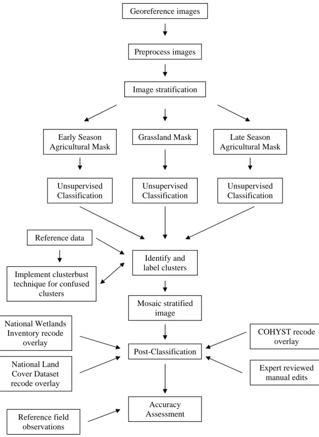
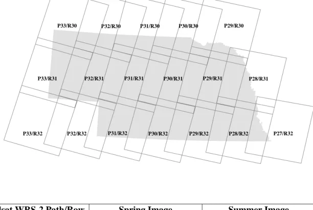
A total of 18 scenes are needed to cover the state of Nebraska. A multi-date classification technique was developed to generate the land cover map, then ancillary datasets were used to improve the discrimination among land cover types (Figure 2.1).
Land Cover Map Development
Overview
Nebraska GAP developed the land cover map using a multi-date classification approach, which captured differences in plant phenology of grasslands and identification of croplands (Figure 2.1). Early spring and late summer dates were selected within the same year, when possible (Figure 2.2). If a suitable scene was not available from the same year, a scene was selected from another year within our image catalog archive. The image archive received from EROS was preprocessed but each selected image was reviewed for accuracy and corrections were made as necessary.
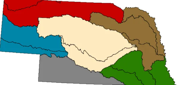
The State was divided into 6 geographic categories based upon similar ecological watersheds to reduce image size and processing time and to constrain land cover class assignment possibilities. Each multi-date path/row combination was subset to the watershed boundaries and the
Normalized Difference Vegetation Index (NDVI) was calculated to determine an agricultural and grassland mask to further segment the image. An unsupervised clustering algorithm was used to cluster each masked image and then assigned a land cover class. After class assignment, a mosaic of the State was created and ancillary data were used to further refine the classification. Images used for land cover classification were processed with ERDAS Imagine software.
Methodology
Preprocessing
Each selected Landsat 5 TM image was reviewed for accuracy and corrections made when necessary then reprojected to the Universal Transverse Mercator projection. Each image was subset to the intersecting watershed boundary (with 20km buffer). The two dates of imagery for each path/row were then “stacked” to create a 10 band multi-date image comprised of bands 2-5 and 7. Areas of cloud cover, jet contrails, and climatic anomalies were subset from images when necessary. In these instances, the subset areas were classified separately using the scene without cloud cover and not subject to the following image stratification technique.
Figure 2.1 Flowchart of land cover classification technique. Georeference images Preprocess images Image stratification Early Season Agricultural Mask
Grassland Mask Late Season Agricultural Mask Unsupervised Classification Identify and label clusters Reference data Implement clusterbust technique for confused
clusters Mosaic stratified image Post-Classification Accuracy Assessment National Wetlands Inventory recode overlay National Land Cover Dataset recode overlay COHYST recode overlay Expert reviewed manual edits Unsupervised Classification Unsupervised Classification Reference field observations
P27/R32 P33/R32 P29/R30 P33/R30 P28/R31 P33/R31 P29/R32 P31/R32 P28/R32 P32/R32 P30/R32 P30/R30 P31/R30 P32/R30 P29/R31 P32/R31 P31/R31 P30/R31
Landsat WRS-2 Path/Row Spring Image Summer Image
27/32 X 08/21/92 28/32 04/04/91 08/26/91 29/32 04/16/93 08/19/92 30/32 04/04/92 07/28/93 31/32 04/27/92 07/14/91 32/32 X 09/09/92 33/32 X 08/15/92 28/31 04/04/91 08/26/91 29/31 04/16/93 08/19/92 30/31 04/04/92 07/28/93 31/31 04/27/92 07/14/91 32/31 05/20/92 09/09/92 33/31 05/11/92 08/15/92 29/30 04/16/93 08/19/92 30/30 04/04/92 07/28/93 31/30 04/27/92 07/14/91 32/30 05/20/92 08/06/91 33/30 05/11/92 08/15/92
Figure 2.3 – Watershed divisions used to reduce image size, processing time, and land cover class assignment possibilities.
Imagestratification
Prior to classification, the image was stratified with agricultural and grassland masks derived from a mathematical expression. Initial NDVI values were calculated for each date. The spring NDVI value was then subtracted from the summer NDVI value and output as a new image. The calculated values were recoded into three groups to create the masks. The agricultural masks are represented by values on either end of the numerical spectrum due to extreme differences in NDVI values due to agricultural practices. For example, crops harvested in late summer would have low NDVI values in the spring because of barren soil or minimal vegetative canopy and by late summer a dense, vigorous canopy would be developed increasing the NDVI values. Spring crops would have the opposite properties. By contrast grasslands have a smaller range of NDVI values due to year round canopy cover and lack of intensive cultivation practices to ensure vegetation health. These masks were then applied to the raw image to create three images for processing.
Image Classification
An ISODATA (Iterative Self-Organizing Data Analysis Technique) unsupervised classification method was performed on the 10-band dataset for each masked image. The grassland image was separated into 50 clusters and each cropland image was separated into 10 clusters. Initial clusters were labeled based upon spectral and spatial characteristics. Aerial photography and field data were also used to label clusters.
If a cluster could not be identified, it was further processed using a technique termed “cluster busting” (Jensen et al 1987). This procedure subsets the cluster in question and the imagery is resubmitted through the classification algorithm and output into 10 clusters. These are then labeled in the same manner as described above.
Once all clusters are labeled for each stratified image, they are recombined to create a single thematic image. Once all were images were classified, a statewide mosaic was created. Further Classification Techniques
Additional datasets were used to enhance to the Nebraska GAP land cover map (Table 2.2).
Table 2.2: Ancillary data sets used for land cover mapping in Nebraska.
Data set Source
Watershed Boundary Nebraska Department of Natural Resources (DNR) National Wetlands Boundary (NWI) U.S. Fish and Wildlife Service
National Land Cover Dataset (NLCD) U.S. Geological Survey - EROS Data Center Cooperative Hyrology Study (COHYST) CALMIT, COHYST
Omernik Ecoregions U.S. Department of Agricultrue - Forest Service
National Wetlands Inventory
The dataset was acquired from the Army Corps of Engineers as a statewide mosaic of all
available digital coverage for the State of Nebraska. Edits to the dataset included the removal of quadrangle boundaries, closing open polygons, and altering the placement of some polygon labels for projection transformation.
The NWI codes were used to aggregate similar wetland types into a more identifiable
classification scheme. Queries were run on the vector dataset to create five new classes: riparian woodland, riparian shrubland, emergent wetland, aquatic bed wetland, and open water. In the event two wetland types were coded for the same polygon, the polygon was recoded using a surface perspective from an aerial platform to determine class assignment. For example, if the NWI attribute had the class definition PFO/PEM (palustrine forest / palustrine emergent), it would be assigned to the riparian woodland class because the forested element would be the dominant feature from an aerial platform. The recoded vector classes were converted into 30-meter grids and incorporated into the land cover mosaic.
Cooperative Hydrology Study (COHYST)
COHYST is a multi-agency project intended to improve understanding of hydrological conditions in the Platte River. The project involves assemblage and creation of numerous geospatial data layers to be used in modeling water resources. A detailed and accurate map of land cover and land use were mapped using 1997 Landsat TM satellite imagery. Agricultural crop types were recoded to agricultural/fallow agricultural fields and incorporated into the Nebraska GAP land cover classification.
National Land Cover Dataset (NLCD)
Derived from the early to mid-1990s Landsat TM satellite data, the NLCD is a 21-class land cover classification scheme applied consistently over the United States. The urban land cover classes were incorporated into the GAP land cover classification.
Omernik Ecoregions
The dataset was used as a guide to identify where floristic transitions may occur. It was found to be particularly useful for initial identification of grasslands. Omernik’s ecoregion map was used
to create the western boundary of the Upland Tallgrass Prairie class due to spectral confusion of the Upland Tallgrass Prairie and Little Bluestem-Gramma Mixedgrass Prairie classes.
Nebraska Natural Resources Conservation Service (NRCS) Expert Review
County maps of the initial classification were sent to NRCS district conservationists for local expert review. Annotations detailing misclassification were made on the hard copy map by local experts and returned for interpretation. These remarks served as a surrogate to the land cover accuracy assessment. Most of the misclassifications identified by the field experts were agricultural fields due to increasing agricultural activity in Nebraska. Recoding these pixels to agricultural fields was done on a case-by-case basis.
To solicit expert assessment of the draft land cover map, the Nebraska Gap Analysis Project and the Nebraska State Office of the Natural Resources Conservation Service sent out relevant county-level maps to District Conservationist NRCS Offices. The District Conservationists coordinated review of the hard-copy maps utilizing staff from 81 NRCS Offices statewide. Local experts in reviewed the draft maps and identified misclassifications by annotating the hard-copy map with a series of general and specific comments.
Of the 93 county maps sent out, 75 were returned, yielding a response rate of over 80%. While 10 maps indicated no change, 65 were annotated with specific comments. General and specific comments were recorded from each map. Specific comments, defined as comments noting misclassification of particular groups of pixels, were then tabulated into a special confusion matrix reporting only misclassification errors; thus, all elements of the matrix were located off the principal diagonal (cf. tables in Henebry et al. 2000).
Misclassifications identified on the draft land cover map were then compared against a
subsequent version of the map that incorporated additional sources of information. A second special confusion matrix was generated to determine whether misclassifications had been corrected by incorporation of multiple data sources. Remaining misclassifications deemed significant were manually recoded. The decision to recode pixels into the “Agricultural Fields” class was made on a case-by-case basis. Adjustments were made by comparing the latest draft with the National Land Cover Data product, relevant DOQQs, and a map of Nebraska’s native vegetation. A third special confusion matrix was then generated.
The inclusion of additional data sources took care of 302 (31%) of the specific comments. Manual editing of the significant misclassifications took care of 241 (35%) remaining comments. The two-stage revision eliminated 543 (55%) of the specific comments made by the expert
reviewers. Of the remaining 446 misclassifications, 372 (83%) were identified by the reviewers as “Agricultural Fields”. The classes contributing to most of this remaining error were
“Barren/Sand/Outcrop” (144 or 39%) and “Lowland Tallgrass Prairie” (124 or 33%). The second most confused class was “Little Bluestem-Grama Mixedgrass Prairie” at 53 (12%) remaining comments. Two woodland classes contributed to most of the error remaining after revisions: “Deciduous Forest/Woodland” (26 or 49%) and “Evergreen Forest/Woodland” (21 or 40%).
Inclusion of additional data significantly improved the land cover map. Further revision by manual recoding yielded a reduction of misclassification by 55% from the original draft map.
Results
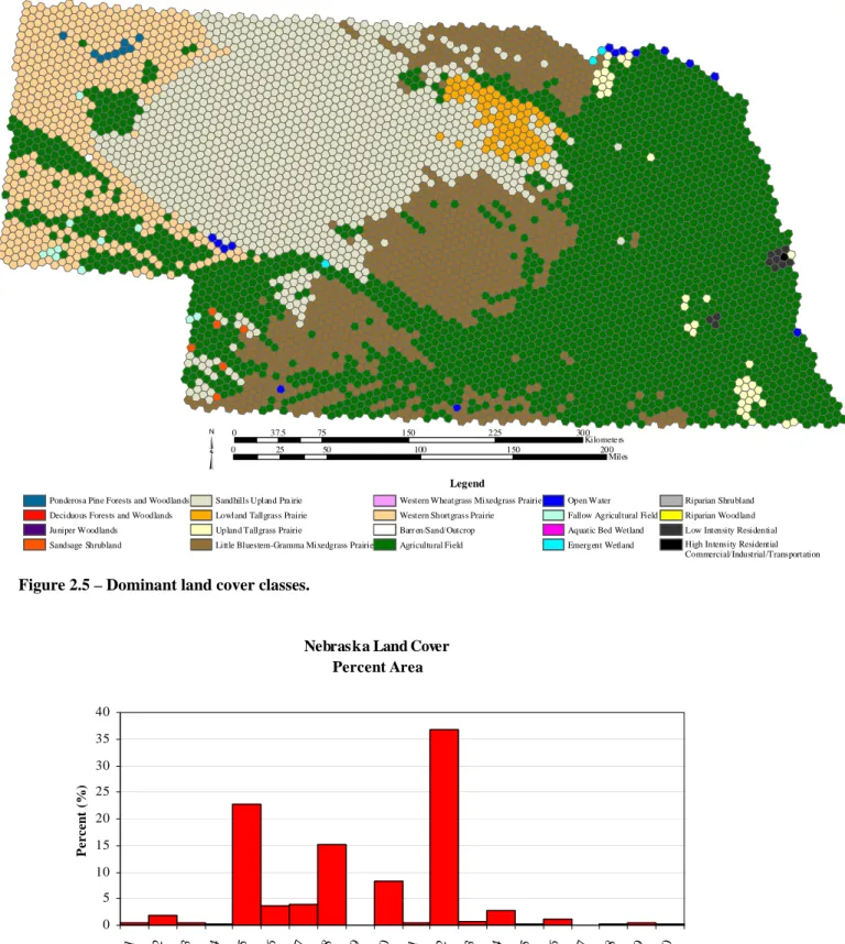
The final thematic map identifies 20 different land cover classes (Figure 2.4). Agricultural fields and grasslands (Figures 2.5 and 2.6) dominate the landscape of Nebraska. As Table 2.3 shows, almost 40% of the State is under cultivation. Much of the State’s agricultural fields are
maintained with irrigation systems. The most intensive use is found along the Platte River and south central Nebraska. The second most identifiable feature is the Sandhills Upland Prairie class (23%) found throughout the Nebraska Sandhills. The Sandhills are vegetated sand dunes making cultivation difficult. The Sandhills Upland Prairie class and the 6 other grassland classes account for 54% of the states land cover and are primarily managed for ranching purposes. Grazing and fire suppression have altered the native vegetation composition of these grasslands. Five woody vegetation classes were mapped for the State of Nebraska and cover 3% of the state. These classes are usually found along riparian corridors and canyons. Discrimination between forests and woodlands were not conducted because the scarcity of occurrence and linear pattern of distribution. Ponderosa Pine Forests and Woodlands are found along the Pine Ridge in northwest Nebraska and the Niobrara River. Of note, a man-made Ponderosa Pine Forest can be seen in the middle of the Sandhills. Deciduous Forests and Woodlands are largely found along rivers and streams. These stands have become more dense and extensive due to stream
channelization and flood control. Juniper woodlands (mainly cedar) are increasing across the state due to the suppression of wildfires. Juniper woodlands are concentrated in valleys,
canyons, and other protected lowlands and are usually mixed with deciduous woody vegetation. Although open water and wetland classes cover only 2% of the State, these features figure prominently into vertebrate species distribution. Of note, is the Platte River that cuts across the middle of the state and the various reservoirs found across the State. Wetlands fed by
groundwater are found in the Sandhills and are important for waterfowl breeding. Other wetlands are found in the Rainwater Basin of South Central Nebraska. These wetlands are fed by runoff and are utilized by birds and waterfowl during migration along the Central Corridor. Only the largest wetlands are filled year round.
0 25 50 100 150 200 Miles 0 37.5 75 150 225 300 Kilometers
³
LegendPonderosa Pine Forests and Woodlands Deciduous Forests and Woodlands
Sandhills Upland Prairie Lowland Tallgrass Prairie
Western Wheatgrass Mixedgrass Prairie Western Shortgrass Prairie
Open Water
Fallow Agricultural Field
Riparian Shrubland Riparian Woodland
Land Cover Classification of Nebraska
Figure 2.6 – Proportional distribution among land cover classes. Figure 2.5 – Dominant land cover classes.
0 37.5 75 150 225 300 Kilomete rs 0 25 50 100 150 200 Miles
³
LegendPonderosa Pine Forests and Woodlands Deciduous Forests and Woodlands Juniper Woodlands Sandsage Shrubland
Sandhills Upland Pra irie Lowland Tallgrass Prairie Upland Tallgrass Prairie
Little Bluestem-Gramma Mixedgrass Prairie
Western Wheatgrass Mixedgrass Prairie Western Shortgrass Prairie Barr en/Sand/Outcrop Agricultural Field
Open Water Fallow Agricultural Field Aquatic Bed Wetland Emergent Wetland
Riparian Shrubland Riparian Woodland Low Intensity Residential High Intensity Residential Commercial/Industrial/Transportation
Dominant Land Cover of Nebraska
Nebraska Land Cover Percent Area 0 5 10 15 20 25 30 35 40 1 2 3 4 5 6 7 8 9 10 11 12 13 14 15 16 17 18 19 20
Land C ove r C lass
P erce n t ( % )
Accuracy Assessment
Introduction: GAP land cover maps are primarily compiled to answer the fundamental question in gap analysis: what is the current distribution and management status of the nation's major natural land cover types and wildlife habitats? Besides giving a measure of overall reliability of the land cover map for Gap Analysis, the assessment also identifies which general classes or which regions of the map do not meet the accuracy objectives for the Gap Analysis Program. Thus the assessment identifies where additional effort will be required when the map is updated. We report the results of the accuracy assessment, believing that the map is the best map currently available for the project area.
The purpose of accuracy assessment is to allow a potential user to determine the map's "fitness for use" for their application. It is impossible for the original cartographer to anticipate all future
Land Cover
Value Land Cover Name km2 mile2 Acre Hectare Percent
1 Ponderosa Pine Forests and Woodlands 1070.61 413.36 264551.67 107060.67 0.53
2 Deciduous Forest/Woodland 3484.83 1345.50 861117.80 348483.33 1.74
3 Juniper Woodland 1022.11 394.64 252568.64 102211.29 0.51
4 Sandsage Shrubland 677.44 261.56 167398.85 67744.17 0.34
5 Sandhills Upland Prairie 45572.45 17595.62 11261155.26 4557245.13 22.74
6 Lowland Tallgrass Prairie 7301.69 2819.20 1804280.52 730169.19 3.64
7 Upland Tallgrass Prairie 7885.88 3044.75 1948635.58 788587.83 3.94
8 Little Bluestem-Gramma Mixedgrass Prairie 30324.11 11708.20 7493221.34 3032410.59 15.13
9 Western Wheatgrass Mixedgrass Prairie 207.59 80.15 51297.62 20759.49 0.10
10 Western Shortgrass Prairie 16752.67 6468.24 4139658.60 1675266.75 8.36
11 Barren/Sand/Outcrop 926.94 357.89 229051.36 92694.15 0.46
12 Agricultural Fields 73618.49 28424.25 18191454.91 7361848.53 36.74
13 Open Water 1296.87 500.72 320461.30 129686.58 0.65
14 Fallow Agricultural Fields 5299.77 2046.25 1309595.54 529976.52 2.64
15 Aquatic Bed Wetland 404.11 156.03 99856.69 40410.72 0.20
16 Emergent Wetland 2384.78 920.77 589289.61 238477.95 1.19
17 Riparian Shrubland 219.53 84.76 54247.90 21953.43 0.11
18 Riparian Woodland 357.56 138.05 88354.02 35755.74 0.18
19 Low Intensity Residential 877.54 338.82 216842.82 87753.51 0.44
20 Commercial/Industrial/Transportation 686.36 265.01 169602.78 68636.07 0.34
Total 200371.32 77363.79 49512642.82 20037131.64 100.00 Table 2.3 – Mapped land cover types, total area, and percent area of the state.
user to evaluate fitness for their unique purpose. This can be described as the degree to which the data quality characteristics collectively suit an intended application. The information reported includes details on the database's spatial, thematic, and temporal characteristics and their accuracy.
Assessment data are valuable for purposes beyond their immediate application to estimating accuracy of a land cover map. The reference data is therefore made available to other agencies and organizations for use in their own land cover characterization and map accuracy assessments (see Data Availability for access information). The data set will also serve as an important training data source for later updates.
Even though we have reached an endpoint in the mapping process where products are made available to others, the gap analysis process should be considered dynamic. We envision that maps will be refined and updated on a regular schedule. The assessment data will be used to refine GAP maps iteratively by identifying where the land cover map is inaccurate and where more effort is required to bring the maps up to accuracy standards. In addition, the field sampling may identify new classes that were not identified at all during the initial mapping process.
Methods:
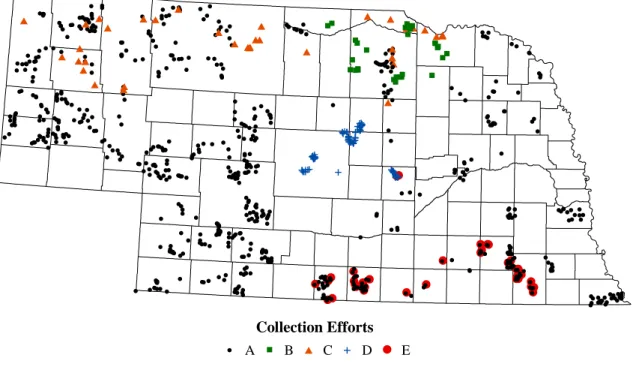
Our plans for land cover accuracy assessment were first linked to a multi-state EPA Region 7 land cover mapping project (cf. Nusser et al. 2001). Initial field data were collected in a pilot study during 1999 but, unfortunately, this project was not fully funded. This programmatic change necessitated some alternative strategies for conducting an accuracy assessment. During an initial phase of land cover mapping (1997-1998), teams were sent to sites across Nebraska to collect ground reference data that could be used in supervised classification. Since a later decision was made not to pursue a supervised classification, these “training” data were available to serve as potential ground referents for accuracy assessment. A total of 685 points were scouted. We refer to these data as Collection A. The final land cover classes had not yet been decided at the time these data were gathered. Once the classes were finalized, the field descriptions for these data were used to allocate each point to an appropriate land cover class. Following standard methods outlined in Congalton and Green (1999), an initial accuracy
assessment led to of an overall accuracy of less than 30%. Surprised by this result, we examined more closely the patterns of land cover occurrences in Collection A. The appearance of several odd patterns led us to conclude that the quality of Collection A was sufficiently suspect that it should be supplemented with other sources of reference data.
Four other collections of ground reference data were available for use in the accuracy
assessment. The data gathered in 1999 during the EPA pilot project was designated as Collection B. A project to map the land cover along the Niobrara River generated in 2002 ground reference data designated as Collection C. The tree cover in Loess Hills region in central Nebraska is complex with adjacent valleys being dominated either by deciduous or coniferous canopies. To facilitate cluster busting and labeling, we collected in 2001 ground reference data referred to as Collection D. In association with a NatureServe project, Dr. Kelly Kindscher (KU/Kansas Biological Survey) visited in 2002 a subset of the points in Collection A to evaluate the
accuracies of the GAP land cover map and Collection A. Dr. Kindscher’s field data are referred to as Collection E. Figure 2.7 illustrates the Collections’ geographic distribution.
Collection Efforts ! A " B # C E D ! E ! ! ! ! ! !!! ! ! ! !!!!!! ! ! !! !!! !! !! ! ! ! ! ! ! ! !!! !! ! ! ! ! !! ! ! ! ! !!! ! ! ! ! ! ! ! ! ! ! ! ! ! !! ! ! ! ! ! !! ! ! !! ! !! ! ! !!!! ! !! ! !!! ! ! ! ! ! ! ! ! ! ! ! ! ! ! ! ! ! ! ! ! ! !! !!! ! ! ! !! !! !!! ! ! !! !!!!! !! ! ! ! !! ! ! ! ! ! ! ! ! ! ! ! !! ! ! ! ! ! ! ! ! ! ! !! !!!! ! ! ! ! ! ! ! ! !! ! ! ! ! ! ! ! ! ! !! !! ! ! ! ! ! ! ! ! ! ! ! ! ! ! ! ! ! ! ! ! ! ! ! ! ! !! ! ! ! ! ! ! ! ! ! ! ! ! ! ! ! !!! !!! ! !! ! ! ! ! !! ! ! ! ! ! ! ! ! ! ! ! !! ! ! ! ! !!!!! ! ! ! ! ! !! !! ! ! ! ! ! ! ! ! ! ! ! ! ! ! ! ! !!!! ! ! ! ! ! !! !! ! ! ! ! ! ! !! ! ! ! ! ! ! !! !! ! !!! ! ! ! ! ! !!! ! ! ! ! ! ! !! ! !! ! ! ! ! ! !! ! !! ! ! ! !! !!!!!! ! ! !!! ! !!! ! ! ! ! ! ! ! ! ! ! ! ! ! ! !!!!!!! ! ! !!!!!! ! ! ! ! ! ! ! ! ! ! !!! ! !!!!! ! ! !! ! !! ! ! ! ! ! ! ! ! ! ! ! ! ! ! ! ! ! ! ! ! ! ! ! ! ! !! ! ! ! ! ! ! ! ! ! ! !!!! ! ! ! ! ! ! ! !!!!! ! ! ! ! ! ! ! ! ! ! ! ! ! !!!!!! !! ! ! ! ! ! ! ! ! !! ! !! ! !! ! !! ! ! !!!!! ! ! ! !!! ! ! ! ! ! ! !!!! !! ! ! !!!!! !!!! ! !!! !!! ! !! ! ! ! ! ! !! ! ! ! !!! !! ! ! ! ! ! ! !! ! ! ! !! !!!! ! ! !! !!!! !! ! ! ! !!! ! ! ! ! !! ! ! !!!! !! ! ! ! ! !! ! ! ! ! ! ! ! ! ! ! ! ! ! !!! ! !!!! !! # # # # # # # # # # # # # # # # # # # # # # # # # # # # # ! !! ! ! ! !!!! ! ! ! !! ! ! ! ! !!!! ! ! ! ! ! ! ! ! ! !! !! ! ! !! ! ! ! ! ! ! ! ! !! ! # # # # # # # # # EEEEEEEEEEEEEEEEEE E E E E EE E EEEEEEEEEEEEEEEEE E EEEEEEEEEEEEEEEEEEE EEEEEEEE E E E E E EEEEEEE E E E E EEE E "" " "" " " " "" " " " "" "" " " " "" "" " " " """ ""
Figure 2.7 Locations of sampling sites for field reference data used in accuracy assessment.
Results:
Table 2.4 provides the confusion matrix using Collection A. The overall accuracy is 29% with a significant Kappa value of 0.201. While the classification is far from random (Khat
z-score=12.74), there is considerable confusion between land cover classes, especially among the grassland types. Aggregating the cover classes into five broader categories leads to a significant increase in overall accuracy (61%; Table 2.5). These broader categories correspond to the landscape matrix within which organisms must find suitable habitat to persist. While the aggregation of the land cover classes into the broader categories is mostly straightforward, one category “Anthropolands” deserves some comment. Human influences on the landscape matrix and habitat availability can occur in many ways; however, the direct transformation of land to intensive human use is the most obvious. Anthropolands (from ανθρωπος, Greek for human) include the lands used for dense human settlement and commercial activity as well as active and fallow agricultural lands. Given the significant area in reservoirs, lakes, and farm ponds in Nebraska, it could be argued that the class 13 “open water” should be also be placed within the anthropolands category instead of the wetlands category. However, wildlife use of open water habitats is substantial and has more in common with wetlands than the lands intensively used by humans.
Challenging the aggregated classes with the field data from Collection B leads to an overall accuracy of 71% (Table 2.6). Overall accuracies are lower for Collections C (51%; Table 2.7), D (35%; Table 2.8), and E (38%; Table 2.9). Combining all of the field data into a confusion matrix on the aggregated classes leads to a higher overall accuracy of 60% (Table 2.10). A fundamental assumption of an accuracy assessment is that the reference data are correct. While this assumption may be only partially valid for any of the five Collections, it was possible to evaluate a non-random portion of Collection A by Collection E. Dr. Kindscher resurveyed 40 of the points from Collection A. In this sample only 13% (5/40) of the Collection A observations matched the GAP land cover classes. However, 41% (13/32) of the GAP land cover pixels corresponded to Kindscher’s observations and eight more observations had no comparable GAP class: brome (2) and CRP (6).
A simple accuracy assessment treats each class as having equivalent importance. A more refined approach is to weight the columns of the confusion matrix by abundance or prevalence of the class. The aggregated categories have the following area extents: Grasslands (53.9%),
Anthropolands (40.2%), Woodlands (3.0%), Wetlands (2.0%), and Shrublands (0.9%). (See Table 2.3 for the areal extents of the land cover classes.) Applying this approach to the
aggregated categories significantly increases the overall accuracy to 73% using all Collections (Table 2.11) and to 79% using Collection B alone (data not shown). Furthermore, application of the weighted approach to the complete set of land cover classes using Collection A yields an overall accuracy assessment of 47% (Table 2.12), a substantial increase over the results in Table 2.4.
Limitations and Discussion
A survey of the errors is instructive. As expected there is considerable confusion among
grassland cover types. Distinguishing among grassland types is very difficult because of smooth gradients of turnover in species composition between grassland communities. Differential phenologies in grassland species can help pick apart communities, but monitoring grassland phenology remains challenging at ground level, let alone from space (see Henebry 2003). The limited number of seasonal observations available in the Landsat TM imagery impaired
achieving a more robust discrimination between grassland types. A potential way to address this limitation in the future is to combine high temporal resolution data from coarser spatial
resolution synoptic sensors with the finer spatial resolution from the handful of nearly cloud-free Landsat scenes available for any particular area (Henebry et al. 2004; Viña et al. 2004).
Delineation of shrublands appears to be a weak spot in the land cover map. However, there were very few field reference samples among shrublands (28) and the aggregate category covered only 1824 km2 or 0.9% of the land area in Nebraska. Thus, it is difficult to judge whether the
shrublands are well-mapped. Clearly, this is a land cover type that needs more attention in any future mapping effort.
The dynamic nature of agriculture also poses significant problems for land cover mapping and assessment of accuracy. Field data were gathered in the late 1990’s and early 2000’s but the imagery is from the early 1990’s. Many of the misclassifications evident in the confusion matrix may arise from temporal decorrelation. Three phenomena will lead to problems: (1) expansion
and/or intensification of agriculture, e.g., starting to irrigate; (2) contraction or deintensification of agriculture, e.g., enrolling fields into CRP; and (3) big shifts in crop phenology, e.g., from maize to winter wheat. At an earlier stage of the mapping process, we found substantial effects from temporal decorrelation associated with agricultural land uses (Henebry et al. 2000). While some of these problems were addressed at that stage, the data were incomplete; thus, changes in agriculture land use and management practices affect multiple classes, not just class 12, as is evident from the spread of field observations along the rows and columns in Tables 2.4 and 2.12. Note that the weighted producer accuracy for class 12 is 90%, but the unweighted user accuracy is only 54%.
Accuracy assessment of land cover mapping involves multiple steps and multiple assumptions. The model of Nebraska land cover embedded in the choice of class labels reflects a perhaps optimistic expectation that all of these classes could be distinguished. Despite imperfect field reference data, the accuracy assessment of the final land cover map has shown that while things are generally correct at a coarser resolution, details are amiss. While accurate land cover
mapping is an important step, the primary aim of GAP is not the production of a land cover map; rather, the objective is to model wildlife habitat relationships and identify potential gaps in habitat. With this primary goal in mind and with an eye to the accuracy problems at the finer spatial scales, we decided to use the land cover map at a coarser spatial resolution while retaining the full distribution of the modeled land cover at a finer scale through the use of compositional arrays.
Table 2.4 – Accuracy assessment using ground reference data of Collection A
NaN = “Not a Number” results from division by zero (0).
Map
Field 1 2 3 4 5 6 7 8 9 10 11 12 13 14 15 16 17 18 19 20 row sum users' accuracy
1 6 2 4 2 1 15 0.40 2 1 18 7 7 6 21 29 1 1 1 92 0.20 3 2 5 7 7 1 16 4 42 0.17 4 2 3 1 6 5 1 1 1 1 21 0.10 5 47 4 4 3 1 1 1 1 62 0.76 6 10 16 19 2 13 2 20 5 1 4 1 93 0.21 7 2 3 2 2 7 4 10 30 0.07 8 1 1 1 54 1 2 30 39 1 13 4 1 148 0.20 9 15 4 19 24 1 10 1 74 0.00 10 1 4 2 1 8 0.25 11 2 2 2 6 0.00 12 3 1 1 6 5 12 21 16 93 11 3 1 173 0.54 13 1 1 2 4 0.00 14 0 NaN 15 0 NaN 16 1 5 6 1 5 1 2 1 2 6 30 0.20 17 1 1 0.00 18 0 NaN 19 2 1 1 5 2 11 0.46 20 1 1 0.00
column sum 9 40 17 4 172 44 25 152 0 100 4 182 12 19 4 14 1 1 5 6 811 accuracy overall
producer's
Table 2.5 – Accuracy assessment of aggregated classes using ground reference data of Collection A
Map
Field Woodlands Grasslands Shrublands Wetlands Anthropolands row sum users' accuracy
Woodlands (1-3+18) 47 66 2 5 29 149 0.32 Grasslands (5-10) 14 323 4 10 64 415 0.78 Shrublands (4+11+17) 0 20 2 1 5 28 0.07 Wetlands (13+15+16) 2 19 0 11 2 34 0.32 Anthropolands (12+14+19+20) 4 65 1 3 112 185 0.61
column sum 67 493 9 30 212 811 overall
producer's accuracy 0.70 0.66 0.22 0.37 0.53 0.61
Table 2.6 – Accuracy assessment of aggregated classes using ground reference data of Collection B
Map
Field Woodlands Grasslands Shrublands Wetlands Anthropolands row sum
users' accuracy Woodlands (1-3+18) 17 17 0 3 4 41 0.41 Grasslands (5-10) 8 167 12 2 13 202 0.83 Shrublands (4+11+17) 0 0 0 0 0 0 NaN Wetlands (13+15+16) 0 6 0 2 0 8 0.25 Anthropolands (12+14+19+20) 0 16 0 0 17 33 0.52
column sum 25 206 12 7 34 284 overall
producer's accuracy 0.68 0.81 0.00 0.29 0.50 0.71
Table 2.7 – Accuracy assessment of aggregated classes using ground reference data of Collection C
Map
Field Woodlands Grasslands Shrublands Wetlands Anthropolands row sum users' accuracy
Woodlands (1-3+18) 0 0 0 0 0 0 NaN Grasslands (5-10) 3 2 0 0 1 6 0.33 Shrublands (4+11+17) 0 0 0 0 0 0 NaN Wetlands (13+15+16) 0 5 0 5 0 10 0.50 Anthropolands (12+14+19+20) 1 8 0 0 12 21 0.57
column sum 4 15 0 5 13 37 Overall
producer's accuracy 0.00 0.13 NaN 1.00 0.92 0.51
Table 2.8 – Accuracy assessment of aggregated classes using ground reference data of Collection D
Map
Field Woodlands Grasslands Shrublands Wetlands Anthropolands row sum users' accuracy
Woodlands (1-3+18) 23 36 1 4 14 78 0.46 Grasslands (5-10) 1 2 0 0 0 3 0.67 Shrublands (4+11+17) 0 0 0 0 0 0 NaN Wetlands (13+15+16) 0 1 0 2 0 3 0.67 Anthropolands (12+14+19+20) 0 0 0 0 4 4 1.00
column sum 24 39 1 6 18 88 overall
producer's accuracy 0.96 0.05 0.00 0.33 0.22 0.35
Table 2.9 – Accuracy assessment of aggregated classes using ground reference data of Collection E
Map
Field Woodlands Grasslands Shrublands Wetlands Anthropolands row sum users' accuracy
Woodlands (1-3+18) 3 0 0 0 2 5 0.60 Grasslands (5-10) 3 7 0 1 2 13 0.54 Shrublands (4+11+17) 0 0 0 0 0 0 NaN Wetlands (13+15+16) 0 0 0 0 0 0 NaN Anthropolands (12+14+19+20) 0 15 0 0 4 19 0.21
column sum 6 22 0 1 8 37 overall
producer's accuracy 0.50 0.32 NaN 0.00 0.50 0.38
Table 2.10 – Accuracy assessment of aggregated classes using ground reference data from all Collections (A-E)
Map
Field Woodlands Grasslands Shrublands Wetlands Anthropolands row sum users' accuracy
Woodlands (1-3+18) 90 125 3 12 47 277 0.32 Grasslands (5-10) 23 500 16 12 93 644 0.78 Shrublands (4+11+17) 0 20 2 1 5 28 0.07 Wetlands (13+15+16) 3 33 0 21 3 60 0.35 Anthropolands (12+14+19+20) 7 91 1 3 149 251 0.59
column sum 123 769 22 49 297 1260 overall
producer's accuracy 0.73 0.65 0.09 0.43 0.50 0.60
Table 2.11 – Area-weighted accuracy assessment of aggregated classes using ground reference data from all Collections (A-E)
Map
Field %area Woodlands Grasslands Shrublands Wetlands Anthropolands row sum users' accuracy
Woodlands 2.9610 2.66589 3.702625 0.088863 0.355452 1.392187 8.205017 0.325
Grasslands 53.922 12.40208 269.6105 8.627536 6.470652 50.14755 347.2583 0.776
Shrublands 0.910 0 0.18206 0.018206 0.009103 0.045515 0.254884 0.071
Wetlands 2.039 0.061173 0.672903 0 0.428211 0.061173 1.22346 0.350
Anthropolands 40.166 2.811655 36.55152 0.401665 1.204995 59.84809 100.8179 0.594
column sum 100.000 17.9408 310.7196 9.13627 8.468413 111.4945 457.7596 overall
weighted producers'
Table 2.12 – Area-weighted accuracy assessment of classes using ground reference data from Collection A
NaN = “Not a Number” results from division by zero (0).
Map
Field % area 1 2 3 4 5 6 7 8 9 10 11 12 13 14 15 16 17 18 19 20 users' accuracy
1 0.53 3.21 1.07 2.14 1.07 0.53 0.40 2 1.74 1.74 31.3 12.2 12.2 10.4 36.5 50.4 1.74 1.74 1.74 0.20 3 0.51 1.02 2.55 3.57 3.57 0.51 8.16 2.04 0.17 4 0.34 0.68 1.01 0.34 2.03 1.69 0.34 0.34 0.34 0.34 0.10 5 22.7 1069 91.0 91.0 68.2 22.7 22.7 22.7 22.7 0.76 6 3.64 36.4 58.3 69.2 7.29 47.4 7.29 72.9 18.2 3.64 14.6 3.64 0.20 7 3.94 7.87 11.8 7.87 7.87 27.5 15.7 39.4 0.07 8 15.1 15.1 15.1 15.1 817. 15.1 30.3 454. 590. 15.1 197. 60.5 15.1 0.20 9 0.10 1.55 0.41 1.97 2.49 0.10 1.04 0.10 0.00 10 8.36 8.36 33.4 16.7 8.36 0.25 11 0.46 0.92 0.93 0.93 0.00 12 36.7 110. 36.7 36.7 220. 184. 441. 772. 588. 3417 404. 110. 36.7 0.54 13 0.65 0.65 0.65 1.29 0.00 14 2.64 NaN 15 0.20 NaN 16 1.19 1.19 5.95 7.14 1.19 5.95 1.19 2.38 1.19 2.38 7.14 0.20 17 0.11 0.11 0.00 18 0.18 NaN 19 0.44 0.88 0.44 0.42 2.19 0.88 0.45 20 0.34 0.34 0.00 weighted producer's accuracy 0.54 0.15 0.05 0.01 0.48 0.18 0.02 0.31 NaN 0.01 0.00 0.90 0.00 0.00 0.00 0.05 0.00 0.00 1.00 0.00 0.471